Resummed jet rates with heavy quarks in e⁺e^- collisions

Abstract

Expressions for Sudakov form factors for heavy quarks are presented. They are used to construct resummed jet rates in $e^{+}e^{-}$ annihilation. Predictions are given for production of bottom quarks at LEP and top quarks at the Linear Collider.

QCD@Work 2003 - International Workshop on QCD, Conversano, Italy, 14–18 June 2003

1 Introduction

The formation of jets is the most prominent feature of perturbative QCD in $e^{+}e^{-}$ annihilation into hadrons. Jets can be visualized as large portions of hadronic energy or, equivalently, as a set of hadrons confined to an angular region in the detector. In the past, this qualitative definition was replaced by quantitatively precise schemes to define and measure jets, such as the cone algorithms of the Weinberg–Sterman [1] type or clustering algorithms, e.g. the Jade [2, 3] or the Durham scheme ($k_{\perp}$ scheme) [4]. A refinement of the latter one is provided by the Cambridge algorithm [5]. Equipped with a precise jet definition the determination of jet production cross sections and their intrinsic properties is one of the traditional tools to investigate the structure of the strong interaction and to deduce its fundamental parameters. In the past decade, precision measurements, especially in $e^{+}e^{-}$ annihilation, have established both the gauge group structure underlying QCD and the running of its coupling constant $\alpha_{s}$ over a wide range of scales. In a similar way, also the quark masses should vary with the scale.

A typical strategy to determine the mass of, say, the bottom-quark at the centre-of-mass (c.m.) energy of the collider is to compare the ratio of three-jet production cross sections for heavy and light quarks [6, 7, 8, 9, 10]. At jet resolution scales below the mass of the quark, i.e. for gluons emitted by the quark with a relative transverse momentum $k_{\perp}$ smaller than the mass, the collinear divergences are regularized by the quark mass. In this region mass effects are enhanced by large logarithms $\ln(m_{b}/k_{\perp})$, increasing the significance of the measurement. Indeed, this leads to a multiscale problem since in this kinematical region also large logarithms $\ln(\sqrt{s}/k_{\perp})$ appear such that both logarithms need to be resummed simultaneously. A solution to a somewhat similar two-scale problem, namely for the average sub-jet multiplicities in two- and three-jet events in $e^{+}e^{-}$ annihilation was given in [11]. We report here on the resummation of such logarithms in the $k_{\perp}$-like jet algorithms [12] and provide some predictions for heavy quark production. A preliminary comparison with next-to-leading order calculations of the three-jet rate [6, 13, 14, 15] is presented.

2 Jet rates for heavy quarks

A clustering according to the relative transverse momenta has a number of properties that minimize the effect of hadronization corrections and allow an exponentiation of leading (LL) and next-to-leading logarithms (NLL) [4] stemming from soft and collinear emission of secondary partons. Jet rates in $k_{\perp}$ algorithms can be expressed, up to NLL accuracy, via integrated splitting functions and Sudakov form factors [4]. For a better description of the jet properties, however, the matching with fixed order calculations is mandatory. Such a matching procedure was first defined for event shapes in [16]. Later applications include the matching of fixed-order and resummed expressions for the four-jet rate in $e^{+}e^{-}$ annihilation into massless quarks [17, 18]. A similar scheme for the matching of tree-level matrix elements with resummed expressions in the framework of Monte Carlo event generators for $e^{+}e^{-}$ processes was suggested in [19] and extended to general collision types in [20].

We shall recall here the results obtained in [12] for heavy quark production in $e^{+}e^{-}$ annihilation. In the quasi-collinear limit [21, 22], the squared amplitude at tree-level fulfils a factorization formula, where the splitting functions $P_{ab}$ for the branching processes $a\to b+c$, with at least one of the partons being a heavy quark, are given by

$$P_{QQ}(z,q)\!\!\!\! = \!\!\!\!C_{F}\Bigg{[}\frac{1+z^{2}}{1-z}-\frac{2z(1-z)m^{2}}{q^{2}+(1-z)^{2}m^{2}}\Bigg{]}~{},$$

$$P_{gQ}(z,q)\!\!\!\! = \!\!\!\!T_{R}\left[1-2z(1-z)+\frac{2z(1-z)m^{2}}{q^{2}+m^{2}}\right]~{},$$ (1)

where $z$ is the usual energy fraction of the branching, and $q^{2}$ is the space-like transverse momentum. As expected, these splitting functions match the massless splitting functions in the limit $m\to 0$ for $q^{2}$ fixed. The splitting function

$$P_{gg}(z) = C_{A}\left[\frac{z}{1-z}+\frac{1-z}{z}+z(1-z)\right]~{}.$$ (2)

obviously does not get mass corrections at the lowest order.

Branching probabilities are defined through [12]

$$\!\!\!\!\!\!\!\!\!\!\!\!\Gamma_{Q}(Q,q,m)=\int\limits_{q/Q}^{1-q/Q}dz\frac{q^{2}}{q^{2}+(1-z)^{2}m^{2}}\,P_{QQ}(z,q)$$

$$\quad=\Gamma_{Q}(Q,q,m=0)+C_{F}\Bigg{[}\frac{1}{2}-\frac{q}{m}\arctan\left(\frac{m}{q}\right)$$

$$\quad-\frac{2m^{2}-q^{2}}{2m^{2}}\ln\left(\frac{m^{2}+q^{2}}{q^{2}}\right)\Bigg{]}~{},$$

$$\!\!\!\!\!\!\!\!\!\!\!\!\Gamma_{f}(Q,q,m)=\int\limits_{q/Q}^{1-q/Q}dz\frac{q^{2}}{q^{2}+m^{2}}\,P_{gQ}(z,q)$$

$$\quad=T_{R}\,\frac{q^{2}}{q^{2}+m^{2}}\,\left[1-\frac{1}{3}\frac{q^{2}}{q^{2}+m^{2}}\right]~{},$$

$$\!\!\!\!\!\!\!\!\!\!\!\!\Gamma_{g}(Q,q)=\int\limits_{q/Q}^{1-q/Q}dz\,P_{gg}(z)=2C_{A}\left(\ln\frac{Q}{q}-\frac{11}{12}\right)~{},$$ (3)

with

$$\Gamma_{Q}(Q,q,m=0) = 2C_{F}\left(\ln\frac{Q}{q}-\frac{3}{4}\right)~{},$$ (4)

and the Sudakov form factors, which yield the probability for a parton experiencing no emission of a secondary parton between transverse momentum scales $Q$ down to $Q_{0}$, read

$$\!\!\!\!\!\!\!\!\!\!\!\!\Delta_{Q}(Q,Q_{0})=\exp\Bigg{[}-\int\limits_{Q_{0}}^{Q}\frac{dq}{q}\frac{\alpha_{s}(q)}{\pi}\Gamma_{Q}(Q,q)\Bigg{]}\,,$$

$$\!\!\!\!\!\!\!\!\!\!\!\!\Delta_{g}(Q,Q_{0})=$$

$$\qquad\exp\Bigg{[}-\int\limits_{Q_{0}}^{Q}\frac{dq}{q}\frac{\alpha_{s}(q)}{\pi}\left(\Gamma_{g}(Q,q)+\Gamma_{f}(Q,q)\right)\Bigg{]}\,,$$

$$\!\!\!\!\!\!\!\!\!\!\!\!\Delta_{f}(Q,Q_{0})=\left[\Delta_{Q}(Q,Q_{0})\right]^{2}/\Delta_{g}(Q,Q_{0})\,,$$ (5)

where $\Gamma_{f}(Q,q)$ accounts for the number $n_{f}^{(l,h)}$ of active light or heavy quarks. Jet rates in the $k_{\perp}$ schemes can be expressed by the former branching probabilities and Sudakov form factors. For the two-, three- and four-jet rates

$${\cal R}_{2} = \left[\Delta_{Q}(Q,Q_{0})\right]^{2}\,,$$

$${\cal R}_{3} = 2\left[\Delta_{Q}(Q,Q_{0})\right]^{2}\,$$

$$\times \int\limits_{Q_{0}}^{Q}\frac{dq}{q}\frac{\alpha_{s}(q)}{\pi}\Gamma_{Q}(Q,q)\Delta_{g}(q,Q_{0})\,,$$

$${\cal R}_{4} = 2\left[\Delta_{Q}(Q,Q_{0})\right]^{2}\,$$ (6)

$$\times \Bigg{\{}\Bigg{[}\int\limits_{Q_{0}}^{Q}\frac{dq}{q}\frac{\alpha_{s}(q)}{\pi}\Gamma_{Q}(Q,q)\Delta_{g}(q,Q_{0})\Bigg{]}^{2}$$

$$+ \int\limits_{Q_{0}}^{Q}\frac{dq}{q}\Bigg{[}\frac{\alpha_{s}(q)}{\pi}\Gamma_{Q}(Q,q)\Delta_{g}(q,Q_{0})$$

$$\times\int\limits_{Q_{0}}^{q}\frac{dq^{\prime}}{q^{\prime}}\frac{\alpha_{s}(q^{\prime})}{\pi}\Gamma_{g}(q,q^{\prime})\Delta_{g}(q^{\prime},Q_{0})\Bigg{]}$$

$$+ \int\limits_{Q_{0}}^{Q}\frac{dq}{q}\Bigg{[}\frac{\alpha_{s}(q)}{\pi}\Gamma_{Q}(Q,q)\Delta_{g}(q,Q_{0})$$

$$\times\int\limits_{Q_{0}}^{q}\frac{dq^{\prime}}{q^{\prime}}\frac{\alpha_{s}(q^{\prime})}{\pi}\Gamma_{f}(q,q^{\prime})\Delta_{f}(q^{\prime},Q_{0})\Bigg{]}\Bigg{\}}\,,$$

where $Q$ is the c.m. energy of the colliding $e^{+}e^{-}$, and $Q_{0}^{2}=y_{\rm cut}Q^{2}$ plays the role of the jet resolution scale. Single-flavour jet rates in Eq. (2) are defined from the flavour of the primary vertex, i.e. events with gluon splitting into heavy quarks where the gluon has been emitted off primary light quarks are not included in the heavy jet rates but would be considered in the jet rates for light quarks.

In order to catch which kind of logarithmic corrections are resummed with these expressions it is illustrative to study the above formulae in the kinematical regime such that $Q\gg m\gg Q_{0}$. Expanding in powers of $\alpha_{s}$, jet rates can formally be expressed as

$${\cal R}_{n}=\delta_{n2}+\sum\limits_{k=n-2}^{\infty}\left(\frac{\alpha_{s}(Q)}{\pi}\right)^{k}\,\sum\limits_{l=0}^{2k}c^{(n)}_{kl},$$ (7)

where the coefficients $c^{(n)}_{kl}$ are polynomials of order $l$ in $L_{y}=\ln(1/y_{\rm cut})$ and $L_{m}=\ln(m^{2}/Q_{0}^{2})$. The coefficients for the first order in $\alpha_{s}$ are given by

$$c^{(2)}_{12}=-c^{(3)}_{12} = -\frac{1}{2}C_{F}(L_{y}^{2}-L_{m}^{2})\,,$$

$$c^{(2)}_{11}=-c^{(3)}_{11} = \frac{3}{2}C_{F}L_{y}+\frac{1}{2}C_{F}L_{m}\,.$$ (8)

For second order $\alpha_{s}$, with $n$ active flavours at the high scale, the LL and NLL coefficients read

$$c^{(2)}_{24} = \frac{1}{8}C_{F}^{2}\left(\vphantom{\frac{1}{2}}L_{y}^{2}-L_{m}^{2}\right)^{2}\,,$$

$$c^{(3)}_{24} = -\frac{1}{4}C_{F}^{2}\left(\vphantom{\frac{1}{2}}L_{y}^{2}-L_{m}^{2}\right)^{2}$$

$$- \frac{1}{48}C_{F}C_{A}\left(\vphantom{\frac{1}{2}}L_{y}^{4}-L_{m}^{4}\right)\,,$$

$$c^{(4)}_{24} = \frac{1}{8}C_{F}^{2}\left(\vphantom{\frac{1}{2}}L_{y}^{2}-L_{m}^{2}\right)^{2}$$

$$+ \frac{1}{48}C_{F}C_{A}\left(\vphantom{\frac{1}{2}}L_{y}^{4}-L_{m}^{4}\right)\,,$$

$$c^{(2)}_{23} = -C_{F}^{2}\left(\vphantom{\frac{1}{2}}L_{y}^{2}-L_{m}^{2}\right)\left(\frac{3}{4}L_{y}-\frac{1}{4}L_{m}\right)$$

$$- \frac{1}{3}\beta_{n}C_{F}\left(L_{y}^{3}-\frac{3}{2}L_{y}L_{m}^{2}+\frac{1}{2}L_{m}^{3}\right)$$

$$- \frac{1}{3}\left(\beta_{n}-\beta_{n-1}\right)C_{F}L_{m}^{3}\,,$$

$$c^{(3)}_{23} = \frac{1}{2}C_{F}^{2}\left(\vphantom{\frac{1}{2}}L_{y}^{2}-L_{m}^{2}\right)\left(3L_{y}-L_{m}\right)$$

$$+ \frac{1}{2}\beta_{n}C_{F}L_{y}\left(\vphantom{\frac{1}{2}}L_{y}^{2}-L_{m}^{2}\right)$$

$$+ \frac{1}{24}C_{F}C_{A}\left(\vphantom{\frac{1}{2}}3L_{y}^{3}-L_{m}^{3}\right)$$

$$+ \frac{1}{6}\left(\beta_{n}-\beta_{n-1}\right)C_{F}L_{m}\left(L_{y}^{2}-L_{y}L_{m}+2L_{m}^{2}\right)\,,$$

$$c^{(4)}_{23} = -C_{F}^{2}\left(\vphantom{\frac{1}{2}}L_{y}^{2}-L_{m}^{2}\right)\left(\frac{3}{4}L_{y}-\frac{1}{4}L_{m}\right)$$ (9)

$$- \frac{1}{6}\beta_{n}C_{F}\left(\vphantom{\frac{1}{2}}L_{y}^{3}-L_{m}^{3}\right)$$

$$- \frac{1}{8}C_{F}C_{A}\left(\vphantom{\frac{1}{2}}L_{y}^{3}-\frac{1}{3}L_{m}^{3}\right)$$

$$- \frac{1}{6}\left(\beta_{n}-\beta_{n-1}\right)C_{F}L_{y}L_{m}\left(L_{y}-L_{m}\right)\,.$$

Terms $\sim(\beta_{n}-\beta_{n-1})$ in the NLL coefficients, where the $\beta$-function $\beta_{n}$ for $n$ active quarks is given by

$$\beta_{n}=\frac{11\,C_{A}-2\,n}{12}~{},$$ (10)

are due to the combined effect of the gluon splitting into massive quarks and of the running of $\alpha_{s}$ below the threshold of the heavy quarks, with a corresponding change in the number of active flavours. With our definition of jet rates with primary quarks the jet rates add up to one at NLL accuracy. This statement is obviously realized in the result above order by order in $\alpha_{s}$.

The corresponding massless result [4] is obtained from Eqs. (8) and (9) by setting $L_{m}\to 0$. Notice that Eqs. (8) and (9) are valid only for $m\gg Q_{0}$ and therefore $m\to 0$ does not reproduce the correct limit, which has to be smooth as given by Eq.(2). Let us also mention that for $Q\gtrsim m$ there is a strong cancellation of leading logarithms and therefore subleading effects become more pronounced.

An approximate way of including mass effects in massless calculations, that is sometimes used, is the “dead cone” [23] approximation. The dead cone relies on the observation that, at leading logarithmic order, there is no radiation of soft and collinear gluons off heavy quarks. This effect can be easily understood from the splitting function $P_{QQ}$ in Eq. (1). For $q\ll(1-z)\ m$ this splitting function is not any more enhanced at $z\to 1$. This can be expressed via the modified integrated splitting function

$$\Gamma_{Q}^{\rm d.c.}(Q,q,m) = \Gamma_{Q}(Q,q,m=0)$$ (11)

$$+ 2C_{F}\ln\left(\frac{q}{m}\right)\Theta(m-q)\,.$$

To obtain this result the massless splitting function has been used, which is integrated with the additional constraint $z>1-q/m$. We also compare our results with this approximation.

3 Numerical results and comparison with fixed order calculations

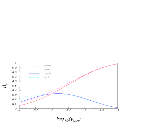
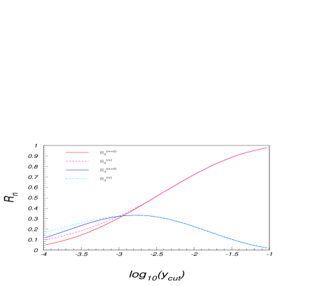
Figure 1: Effect of a $b$-mass of $5$ GeV on the single-flavour two- and three-jet rate at LEP1 energies as a function of the jet resolution parameter in the $k_{\perp}$ scheme. In the left plot this effect is treated through the full inclusion of masses into the splitting function, see Eq. (2), whereas in the plot on the right hand side this effect is modeled through the dead cone, see Eq. (11).

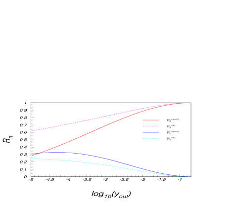
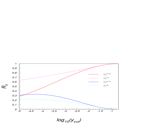
Figure 2: The effect of a $t$-mass of $175$ GeV on the single-flavour two- and three-jet rate as a function of the jet resolution parameter, at a potential Linear Collider operating at c.m. energies of 1 TeV. Again, in the left plot this effect is treated through the full inclusion of masses into the splitting function, see Eq. (2), whereas in the plot on the right hand side this effect is modeled through the dead cone, see Eq. (11).

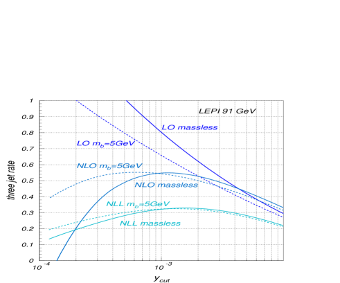
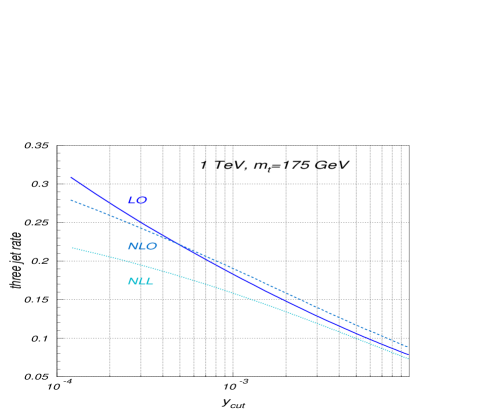
Figure 3: Comparison of LO, NLO and NLL predictions for the single-flavour three-jet rate as a function of the jet resolution parameter in the Cambridge algorithm for bottom quark production at LEP1 energies (left plot), and top quark production at a potential Linear Collider operating at c.m. energies of 1 TeV (right plot).

The impact of mass effects can be highlighted by two examples, namely by the effect of the bottom quark mass in $e^{+}e^{-}$ annihilation at the $Z$-pole, and by the effect of the top quark mass at a potential Linear Collider operating in the TeV region.

With $m_{b}=5$ GeV, $M_{Z}=91.2$ GeV, and $\alpha_{s}(M_{Z})=0.118$, the effect of the $b$-mass at the $Z$-pole on the two- and three-jet rates is depicted in Fig. 1 (left). The result obtained in the dead cone approximation is shown in Fig. 1 (right). Clearly, by using the full massive splitting function, the onset of mass effects in the jet rates is not abrupt as in the dead cone case and becomes visible much earlier. Already at the rather modest value of the jet resolution parameters of $y_{\rm cut}=0.004$, the two-jet rate, including mass effects, is enhanced by roughly $4\%$ with respect to the massless case, whereas the three-jet rate is decreased by roughly $3.5\%$. For even smaller jet resolution parameters, the two-jet rate experiences an increasing enhancement, whereas the massive three-jet rate starts being larger than the massless one at values of the jet resolution parameters of the order of $y_{\rm cut}\approx 0.001$. The curves have been obtained by numerical integration of Eq. (2). Furthermore, in order to obtain physical result the branching probabilities have been set to one whenever they exceed one or to zero whenever they become negative.

While in the case of bottom quarks at LEP1 energies the overall effect of the quark mass is at the few-per-cent level, this effect becomes tremendous for top quarks at the Linear Collider (Fig. 2).

In Fig. 3, leading order (LO) and next-to-leading order (NLO) predictions for three-jet rates are compared with the NLL result showed in the previous plots. Fixed order predictions for $b$-quark production clearly fail at very low values of $y_{\mathrm{cut}}$, by giving unphysical values for the jet rate, while the NLL predictions keep physical and reveal the correct shape. The latter is an indication of the necessity for performing such kind of resummations. Fixed order predictions work well for top production at the Linear Collider, a consequence of the strong cancellation of leading logarithmic corrections, and are fully compatible with our NLL result.

4 Conclusions

Sudakov form factors involving heavy quarks have been employed to estimate the size of mass effects in jet rates in $e^{+}e^{-}$ annihilation into hadrons. These effects are sizeable and therefore observable in the experimentally relevant region. A preliminary comparison with fixed order results have been presented, and showed good agreement. Matching between fixed-order calculations and resummed results is in progress [24].

References

• [1] G. Sterman and S. Weinberg, Phys. Rev. Lett.  39 (1977) 1436.
• [2] W. Bartel et al. [JADE Collaboration], Z. Phys. C 33 (1986) 23.
• [3] S. Bethke et al. [JADE Collaboration], Phys. Lett. B 213 (1988) 235.
• [4] S. Catani, Y. L. Dokshitzer, M. Olsson, G. Turnock and B. R. Webber, Phys. Lett. B 269 (1991) 432.
• [5] Y. L. Dokshitzer, G. D. Leder, S. Moretti and B. R. Webber, JHEP 9708 (1997) 001 [hep-ph/9707323].
• [6] G. Rodrigo, A. Santamaria and M. S. Bilenky, Phys. Rev. Lett.  79 (1997) 193 [hep-ph/9703358].
• [7] P. Abreu et al. [DELPHI Collaboration], Phys. Lett. B 418 (1998) 430.
• [8] A. Brandenburg, P. N. Burrows, D. Muller, N. Oishi and P. Uwer, Phys. Lett. B 468 (1999) 168 [hep-ph/9905495].
• [9] R. Barate et al. [ALEPH Collaboration], Eur. Phys. J. C 18 (2000) 1 [hep-ex/0008013].
• [10] G. Abbiendi et al. [OPAL Collaboration], Eur. Phys. J. C 21 (2001) 411 [hep-ex/0105046].
• [11] S. Catani, B. R. Webber, Y. L. Dokshitzer and F. Fiorani, Nucl. Phys. B 383 (1992) 419.
• [12] F. Krauss and G. Rodrigo, hep-ph/0303038; hep-ph/0309325.
• [13] G. Rodrigo, Nucl. Phys. Proc. Suppl.  54A (1997) 60 [hep-ph/9609213].
• [14] M. S. Bilenky, S. Cabrera, J. Fuster, S. Marti, G. Rodrigo and A. Santamaria, Phys. Rev. D 60 (1999) 114006 [hep-ph/9807489].
• [15] G. Rodrigo, M. S. Bilenky and A. Santamaria, Nucl. Phys. B 554 (1999) 257 [hep-ph/9905276]; Nucl. Phys. Proc. Suppl.  64 (1998) 380 [hep-ph/9709313].
• [16] S. Catani, L. Trentadue, G. Turnock and B. R. Webber, Nucl. Phys. B 407 (1993) 3.
• [17] L. J. Dixon and A. Signer, Phys. Rev. D 56 (1997) 4031 [hep-ph/9706285].
• [18] Z. Nagy and Z. Trocsanyi, Phys. Rev. D 59 (1999) 014020 [Erratum-ibid. D 62 (2000) 099902] [hep-ph/9806317].
• [19] S. Catani, F. Krauss, R. Kuhn and B. R. Webber, JHEP 0111 (2001) 063 [hep-ph/0109231].
• [20] F. Krauss, JHEP 0208 (2002) 015 [hep-ph/0205283].
• [21] S. Catani, S. Dittmaier and Z. Trocsanyi, Phys. Lett. B 500 (2001) 149 [hep-ph/0011222].
• [22] S. Catani, S. Dittmaier, M. H. Seymour and Z. Trocsanyi, Nucl. Phys. B 627 (2002) 189 [hep-ph/0201036].
• [23] Y. L. Dokshitzer, V. A. Khoze and S. I. Troian, J. Phys. G 17 (1991) 1602.
• [24] F. Krauss, G. Rodrigo, A. Schälicke and P. Tortosa, in preparation.