CERN-TH/2003-229
NEW PERSPECTIVES FOR B-PHYSICS FROM THE LATTICE

Abstract

We give an introduction to the problems faced on the way to a reliable lattice QCD computation of B-physics matrix elements. In particular various approaches for dealing with the large scale introduced by the heaviness of the b-quark are mentioned and promising recent achievements are described. We present perspectives for future developments.

1 B-physics and lattice QCD

The truly beautiful results from recent B-physics experiments [1, 2, 3, 4, 5] represented highlights of this conference. Some of them, such as the $\rm B-\bar{B}$ mass difference $\Delta m_{\rm d}$, require knowledge of QCD-matrix elements for their interpretation in terms of parameters of the standard model of particle physics and its possible extensions. This motivates investigations in lattice QCD, our best founded theoretical formulation of QCD. Indeed, this formulation allows for the computation of low energy hadronic properties through the Monte Carlo evaluation of the Euclidean path integral. While such a computation necessarily involves approximations, which we will discuss, the important property of the lattice approach is that all approximations can be systematically improved.

Before going into the details we summarize the goals of lattice QCD computations with b-quarks. They motivate the considerable effort involved.

• The determination of parameters of the CKM matrix, which in the Standard Model are fundamental parameters of Nature. In particular the unitarity triangle should be determined and over-constrained in order to test the Standard Model. The necessary non-perturbative matrix elements should be computed through lattice QCD.

• A precise computation of the b-quark mass, which enters many phenomenological predictions and plays a rôle in grand unification and other questions beyond the Standard Model.

• A determination of the spectrum and lifetimes of b-Hadrons.

• Non-perturbative tests of the Heavy Quark Effective Theory (HQET) which is applied frequently to simplify the dynamics of heavy quarks, but is difficult to test experimentally.

The starting point of a lattice computation is the QCD Lagrangian, formulated on the discretized 4-dimensional Euclidean space-time, i.e. on a hyper-cubic lattice with spacing $a$ [6, 7, 8]. The beauty of this theory is that it contains only the (bare) gauge coupling $g_{0}$ and the (bare) quark masses as parameters. After these parameters have been fixed by a small set of experimental observables, say the masses of proton, pion, kaon, D-meson and B-meson, all observables become predictions of the theory. In order to have a finite number of variables in the Monte Carlo evaluation of the path integral, one considers a finite space time of linear size $L$, mostly with periodic boundary conditions. One then has to approach

• the infinite volume limit, $L\to\infty$ and

• the continuum limit, $a\to 0$ .

While the statistical errors of the Monte Carlo decrease $\propto 1/\sqrt{\mbox{computer time}}$ at fixed $a$, $L$, a reduction of the total error requires to approach the above limits. Therefore the total error decreases much more slowly as computers get faster. Progress is made by better formulations of the problems, the development of better computational algorithms and the rapid increase in computer speed. Here we want to explain the particular challenges one faces in reaching small overall errors in B-Physics and discuss recent advances in facing them. Some results will be shown, mainly to illustrate the progress that has been made. A more comprehensive list of results can be found in [9, 10].

2 The challenges

2.1 Renormalization

One of the challenges that one faces has to do with the fact that interesting transitions originate from the electroweak interactions, which we can not treat simultaneously with QCD in the simulations. One then adopts the (good) approximation to treat the electroweak interactions at the lowest non-trivial order in the electromagnetic and weak coupling. Consequently one has an effective Hamiltonian, valid at energies far below the electroweak scale, which contains the quark and gluon fields but not the photon and the electroweak bosons. For example a left-left 4-fermion operator is one of the operators in the effective Hamiltonian and its matrix element determines $\Delta m_{\rm d}$. The renormalization of such operators is a non-trivial task, but besides perturbation theory [11] powerful non-perturbative approaches have been developed [12, 13, 14, 15] and they are continuously improved and applied to new operators [16]. We will come back to this challenge in our discussion of the HQET.

2.2 The multi-scale problem

Even after eliminating the electroweak scale by considering low energy matrix elements, b-physics always contains two more scales apart from the typical QCD scale $\Lambda={\rm O}(1{\rm GeV})$. The first is the scale of the light quark masses, or better the mass of the pion and the second is the large mass of the b-quark itself. To understand what this means in practical terms, consider a lattice with $32^{3}\times 64$ points, as it is presently possible in the quenched approximation but still prohibitively expensive for the full theory. Choosing $L\approx 2.5\,{\rm fm}$ and $a\approx 0.1\,{\rm fm}$, one notices that $L$ is comparable to the Compton wave length $m_{\pi}^{-1}$, namely $L\approx 2/m_{\pi}$, and at the same time the b-quark mass is larger than the inverse lattice spacing: $m_{{\rm b}}\approx\hbox{$3\over 2$}a^{-1}$. Instead we should have

$$L\gg m_{\pi}^{-1}\,,$$ (1)

$$a\ll m_{{\rm b}}^{-1}\,,$$ (2)

in order to keep finite size effects due to pion propagation around the periodic world small ( eq. (1)) and to properly resolve the propagation of a b-quark (eq. (2)). It is known that effects of the first type will become rapidly (exponentially) small when $L>4m_{\pi}^{-1}$ [17, 18], while the dominant discretization errors due to a heavy b-quark are given by ${\rm O}((am_{{\rm b}})^{2})$ if the theory is ${\rm O}(a)$-improved (i.e. linear $a$ effects are removed [19, 20]). The latter behavior sets in roughly for $a<\hbox{$1\over 4$}m_{{\rm b}}^{-1}$ [21]. On a $32^{3}\times 64$ lattice one is far from satisfying these constraints. An additional very relevant factor is that the computational cost of simulating full QCD grows rapidly when quark masses are lowered. This means that presently simulations at the physical values of the light quark masses are impossible.

In short: the light quarks are too light and the heavy quarks are too heavy for present computing capabilities.

In order to obtain results, a reformulation of the theory (or specific problem) is needed or extrapolations have to be performed.

2.3 Chiral extrapolations

Reliable extrapolations of numerical data are possible when sufficient analytic knowledge of the functional dependence on the extrapolation parameter exists and when the data are available in a range where the analytic formulae apply. Concerning the light quark mass dependence, chiral perturbation theory furnishes an expansion in terms of them, which is also applicable in the case of heavy-light mesons [22, 23]. Unfortunately it remains unclear up to now, how small the quark mass has to be in order that this expansion is applicable at the quantitative level. Most current simulations reach light quark masses which are about half as heavy as the strange quark mass and an agreement with the analytic formulae could not yet be established [24]. For recent reviews of the numerical situation with an emphasis on B-physics see refs. [25, 26].

As an example we would like to mention only that estimates of the uncertainty for the phenomenologically important ratio $\xi={(F_{\rm B_{\rm s}}\sqrt{B_{\rm B_{\rm s}}})/(F_{\rm B_{\rm d}}\sqrt{B_{\rm B_{\rm d}}})}$ range approximately from 5 % [27] to 10 % [28]. In our opinion these estimates have to be substantiated by simulations with smaller quark masses, where contact with the chiral perturbation theory expansion can be demonstrated. It appears that this requires both faster computers and the development of algorithms which perform better, in particular at small quark masses. First steps have been taken [29, 30, 31], and new ideas exist [32]. These very important developments are not specific to B-physics. We therefore do not discuss them further.

2.4 Heavy quarks on the lattice.

  

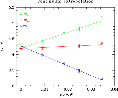
Figure 1: RGI charm mass from [33]. The length scale $r_{0}\approx 0.5\,{\rm fm}$ is derived from the force between static quarks.

Before coming to the methods for dealing with the problem of a heavy b-quark, let us give an illustration of the extent of the problem. It has been very well investigated for the charm quark [33, 34], which is a factor 4 lighter than the b-quark. In Fig. 1, we show the renormalization group invariant (RGI) charm mass, computed on four lattices, between $a=0.1\,{\rm fm}$ and $a=0.05\,{\rm fm}$. Three definitions of the renormalized quark mass were considered, differing by discretization errors ${\rm O}(a^{2})$. The figure shows that on lattices of the chosen size (from $16^{3}\times 32$ to $32^{3}\times 64$) one can control the discretization errors by extrapolation, but it is also obvious that this will not be possible for much heavier quarks. For b-quarks other approaches have to be considered. The following list summarizes what is being discussed.

• Extrapolation in the mass of the heavy quark, $m_{h}$.

• Effective theories which implement an expansion in $1/m_{{\rm b}}$: NRQCD[35] and HQET[36].

• The “Fermilab approach” [37].

• Anisotropic lattices with $a_{\rm time}\ll a_{\rm space}$ [38, 39].

• Combinations, in particular of 1. and 2.

• Extrapolation of finite volume effects in the quark mass [40, 41].

1. is clearly applicable once $m_{h}$ can be made large enough for the functional form, a power series in $1/m_{h}$, to be accurate. If $F(m_{h},am_{h})$ is the desired observable at finite lattice spacing and (unphysical) heavy quark mass, one has to evaluate

$$F(m_{{\rm b}},0)=\lim_{m_{h}\to m_{{\rm b}}}\lim_{am_{h}\to 0}F(m_{h},am_{h})$$ (3)

by two subsequent extrapolations whose order is important. In practice a residual uncertainty remains due to the assumptions made in the extrapolation $m_{h}\to m_{{\rm b}}$.
2. Effective theories should be rather accurate since $\Lambda/m_{{\rm b}}$ is a small expansion parameter, which controls both NRQCD and HQET. For reasons which will become clear below, NRQCD has predominantly been used in recent years although its continuum limit does not exist. In this theory one must keep the lattice spacing finite and control the discretization errors by adding terms to the Lagrangian that remove them approximately. An additional source of errors is that the coefficients in the Lagrangian are usually determined perturbatively. Below we will report on recent progress in HQET on the lattice.
3. The Fermilab approach was discussed at last year’s conference [26].
4. The possibility whether anisotropic lattices do permit a situation $a_{\rm space}m_{{\rm b}}>1$ for the interesting matrix elements is still under discussion [38, 39, 42]. In any case, giving up the symmetry between space and time allows for dimension four operators in the Lagrangian which break Euclidean invariance. To obtain a Euclidean invariant continuum limit (and thus Lorenz invariance after rotation to Minkowski space), these parameters have to be tuned properly. For full QCD with dynamical fermions, this is a non-trivial task if non-perturbative precision is desired.
5. Combining the effective theory at the lowest order, (the “static theory”), with (1.) turns extrapolations into an interpolations, reducing the influence of assumptions concerning the $1/m_{h}$-dependence considerably.
6. This new idea put forward at Tor-Vergata [40, 41] will be explained below.

The dominant approach in the last decade has been to compare several methods with their strengths and weaknesses and apply the result to phenomenology if different methods agree. New developments offer the chance to establish precise results without recourse to crosschecks through other methods.

3 New developments

3.1 Non-perturbative HQET

The lattice Lagrangian of (velocity zero) HQET,

$${\mathcal{L}}_{\rm{\rm HQET}}=\overline{\psi}_{\rm h}\,D_{0}\,\psi_{\rm h}-{c_{\rm kin}\over 2m_{{\rm b}}}\overline{\psi}_{\rm h}{\bf D}^{2}\psi_{\rm h}-{c_{\sigma}\over 2m_{{\rm b}}}\overline{\psi}_{\rm h}{\bf B}\cdot{\bf\sigma}\psi_{\rm h}+\ldots$$ (4)

has the same form as the continuum one to order $1/m_{{\rm b}}$; only the definitions of the covariant derivatives $D_{\mu}$ and the chromomagnetic field strength ${\bf B}$ are of course lattice specific. Together with a similar expansion of the operators who’s matrix elements one is interested in, it implements a systematic expansion in terms of $1/m_{{\rm b}}$ for B-mesons at rest [36]. Despite its attractive feature of having a continuum limit order by order in the $1/m_{{\rm b}}$-expansion, it has not been applied very much in recent years. The reason is threefold.

First, already in lowest order of the effective theory, called the static approximation, statistical errors grow rapidly as the Euclidean time-separation of correlation functions is made large (Fig. 2, filled symbols). But it is in the large time range, say $x_{0}>1.5\,{\rm fm}$, where masses and low energy matrix elements may safely be extracted.

Second, the number of parameters in the effective theory grows with the order in the expansion in $1/m_{{\rm b}}$.

Third, these parameters have to be determined non-perturbatively; otherwise the continuum limit does not exist [43] (fine tuning of parameters). This fact is due to the mixing of higher dimensional operators, such as ${1\over 2m_{{\rm b}}}\overline{\psi}_{\rm h}{\bf D}^{2}\psi_{\rm h}$ with lower dimensional ones, such as $\overline{\psi}_{\rm h}\,D_{0}\,\psi_{\rm h}$. A perturbative estimate of the parameters in the Lagrangian (or equivalently of the mixing coefficients) to order $g_{0}^{2l}$ would leave a perturbative

$${\rm remainder}\sim g_{0}^{2(l+1)}\,a^{-p}\;\sim\;a^{-p}\,[\ln(a\Lambda)]^{-(l+1)}\;\;\raisebox{-0.43057pt}{ $\stackrel{{\scriptstyle{a\to 0}}}{{\longrightarrow}}$}\;\;\;\infty\,.$$ (5)

This basic fact is unavoidable in an effective theory formulated with a cutoff.

Recently it was shown that the first point is overcome by considering alternative discretizations of the static theory [44], which differ only in the way the gauge fields enter the latticized covariant derivative. So-called HYP-links [45, 46] correspond to the triangles in Fig. 2 and result in errors at the % level at $x_{0}=1.5\,{\rm fm}$ with an only slow growth as $x_{0}$ is increased. Very importantly, it was also shown that $a$-effects with this new discretization are small [44, 47].

  

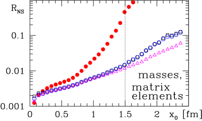
Figure 2: Noise to signal ratio of a B-meson correlation function in static approximation at $a\approx 0.08\,{\rm fm}$ [44]. The red bullets are for the original Eichten-Hill action while purple triangles correspond to the alternative discretization using HYP-links.

The second and third point above can be solved in one go if the parameters of HQET are non-perturbatively determined from those of QCD. In this way the predictive power of QCD is transfered to HQET.

The basic idea how to do this [48, 16], illustrated in Fig. 3, is easily explained. In a finite volume of linear extent $L_{0}={\rm O}(0.2\,{\rm fm})$, one may realize lattice resolutions such that $m_{{\rm b}}a\ll 1$ and the b-quark can be treated as a standard relativistic fermion. At the same time the energy scale $1/L_{0}={\rm O}(1\,{\rm GeV})$ is still significantly below $m_{{\rm b}}$ such that HQET applies quantitatively. Computing the same suitable observables in both theories relates the parameters of the HQET Lagrangian to those of QCD (matching). One then remains in HQET, changing iteratively to larger and larger volumes, and computes HQET observables in each step. Finally, in a physically large volume (linear extent ${\rm O}(2\,{\rm fm})$) the desired matrix elements are accessible. At the end any dependence on the unphysical intermediate volume physics is gone except for terms of the order ${\rm O}((L_{0}m_{{\rm b}})^{-(n+1)})$ if the effective theory was considered up to order $n$.

Figure 3: Connecting experimental observables to renormalized HQET. $\Gamma_{\rm stat}$ is a renormalized quantity in HQET and $\sigma_{\rm m}(\bar{g}^{2}(L))$ connects $\Gamma_{\rm stat}(L)$ and $\Gamma_{\rm stat}(2L)$. In the chosen example, the experimental observable is the mass of the B meson.

The strategy is formulated in such a way that the continuum limit can be taken in each individual step. To explain this we take a look at the simple equation which – at the lowest non-trivial order in $1/m_{{\rm b}}$ (static approximation) – relates the B-meson mass to the mass of the b-quark. For definiteness we take the RGI quark mass. It is given by the large $\mu$ asymptotics of the running mass, $\kern 1.0pt\overline{\kern-1.0ptm\kern-1.0pt}\kern 1.0pt(\mu)$ (in any scheme) via,

$$M_{\rm b}=\lim_{\mu\to\infty}\kern 1.0pt\overline{\kern-1.0ptm\kern-1.0pt}\kern 1.0pt_{\rm b}(\mu)\left[2b_{0}\bar{g}^{2}(\mu)\right]^{-d_{0}/2b_{0}}\,,$$ (6)

with $b_{0},d_{0}$ the lowest order coefficients of the beta-function and the anomalous dimension of the quark mass, respectively (conventions as in [15]). In contrast to $\kern 1.0pt\overline{\kern-1.0ptm\kern-1.0pt}\kern 1.0pt_{\rm b}(\mu)$, the RGI-mass, $M_{\rm b}$, is scheme independent.

In static approximation it is related to the mass of the B-meson, $m_{\rm B}$, via

$$m_{\rm B}=\underbrace{E_{\rm stat}-\Gamma_{\rm stat}(L_{2})}_{a\to 0\mbox{ in HQET}}+\underbrace{\Gamma_{\rm stat}(L_{2})-\Gamma_{\rm stat}(L_{0})}_{a\to 0\mbox{ in HQET}}+\underbrace{\Gamma(L_{0},{M_{\rm b}})}_{a\to 0\mbox{ in QCD}}+{\rm O}(\Lambda^{2}/M_{\rm b})\,.$$ (7)

Here $\Gamma(L,M_{\rm b})$ denotes the energy of a state with quantum numbers of a B-meson but defined in a finite volume world of linear extent $L$. The exact definition of this state [48] is not important to understand the idea but is quite relevant for the success of a numerical computation of $M_{\rm b}$. $\Gamma_{\rm stat}(L)$ is the same energy but evaluated in static approximation and $E_{\rm stat}$ denotes the energy (mass) of a B-meson state in large volume in static approximation. As mentioned before we have $L_{0}\approx 0.2{\rm fm}\,,\;L_{2}=4L_{0}$.

To appreciate eq. (7), one should first note that energies in the effective theory are related to energies in QCD by a shift $m_{\rm bare}$ which is universal in the sense of being independent of the state. This corresponds to a term $m_{\rm bare}\,\overline{\psi}_{\rm h}\,\psi_{\rm h}$ in eq. (4), which we have dropped there following standard conventions. Since the operator $\overline{\psi}_{\rm h}\,D_{0}\,\psi_{\rm h}$ mixes with the lower dimensional one $\overline{\psi}_{\rm h}\,\psi_{\rm h}$ under renormalization, the parameter $m_{\rm bare}$ is linearly divergent ($\sim 1/a$) and must be determined non-perturbatively. Its universality means

$$m_{\rm B} = E_{\rm stat}+m_{\rm bare}\,,$$ (8)

$$\Gamma(L,{M_{\rm b}}) = \Gamma_{\rm stat}(L)+m_{\rm bare}\,,$$ (9)

with one and the same $m_{\rm bare}$ at fixed $a$. One may now use eq. (9) to determine the parameter $m_{\rm bare}$ in the effective Lagrangian from QCD and then insert it into eq. (8) to determine $m_{\rm B}$. This represents the general logics for obtaining results in the HQET. In order to arrive at the continuum limit of the prediction, one groups terms as in eq. (7), where $m_{\rm bare}$ drops out of the energy differences $E_{\rm stat}-\Gamma_{\rm stat}(L_{2})$ and $\Gamma_{\rm stat}(L_{2})-\Gamma_{\rm stat}(L_{0})$ and the continuum limit can be taken separately for each of the terms as indicated.

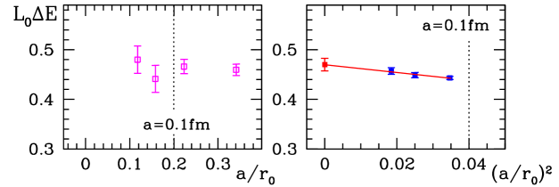
Figure 4: The combination $\Delta E=E_{\rm stat}-\Gamma_{\rm stat}(L_{2})$ as a function of the lattice spacing. Results with the new discretizations [44] (r.h.s) are compared with old results [49].

Indeed, in the quenched approximation a precise continuum limit has been taken for all terms [48] except for the energy difference $E_{\rm stat}-\Gamma_{\rm stat}(L_{2})$. Here [49] uses values for $E_{\rm stat}$ from the literature (l.h.s. Fig. 4). With the new discretization [44] more precise results are obtained (r.h.s. Fig. 4), and they also have the linear ${\rm O}(a)$-errors removed. The full analysis with the new data has not yet been performed. Using for the time being the value of $L_{0}(E_{\rm stat}-\Gamma_{\rm stat}(L_{2}))=0.46(5)$ one obtains [49] (we do not distinguish ${\rm O}(\Lambda/(L_{0}M_{\rm b}))$ and ${\rm O}(\Lambda^{2}/M_{\rm b})$ )

$$r_{0}M_{\rm b}=16.12(28)+{\rm O}(\Lambda^{2}/M_{\rm b})\;\to\;\kern 1.0pt\overline{\kern-1.0ptm\kern-1.0pt}\kern 1.0pt_{\rm b}^{\rm\overline{MS\kern-0.35002pt}\kern 0.35002pt}(\kern 1.0pt\overline{\kern-1.0ptm\kern-1.0pt}\kern 1.0pt_{\rm b}^{\rm\overline{MS\kern-0.35002pt}\kern 0.35002pt})=4.12(8){\rm GeV}+{\rm O}(\Lambda^{2}/M_{\rm b})$$ (10)

in the quenched approximation and with $r_{0}=0.5\,{\rm fm}$. It is worth emphasizing that such a result is based on the non-trivial relation between the bare quark masses on the lattice and the RGI-masses established in [15, 50].

3.2 Results for $F_{\rm B_{\rm s}}$

As a further new development, we show in Fig. 5 a recent computation of the decay constant of the $\rm B_{\rm s}$ meson in quenched approximation [51] using method number 5 in our list of Sect. 2.4. HQET predicts the mass dependence

$$F_{\rm PS}\sqrt{m_{\rm PS}}/C_{\rm PS}(M/\Lambda)=\Phi_{\rm RGI}+{\rm O}(1/m_{\rm PS})\,,$$ (11)

  

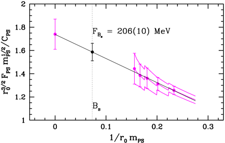
Figure 5: The continuum limit quenched pseudo scalar heavy-strange decay constant as a function of the inverse heavy-strange meson mass, $m_{\rm PS}$ [51].

of the decay constant $F_{\rm PS}$, where $\Phi_{\rm RGI}$ is independent of the heavy quark mass. It has recently been computed in the continuum limit of the static approximation [44]. The factor $C_{\rm PS}$ is a function of the ratio of the RGI mass of the heavy quark and the QCD Lambda parameter. It is now known quite accurately from perturbation theory due to the 3-loop result of [52]. Also the numbers of $F_{\rm PS}$ at finite quark mass shown in Fig. 5 have been extrapolated to the continuum limit [51, 34]. While the subsequent interpolation in $1/m_{\rm PS}$ is obviously safe, an extrapolation with just results for $1/(r_{0}m_{\rm PS})>0.15$ would depend on the functional form assumed. The present result $F_{\rm B_{\rm s}}=206(10)\,{\rm MeV}$ [51] is in good agreement with the recent one from the Tor-Vergata group [41].

3.3 The Tor-Vergata approach:
Extrapolation of finite volume effects in the quark mass

The starting point of this method is the same as in Sect. 3.1: in an intermediate volume (e.g. of size $L_{1}^{3}\times 2L_{1}$) the lattice spacing can be made small enough to be able to treat b-quarks as relativistic fermions. The decay constant $F(M_{h},L_{1})$ can then be computed for $M_{h}=M_{{\rm b}}$. While in the non-perturbative HQET, this was used to obtain the parameters in the effective theory, de Divitiis et al. remain in the relativistic theory, but introduce as their central observables finite size effects $\sigma_{\rm F}$ in the following way

$$F({M_{{\rm b}}},\infty)\approx F({M_{{\rm b}}},4L_{1})=\underbrace{F(M_{{\rm b}},4L_{1})\over F(M_{{\rm b}},2L_{1})}_{=\sigma_{\rm F}(M_{{\rm b}},2L_{1})}\times\underbrace{F(M_{{\rm b}},2L_{1})\over F(M_{{\rm b}},L_{1})}_{=\sigma_{\rm F}(M_{{\rm b}},L_{1})}\times F({M_{{\rm b}}},L_{1})\,.$$ (12)

The idea is that the finite size effects $\sigma_{\rm F}$ depend strongly on the dynamics of the light quark, but if $M_{h}$ is large enough, they hardly depend on that variable. It is thus expected that finite volume effects can smoothly be extrapolated in the heavy quark mass, $\sigma_{\rm F}(M_{{\rm b}},L_{1})=\lim_{M_{h}\to M_{{\rm b}}}\sigma_{\rm F}(M_{h},L_{1})$.

        

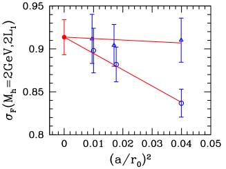
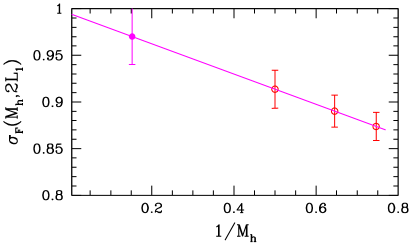
Figure 6: Quenched computation of $\sigma_{\rm F}(M_{{\rm b}},2L_{1})$ with the light quark mass equal to the strange quark mass.

Setting $L_{1}\approx 0.4\,{\rm fm}$, a numerical computation was performed in the quenched approximation. Of course, the three factors in eq. (12) are obtained by an extrapolation to the continuum limit at fixed $M_{h}$, followed by an extrapolation in $M_{h}$ to $M_{{\rm b}}$ for $\sigma_{\rm F}$, while $F({M_{{\rm b}}},L_{1})$ could be determined directly at $M_{h}=M_{{\rm b}}$. The most difficult extrapolations are those concerning the step $2L_{1}\to 4L_{1}$, since there $a\geq 4L_{1}/32\approx 0.05\,{\rm fm}$ on lattices with maximally $32^{3}\times 64$ points. They are shown in Fig. 6.

Comparing the r.h.s. of Fig. 6 with Fig. 5 one notices that (looking at the central values) in both cases the last point of the finite mass numbers differs from the result at $m_{\rm PS}=m_{\rm B_{\rm s}}$ by about 7%.

The final result is [41]

$$F_{\rm B_{\rm s}}=192(6)(4)\,{\rm MeV}\,.$$ (13)

Applying the same method also to the computation of the b-quark mass, yields [40] $\kern 1.0pt\overline{\kern-1.0ptm\kern-1.0pt}\kern 1.0pt_{\rm b}^{\rm\overline{MS\kern-0.35002pt}\kern 0.35002pt}(\kern 1.0pt\overline{\kern-1.0ptm\kern-1.0pt}\kern 1.0pt_{\rm b}^{\rm\overline{MS\kern-0.35002pt}\kern 0.35002pt})=4.33(10)\,{\rm GeV}$.

3.4 Summary

The new developments discussed in this section attack the problem of a heavy quark mass in ways where all necessary renormalizations are performed non-perturbatively (only in $C_{\rm PS}$ an ${\rm O}(\alpha(m_{{\rm b}})^{3})$ uncertainty remains) and the continuum limit can be taken in each step. They have been shown to be applicable in numerical computations, yielding good accuracy after propagating errors through all the steps. In fact, all the errors quoted in this section can be further reduced in the quenched approximation.

4 Perspectives

We start with some possible straight forward improvements of the above results.
First, the precision in Sect. 3.1 and 3.2 can easily be improved. Once this is done, one may quantify the size of $1/m_{{\rm b}}$ corrections rather precisely. In this context we note that it is surprising that so far there is no sign of $(1/m_{{\rm c}})^{2}$ terms in the charm region (see Fig. 5 and Fig. 6). Better precision is desirable to pin those down.
Second, a very promising improvement would be to combine the method of Sect. 3.3 with Sect. 3.1: the finite size effects $\sigma_{\rm F}$ can be computed in the HQET. Then the mass-extrapolation in Fig. 6 will also be turned into an interpolation and even larger precision and confidence can be achieved.

In our opinion it is most important (and more ambitious) to extend the calculations in the HQET to the level of including $1/m_{{\rm b}}$ corrections. We do not see any major obstacles on the way to reaching this goal. The severe problem of power divergences can be overcome by the non-perturbative matching of QCD and HQET sketched in Sect. 3.1. In contrast to the other methods discussed, the consequent use of an effective theory to describe the b-quark is a way to entirely eliminate the mass scale of the b-quark and thus the necessity of using large lattices. This then opens the possibility to obtain results in full QCD, once the usual (and large) problems with dynamical fermions, which have nothing to do with the heaviness of the b, are solved. Indeed, as emphasized in Sect. 2.3 we finally do need results with light dynamical quarks in order to apply them to phenomenology with confidence.
Acknowledgments. I am indebted to my collaborators in the ALPHA-collaboration for the possibility to present new results at this conference, prior to publication. I thank the Tor Vergata group for communications on their approach and for sending the data in Fig. 6. Furthermore I am grateful to the CERN theory division for its hospitality and L. Giusti for comments on the manuscript.

References

- [1] K. Abe, (2003), hep-ex/0308072.
- [2] Y. Pan, (2003), proceedings of “Physics in Collision 2003”.
- [3] S. Dasu, (2003), hep-ex/0309047.
- [4] Belle, B. Golob, (2003), hep-ex/0308060.
- [5] F. Azfar, (2003), hep-ex/0309005.
- [6] K.G. Wilson, Phys. Rev. D10 (1974) 2445.
- [7] M. Creutz, Cambridge, Uk: Univ. Pr. ( 1983) 169 P. ( Cambridge Monographs On Mathematical Physics).
- [8] I. Montvay and G. Münster, Cambridge, UK: Univ. Pr. (1994) 491 p. (Cambridge monographs on mathematical physics).
- [9] S.M. Ryan, Nucl. Phys. Proc. Suppl. 106 (2002) 86, hep-lat/0111010.
- [10] N. Yamada, (2002), hep-lat/0210035.
- [11] S. Capitani, Phys. Rept. 382 (2003) 113, hep-lat/0211036.
- [12] G. Martinelli et al., Nucl. Phys. B445 (1995) 81, hep-lat/9411010.
- [13] M. Lüscher, P. Weisz and U. Wolff, Nucl. Phys. B359 (1991) 221.
- [14] K. Jansen et al., Phys. Lett. B372 (1996) 275, hep-lat/9512009.
- [15] ALPHA, S. Capitani et al., Nucl. Phys. B544 (1999) 669, hep-lat/9810063.
- [16] R. Sommer, (2002), hep-lat/0209162.
- [17] M. Lüscher, Commun. Math. Phys. 104 (1986) 177.
- [18] J. Gasser and H. Leutwyler, Phys. Lett. 184B (1987) 83.
- [19] B. Sheikholeslami and R. Wohlert, Nucl. Phys. B259 (1985) 572.
- [20] M. Lüscher et al., Nucl. Phys. B478 (1996) 365, hep-lat/9605038.
- [21] ALPHA, M. Kurth and R. Sommer, (2001), hep-lat/0108018.
- [22] B. Grinstein et al., Nucl. Phys. B380 (1992) 369, hep-ph/9204207.
- [23] J.L. Goity, Phys. Rev. D46 (1992) 3929, hep-ph/9206230.
- [24] C. Bernard et al., (2002), hep-lat/0209086.
- [25] L. Lellouch, Nucl. Phys. Proc. Suppl. 117 (2003) 127, hep-ph/0211359.
- [26] A.S. Kronfeld, eConf C020620 (2002) FRBT05, hep-ph/0209231.
- [27] J.J. Sanz-Cillero, J.F. Donoghue and A. Ross, (2003), hep-ph/0305181.
- [28] A.S. Kronfeld and S.M. Ryan, Phys. Lett. B543 (2002) 59, hep-ph/0206058.
- [29] M. Hasenbusch, Phys. Lett. B519 (2001) 177, hep-lat/0107019.
- [30] M. Hasenbusch and K. Jansen, (2002), hep-lat/0211042.
- [31] M. Hasenbusch, plenary talk at “Lattice 2003”, Tsukuba , hep-lat/0310029.
- [32] M. Lüscher, JHEP 05 (2003) 052, hep-lat/0304007.
- [33] ALPHA, J. Rolf and S. Sint, JHEP 12 (2002) 007, hep-ph/0209255.
- [34] ALPHA, A. Jüttner and J. Rolf, Phys. Lett. B560 (2003) 59, hep-lat/0302016.
- [35] B.A. Thacker and G.P. Lepage, Phys. Rev. D43 (1991) 196.
- [36] E. Eichten and B. Hill, Phys. Lett. B234 (1990) 511.
- [37] A.X. El-Khadra, A.S. Kronfeld and P.B. Mackenzie, Phys. Rev. D55 (1997) 3933, hep-lat/9604004.
- [38] J. Harada et al., Phys. Rev. D66 (2002) 014509, hep-lat/0203025.
- [39] S. Hashimoto and M. Okamoto, Phys. Rev. D67 (2003) 114503, hep-lat/0302012.
- [40] G.M. de Divitiis et al., (2003), hep-lat/0305018v2.
- [41] G.M. de Divitiis et al., (2003), hep-lat/0307005.
- [42] S. Aoki, Y. Kuramashi and S.i. Tominaga, Prog. Theor. Phys. 109 (2003) 383, hep-lat/0107009.
- [43] L. Maiani, G. Martinelli and C.T. Sachrajda, Nucl. Phys. B368 (1992) 281.
- [44] ALPHA, M. Della Morte et al., (2003), hep-lat/0307021.
- [45] A. Hasenfratz and F. Knechtli, Phys. Rev. D64 (2001) 034504, hep-lat/0103029.
- [46] A. Hasenfratz, R. Hoffmann and F. Knechtli, Nucl. Phys. Proc. Suppl. 106 (2002) 418, hep-lat/0110168.
- [47] M. Della Morte et al., (2003), hep-lat/0309080.
- [48] ALPHA, J. Heitger and R. Sommer, Nucl. Phys. Proc. Suppl. 106 (2002) 358, hep-lat/0110016.
- [49] J. Heitger and R. Sommer, (October 2003), preprint DESY 03-156.
- [50] ALPHA, M. Guagnelli et al., Nucl. Phys. B595 (2001) 44, hep-lat/0009021.
- [51] J. Rolf et al., (2003), hep-lat/0309072.
- [52] K.G. Chetyrkin and A.G. Grozin, Nucl. Phys. B666 (2003) 289, hep-ph/0303113.