hep-ph/0309312
Atmospheric neutrinos: LMA oscillations, $U_{e3}$ induced interference and CP-violation

Abstract

We consider oscillations of the low energy (sub-GeV sample) atmospheric neutrinos in the three neutrino context. We present the semi-analytic study of the neutrino evolution and calculate characteristics of the $e$-like events (total number, energy spectra and zenith angle distributions) in the presence of oscillations. At low energies there are three different contributions to the number of events: the LMA contribution (from $\nu_{e}$-oscillations driven by the solar oscillation parameters), the $U_{e3}$-contribution proportional to $s_{13}^{2}$, and the $U_{e3}$ - induced interference of the two amplitudes driven by the solar oscillation parameters. The interference term is sensitive to the CP-violation phase. We describe in details properties of these contributions. We find that the LMA, the interference and $U_{e3}$ contributions can reach 5 - 6% , 2 - 3% and 1 - 2 % correspondingly. An existence of the significant ($>3-5\%$) excess of the $e$-like events in the sub-GeV sample and the absence of the excess in the multi-GeV range testifies for deviation of the 2-3 mixing from maximum. We consider a possibility to measure the deviation as well as the CP- violation phase in future atmospheric neutrino studies.

I Introduction

The existing results on atmospheric neutrinos SuperK are well described in terms of pure $\nu_{\mu}\leftrightarrow\nu_{\tau}$ oscillations with maximal or close to maximal mixing. Analysis of the Super-Kamiokande data gives SuperK ; sk-eps2003 mass squared difference and mixing in the interval:

$$\Delta m^{2}_{32}=(1.3-3.0)\times 10^{-3}{\rm eV}^{2}~{},~{}~{}~{}\sin^{2}2\theta_{23}>0.9,~{}~{}~{}~{}(90\%~{}{\rm C.L.}).$$ (1)

The results of SOUDAN SOUDAN and MACRO MACRO experiments are in a good agreement with (1). The oscillation interpretation (1) has been further confirmed by the results of the K2K experiment K2K .

Till now no compelling evidence of oscillations of the atmospheric $\nu_{e}$ has been obtained. The $3\nu$ global analysis of the atmospheric neutrino data is in agreement with no $\nu_{e}$-oscillations glob3 . The best fit point coincides with zero $\sin\theta_{13}$ within $1\sigma$ glob3 .

At the same time, after the first KamLAND result Kam we can definitely say that the $\nu_{e}$-oscillations of atmospheric neutrinos should appear at some level. Indeed, KamLAND has confirmed the large mixing MSW (LMA-MSW) solution of the solar neutrino problem. The combined analysis of the solar and KamLAND data leads to values of the oscillation parameters comb :

$$\Delta m^{2}_{21}=(5-10)\cdot 10^{-5}~{}{\rm eV}^{2}~{},~{}~{}\tan^{2}\theta_{12}=0.3-0.5~{}.$$ (2)

The parameters (2), which we will call the LMA parameters, should lead to oscillations of the $\nu_{e}$ component in the atmospheric neutrino flux.

The oscillations driven by the LMA parameters have been discussed before  yasuda ; thun ; Fogli ; kim ; sakai99 ; brunn ; orl1 ; Gonzalez-Garcia:2002mu . It was marked in Ref. Fogli that the effect of sub-leading oscillations driven by $\Delta m^{2}_{21}$ is significant only for the sub-GeV events and the size of effect is at the level of the statistical errors. In Ref. kim it was argued that the excess of e-like events in the sub-GeV sample favors the large mixing MSW solution of the solar neutrino problem.

The detailed study of the effect has been performed in our previous paper orl1 , where it was shown that the neutrino oscillations with LMA parameters can lead to an observable (up to 10 - 12 %) excess of the $e$-like events in the sub-GeV atmospheric neutrino sample. The excess has a weak zenith angle dependence in the low energy part of the sample and a strong zenith angle dependence in the high energy part. The excess rapidly decreases with energy of neutrinos, and it is strongly suppressed in the multi-GeV range. These signatures allow one to disentangle the effect of oscillations due to solar $\Delta m^{2}$ from other possible explanations of the excess.

It was shown that the relative excess is determined by the two neutrino transition probability $P_{2}$ and the “screening” factor:

$$\frac{F_{e}}{F_{e}^{0}}-1=P_{2}(r\cos^{2}\theta_{23}-1)~{},$$ (3)

where $F_{e}$ and $F_{e}^{0}$ are the electron neutrino fluxes with and without oscillations, $r$ is the ratio of the original muon and electron neutrino fluxes. The screening factor (in brackets) is related to existence of both the electron and muon neutrino in the original atmospheric neutrino flux. The appearance of excess (or deficiency) depends strongly on deviation of the $\nu_{\mu}-\nu_{\tau}$ (or 2 - 3) mixing responsible for the dominant mode of the atmospheric neutrino oscillations from maximal value. Indeed, in the sub-GeV region $r\approx 2$, so that the screening factor is very small when the $\nu_{\mu}-\nu_{\tau}$ mixing is maximal. Due to this factor the excess is in general small even though the $2\nu-$ probability can be of the order 1. The probability $P_{2}$, and consequently the excess, increase rapidly with $\Delta m^{2}_{21}$.

As far as the experimental results are concerned, there is a hint that some excess of the $e-$like events indeed exists in the sub-GeV range. Furthermore, the excess increases with decrease of energy within the sample super-data-used . In comparison with predictions based on the atmospheric neutrino flux from ref.honda the excess is about (12 - 15)% in the low energy part of the sub-GeV sample ($p<0.4$ GeV, where $p$ is the momentum of lepton). It has no significant zenith angle dependence. In the higher energy part of the sub-GeV sample ($p>0.4$ GeV) the excess is about 5% , and practically there is no excess in the multi-GeV region ($p>1.33$ GeV).

The excess is within estimated 20% uncertainty in the original atmospheric neutrino flux. The analysis of data with free overall normalization leads to the best fit $e-$like signal which practically excludes the excess super-data-used ; totsuka ; sk-eps2003 . However, the recent data on primary cosmic rays BESS ; AMS as well as new calculations of the atmospheric neutrino fluxes 3d-nufluxes change the situation. New results imply lower neutrino flux, and therefore larger excess which is difficult to explain by change of normalization super-data-used ; totsuka .

The $\nu_{e}$ oscillations can be also induced by non-zero 1-3 mixing and $\Delta m^{2}_{31}$ responsible for the dominant mode of the atmospheric neutrino oscillations yasuda ; threenu1 ; threenu2 ; threenu3 ; threenu4 ; four1 ; ADLS ; Bernabeu ; Gonzalez-Garcia:2002mu ; Gonzalez-Garcia:2003qf ; Maltoni:2003da . These oscillations require non-zero value of mixing matrix element $U_{e3}$. They are reduced to the vacuum oscillations for the sub-GeV sample. For the multi-GeV sample the Earth matter effect becomes important which can enhance the oscillations ADLS . For neutrinos which cross the core, the dominant effect is the parametric enhancement of oscillations. The size of effect is restricted by the CHOOZ bound on $U_{e3}$ CHOOZ .

In this paper we will further study the oscillation effects driven by the LMA oscillation parameters using an updated experimental information. We will consider an additional effect in the sub-GeV sample induced by non-zero 1-3 mixing. We study effects of the interplay of oscillations with the LMA parameters and non-zero $U_{e3}$. In particular, we will discuss the interference induced by non-zero $\sin\theta_{13}$. Some preliminary results of this study have been published in PS01 . The interference term depends on the CP-violation phase. We calculate effects of CP-violating phase and estimate a possibility to observe it in future atmospheric neutrino experiments.

The paper is organized as follows. In Sec. II we present the semi-analytical study of evolution of $3\nu$ system at low neutrino energies which correspond to the sub-GeV sample of events. We present the $3\nu$ neutrino transition probabilities in terms of the two neutrino probabilities. We calculate the latter numerically and study their properties. In Sec. II.C we give general expression for the flux of electron neutrinos. In Sec. III. we calculate the number of $e$-like events in the water Cherenkov detectors with and without oscillations. We consider the zenith angle and energy distributions of these events. We study separately effects of the LMA-oscillations (Sec. III.A), the $U_{e3}$ induced interference (Sec. III.B) and the CP-violation (Sec. III.C). In Sec. IV we discuss a possibility to measure the deviation of 2 - 3 mixing from maximum as well as the CP-violating phase in future atmospheric neutrino experiments. Discussion of the results and conclusions are given in sect. V.

II Evolution of the neutrino system

We consider the three-flavor neutrino system with hierarchical mass squared differences: $\Delta m^{2}_{21}=\Delta m^{2}_{\odot}<<\Delta m^{2}_{31}=\Delta m^{2}_{atm}$ (see Eqs. (1,2)). The evolution of the neutrino vector, $\nu_{f}\equiv(\nu_{e},\nu_{\mu},\nu_{\tau})^{T}$, is described by the equation

$$i\frac{d\nu_{f}}{dt}=\left(\frac{UM^{2}U^{\dagger}}{2E}+\hat{V}\right)\nu_{f},$$ (4)

where $E$ is the neutrino energy, $M^{2}\equiv diag(0,\Delta m_{21}^{2},\Delta m_{31}^{2})$ is the diagonal matrix of neutrino mass squared eigenvalues, $\hat{V}\equiv diag(V,0,0)$ is the matrix of matter-induced neutrino potentials with $V=\sqrt{2}G_{F}N_{e}$, $G_{F}$ and $N_{e}$ being the Fermi constant and the electron number density respectively. The mixing matrix $U$ is defined through $\nu_{f}=U\nu_{mass}$, where $\nu_{mass}\equiv(\nu_{1},\nu_{2},\nu_{3})^{T}$ is the vector of neutrino mass eigenstates. The matrix can be parameterized as

$$U=U_{23}D_{\delta_{CP}}U_{13}U_{12},~{}~{}~{}D_{\delta_{CP}}\equiv diag(1,1,e^{i\delta_{CP}}),$$ (5)

where $U_{ij}=U_{ij}(\theta_{ij})$ performs the rotation in the $ij$- plane on the angle $\theta_{ij}$. This parameterization coincides with the standard one up to (unphysical) renormalization of the mass eigenstates: $\nu_{mass}=D_{\delta_{CP}}^{*}\nu_{mass}^{\prime}$.

II.1 Propagation basis

The dynamics of oscillations is simplified in the “propagation” basis $\tilde{\nu}=(\tilde{\nu_{e}},\tilde{\nu}_{2},\tilde{\nu}_{3})^{T}$, which is related to the flavor basis by the unitary transformation

$$\nu_{f}=\tilde{U}\tilde{\nu},$$ (6)

and the matrix $\tilde{U}$ can be introduced in the following way. First, let us perform the rotation $\nu_{f}=U_{23}D_{\delta_{CP}}U_{13}\nu^{\prime}$. Using Eq. (4) we find that the instantaneous Hamiltonian for the new states $\nu^{\prime}$ takes the form

$$H^{\prime}=\frac{1}{2E}U_{12}M^{2}U^{\dagger}_{12}+U^{\dagger}_{13}VU_{13}~{},$$

or explicitly

$${H^{\prime}}=\left(\begin{array}[]{ccc}s_{12}^{2}\Delta m_{21}^{2}/2E+Vc_{13}^{2}&s_{12}c_{12}\Delta m_{21}^{2}/2E&Vs_{13}c_{13}\\ s_{12}c_{12}\Delta m_{21}^{2}/2E&c_{12}^{2}\Delta m_{21}^{2}/2E&0\\ V_{e}s_{13}c_{13}&0&\Delta m_{31}^{2}/2E+Vs_{13}^{2}\end{array}\right)\,,$$ (7)

($c_{12}\equiv\cos\theta_{12}$, $s_{12}\equiv\sin\theta_{12}$, etc.). Since the transformation $U_{23}D_{\delta_{CP}}U_{13}$ is constant (no dependence on density and therefore time), the evolution equation for $\nu^{\prime}$ is given by the Schrödinger equation with the Hamiltonian $H^{\prime}$. Notice that the CP-violation phase is removed from the equation for $\nu^{\prime}$, and it appears in the projection of the flavor basis on $\nu^{\prime}$ only. So, the evolution of system is CP-symmetric.

Second, let us make an additional $(\nu_{e}^{\prime}-\nu_{\tau}^{\prime})$ rotation, $\nu^{\prime}=U_{13}^{\prime}\tilde{\nu}$, which removes the off-diagonal terms $H_{13}^{\prime},H_{31}^{\prime}$ of the Hamiltonian (7). The angle of this rotation depends on the density:

$$\tan(\Delta\theta_{13})\approx s_{13}c_{13}\frac{2EV}{\Delta m^{2}_{13}}.$$ (8)

Since the low energy part of the sub-GeV sample is produced by neutrinos with energies (0.1 - 0.5) GeV the factor in Eq. (8) can be evaluated as

$$\frac{2EV_{e}}{\Delta m^{2}_{13}}=5.1\cdot 10^{-2}\frac{\rho Y_{e}}{g/cc}\cdot\frac{E}{1{\rm GeV}}\cdot\frac{3\cdot 10^{-3}{\rm eV}^{2}}{\Delta m^{2}}<0.1$$

for the matter density in the Earth $(3-10)$ g/cc. That is, the additional rotation is much smaller than the vacuum (1 - 3) rotation. The angle $\theta_{13}^{m}$ can be considered as a small correction to $\theta_{13}$:

$$\tilde{\theta}_{13}=\theta_{13}+\Delta\theta_{13}\approx\theta_{13}\left(1+\frac{2EV}{\Delta m^{2}_{31}}\right).$$ (9)

Basically, $\tilde{\theta}_{13}$ is the mixing angle in matter in the two neutrino approach: $\tilde{\theta}_{13}\approx\theta_{13}^{m}$, and plus sign in Eq. (9) reflects the fact that matter enhances the mixing in the neutrino channel for the normal mass hierarchy. In the antineutrino channel the sign is negative. For the inverted mass hierarchy the sign of $\Delta m^{2}_{31}$ should change, and the correction to $s_{13}$ (9) is positive in the antineutrino channel and negative in the neutrino channel.

As a consequence of the additional rotation we find the following.

1. The correction to $H_{11}^{\prime}$ element appears which can be considered as the correction to the potential:

$$\Delta H_{11}=\Delta V\approx-Vs_{13}^{2}\left(1-\frac{2EV}{\Delta m^{2}_{13}}\right).$$ (10)

It can be safely neglected.

2. The $H_{23}$ and $H_{32}$ elements are generated:

$$H_{23}=H_{32}=s_{12}c_{12}s_{13}V\left(\frac{\Delta m^{2}_{12}}{\Delta m^{2}_{13}}\right)$$ (11)

which are again negligible. Also corrections to the $H_{33}^{\prime}$ element can be neglected.

Combining the rotations introduced above we find the projection matrix $\tilde{U}$ (6) which defines the propagation basis:

$$\tilde{U}=U_{23}D_{\delta_{CP}}\tilde{U}_{13}=U_{23}D_{\delta_{CP}}U_{13}U_{13}^{\prime}=\left(\begin{array}[]{ccc}\tilde{c}_{13}&0&\tilde{s}_{13}\\ -\tilde{s}_{13}s_{23}e^{i\delta_{CP}}&c_{23}&\tilde{c}_{13}s_{23}e^{i\delta_{CP}}\\ -\tilde{s}_{13}c_{23}e^{i\delta_{CP}}&-s_{23}&\tilde{c}_{13}c_{23}e^{i\delta_{CP}}\end{array}\right)~{}.$$ (12)

In the propagation basis the evolution equation can be obtained from Eqs. (4, 12)

$$i\frac{d\tilde{\nu}}{dt}=\left(\tilde{H}+i\frac{d\tilde{\theta}_{13}}{dt}\hat{\lambda}\right)\tilde{\nu},$$ (13)

where

$$\tilde{H}\approx\left(\begin{array}[]{cc}H_{2}&0\\ 0&\Delta m_{31}^{2}/2E+Vs_{13}^{2}\end{array}\right)\,,$$ (14)

$$H_{2}=\frac{1}{2E}U_{12}M_{2}U_{12}^{\dagger}+Vc_{13}^{2},~{}~{}~{}~{}~{}M_{2}\equiv diag(0,\Delta m_{21}^{2}).$$ (15)

In (13) the matrix $\hat{\lambda}$ has all zero elements but $\lambda_{13}=-\lambda_{31}=1$. The last term in Eq. (13) can be evaluated as $d\tilde{\theta}_{13}/dt\sim\Delta\theta_{13}/R_{earth}$ for trajectories crossing the mantle only. For the core crossing trajectories the derivative can be large at the border between the core and the mantle. However, because of averaging of oscillations driven by $\Delta m_{31}^{2}$ we can neglect this dependence too.

According to Eq. (14), the state $\tilde{\nu}_{\tau}$ decouples from the rest of the system and evolves independently. The $(\tilde{\nu}_{e},\tilde{\nu}_{\mu})$ sub-system evolves according to the 2$\times$2 Hamiltonian $H_{2}$ ($\tilde{\nu}_{e}-\tilde{\nu}_{\mu}$ sub-matrix in Eq. (14)). This Hamiltonian is determined by the solar oscillation parameters $\Delta m_{21}^{2}$, $\tan^{2}\theta_{12}$ and the potential $V\approx Vc_{13}^{2}$. Thus, in the propagation basis the three neutrino problem is reduced to two neutrino problem.

Correspondingly, the evolution matrix S (the matrix of amplitudes) in the propagation basis $(\tilde{\nu}_{e},\tilde{\nu}_{\mu},\tilde{\nu}_{\tau})$ has the following form:

$$\tilde{S}\approx\left(\begin{array}[]{ccc}\tilde{A}_{ee}&\tilde{A}_{e\mu}&0\\ \tilde{A}_{\mu e}&\tilde{A}_{\mu\mu}&0\\ 0&0&\tilde{A}_{\tau\tau}\end{array}\right)~{}~{},~{}~{}$$ (16)

where

$$\tilde{A}_{\tau\tau}=\exp(-i\phi_{3})\,,\quad\quad\phi_{3}\approx\frac{\Delta m_{31}^{2}L}{2E},$$ (17)

and $L$ is the total distance traveled by neutrinos. Other amplitudes in (16), $\tilde{A}_{ee}$, $\tilde{A}_{e\mu}$,… should be found by solving the two neutrino evolution equation with the Hamiltonian $H_{2}$.

Since the oscillations driven by $\Delta m_{31}^{2}$ are averaged out, the dependence of the effects on the type of mass hierarchy (normal, inverted) appears only in the value of $\tilde{s}_{13}$ for neutrino and antineutrino channel. In what follows we will present results for normal mass hierarchy. For inverted hierarchy the difference of results is very small and can be largely absorbed in redefinition of $s_{13}$.

II.2 Flavor transitions

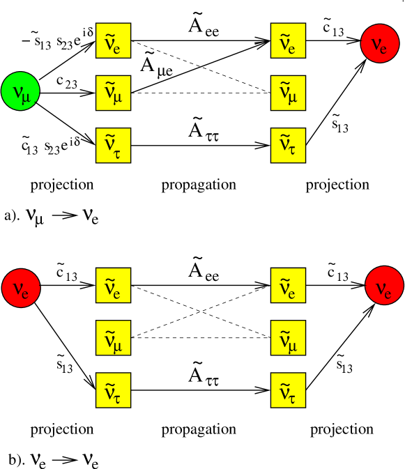
Figure 1: The neutrino transition scheme. Initial and final flavor states are shown in circles. In boxes we show the states of the propagation basis. Lines connect states between which the transitions can occur. The lines with arrows indicate transitions and projections relevant for oscillation channels of interest.

Let us find the probabilities of the $\nu_{\mu}\leftrightarrow\nu_{e}$ oscillations, $P_{\mu e}$, and the $\nu_{e}\leftrightarrow\nu_{e}$ oscillations, $P_{ee}$, relevant for our problem. The calculation proceeds in the three steps (see the transition scheme presented in fig. 1): (1) projection of the initial flavor state on to the propagation basis, (2) evolution in the propagation basis, (3) projection of the result of the evolution in the propagation basis on to the final flavor state. According to this picture the $S-$matrix in the flavor basis equals:

$$S=\tilde{U}\tilde{S}\tilde{U}^{\dagger},$$ (18)

where $\tilde{U}$ and $\tilde{S}$ are given by Eqs. (12) and (16).

Using Eqs. (18,16,12) we find

$$P_{\mu e}=\left|-\tilde{s}_{13}\tilde{c}_{13}s_{23}\tilde{A}_{ee}e^{i\delta_{CP}}+\tilde{c}_{13}c_{23}\tilde{A}_{\mu e}\right|^{2}+\tilde{s}_{13}^{2}\tilde{c}_{13}^{2}s_{23}^{2}.$$ (19)

For the sub-GeV sample the oscillations driven by $\Delta m_{31}^{2}$ are averaged out, so that there is no interference effect due to state $\tilde{\nu}_{\tau}$. At the same time, according to (19) the amplitudes $\tilde{A}_{ee}$ and $\tilde{A}_{\mu e}$ interfere. It is this interference which produces effect we interested in this paper. Notice that amplitudes $\tilde{A}_{ee}$ and $\tilde{A}_{\mu e}$ are both due to the solar oscillation parameters. However, their interference appears due to presence of the third neutrino (non-zero $s_{13}$). In the limit $s_{13}=0$ the interference disappears. In what follows we will call the interference of the amplitudes (with solar oscillation parameters) due to non-zero $U_{e3}\sim s_{13}$ as the $U_{e3}$ induced interference.

According to (19), there is no interference of the amplitudes driven by the atmospheric, $\Delta m_{31}^{2}$, and solar $\Delta m_{21}^{2}$ mass splittings. This interference is averaged out for the most part of the zenith angles. If $\cos\Theta_{\nu}>0$ (above the horizon), neutrinos propagate in the atmosphere, where the matter effect can be neglected. The effect of corresponding interference terms is very small: below (0.2 - 0.3) % (see Appendix), though we take it into account in our numerical calculations.

The probability (19) can be written explicitly as

$$P_{\mu e}=\tilde{c}_{13}^{2}c_{23}^{2}P_{2}-2\tilde{s}_{13}\tilde{c}_{13}^{2}s_{23}c_{23}(\cos\delta_{CP}R_{2}-\sin\delta_{CP}I_{2})+\tilde{s}_{13}^{2}\tilde{c}_{13}^{2}s_{23}^{2}(2-P_{2}),$$ (20)

where

$$P_{2}\equiv|\tilde{A}_{\mu e}|^{2}=1-|\tilde{A}_{ee}|^{2},~{}~{}~{}R_{2}\equiv Re(\tilde{A}_{\mu e}^{*}\tilde{A}_{ee}),~{}~{}~{}~{}I_{2}\equiv Im(\tilde{A}_{\mu e}^{*}\tilde{A}_{ee})$$ (21)

are the $2\nu$ probabilities in the propagation basis.

Similarly, we get $P_{ee}$:

$$P_{ee}=\tilde{c}_{13}^{4}(1-P_{2})+\tilde{s}_{13}^{4}.$$ (22)

No induced interference appears here due to zero projection of $\nu_{e}$ on to $\tilde{\nu}_{\mu}$ state (see (12)).

For antineutrinos, the probabilities $\bar{P}_{2}$, $\bar{R}_{2}$, $\bar{I}_{2}$ should be obtained by replacement of $V\rightarrow-V$ in the Hamiltonian $H_{2}$ of Eq. (14), and the sign of phase $\delta_{CP}$ should be changed:

$$\overline{P}_{2}=P_{2}(-V_{e}),~{}~{}~{}\overline{R}_{2}=R_{2}(-V_{e}),~{}~{}~{}\overline{I}_{2}=I_{2}(-V_{e}),~{}~{}~{}~{}~{}~{}~{}\overline{\tilde{s}}_{13}=\tilde{s}_{13}(-V_{e}),~{}~{}~{}\delta_{CP}\rightarrow-\delta_{CP}.$$ (23)

As a result,

$$\bar{P}_{\mu e}=\overline{\tilde{c}}_{13}^{2}c_{23}^{2}\bar{P}_{2}-2\overline{\tilde{s}}_{13}\overline{\tilde{c}}_{13}^{2}s_{23}c_{23}(\cos\delta_{CP}\bar{R}_{2}+\sin\delta_{CP}\bar{I}_{2}+\overline{\tilde{s}}_{13}^{2}\overline{\tilde{c}}_{13}^{2}s_{23}^{2}(2-\bar{P}_{2}),$$ (24)

$$\bar{P}_{ee}=\overline{\tilde{c}}_{13}^{4}(1-\bar{P}_{2})+\overline{\tilde{s}}_{13}^{4}.$$ (25)

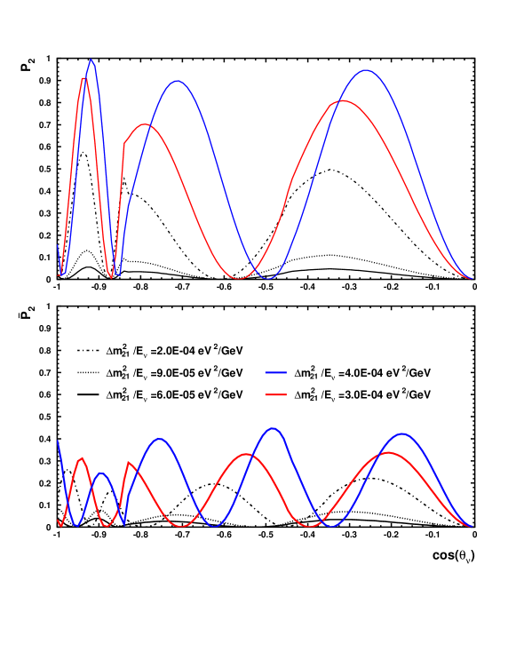
Figure 2: Zenith angle dependences of the transition probabilities for neutrinos, $P_{2}$, (upper panel), and for antineutrinos (lower panel), $\bar{P}_{2}$, for different values of $\Delta m^{2}_{12}/E$ and $\sin^{2}2\theta_{12}=0.82$.

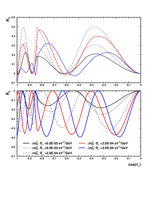
Figure 3: Zenith angle dependences of the real part of the interference probability for neutrinos, $R_{2}$ (upper panel), and for antineutrinos, $\bar{R}_{2}$ (lower panel), for different values of $\Delta m^{2}_{12}/E$ and $\sin^{2}2\theta_{12}=0.82$.

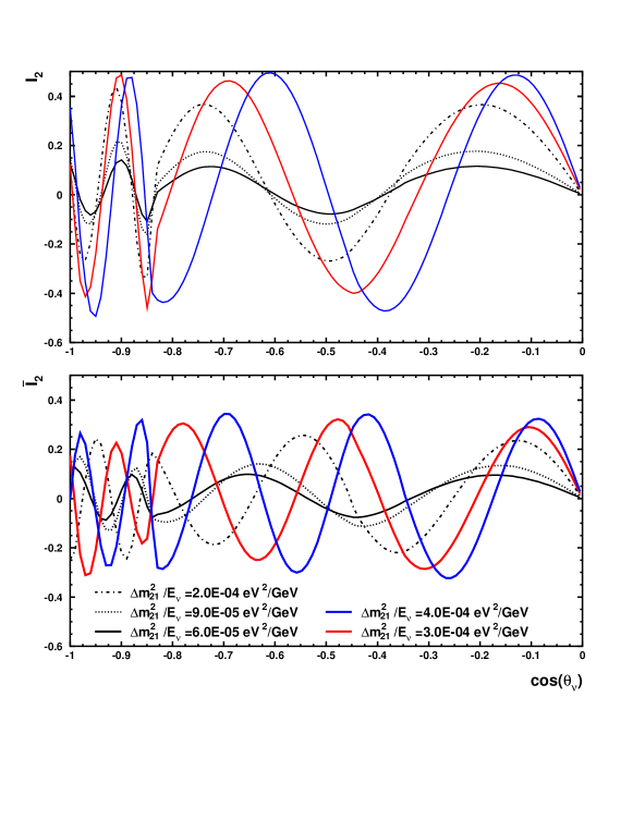
Figure 4: Zenith angle dependences of the imaginary part of the interference probability for neutrinos, $I_{2}$ (upper panel), and for antineutrinos, $\bar{I}_{2}$ (lower panel), for different values of $\Delta m^{2}_{12}/E$ and $\sin^{2}2\theta_{12}=0.82$.

Let us consider the two neutrino probabilities ${P}_{2}$, ${R}_{2}$, ${I}_{2}$ as well as $\bar{P}_{2}$, $\bar{R}_{2}$, $\bar{I}_{2}$ in details. We have calculated them numerically (see results in the figs. 2 - 4) using the distribution of density in the Earth from Ref. earthmodel .

Properties of the probabilities can be well understood using their expressions in medium with constant density:

$$P_{2}=\sin^{2}2\theta_{12}^{m}\sin^{2}\frac{\phi_{m}}{2}~{},$$ (26)

$$R_{2}=-\sin 2\theta_{12}^{m}\cos 2\theta_{12}^{m}\sin^{2}\frac{\phi_{m}}{2}~{},$$ (27)

$$I_{2}=-\frac{1}{2}\sin 2\theta_{12}^{m}\sin\phi_{m}.$$ (28)

Here $\phi_{m}=\Delta H_{12}R_{earth}\cos\Theta_{\nu}$, is the phase of oscillations in matter, where $\Delta H_{12}$ is the difference of the eigenvalues of the Hamiltonian in matter, $R_{earth}$ is the Earth radius and $\Theta_{\nu}$ is the zenith angle of neutrinos. In (26 - 28) $\theta_{12}^{m}$ is the 1-2 mixing in matter determined by

$$\sin 2\theta_{12}^{m}=\frac{\sin 2\theta_{12}}{\cos^{2}2\theta_{12}(1-E_{\nu}/E_{R})^{2}+\sin^{2}2\theta_{12}}.$$ (29)

The resonance neutrino energy equals

$$E_{R}\approx\frac{\Delta m^{2}_{21}\cos 2\theta_{12}}{2Vc^{2}_{13}}=0.238~{}{\rm GeV}\left(\frac{\Delta m^{2}_{21}}{7\cdot 10^{-5}{\rm eV}^{2}}\right)\left(\frac{2.0{\rm g/cm^{3}}}{Y_{e}\rho}\right)\cos 2\theta_{12}.$$ (30)

In the mantle, for the present best fit value $\Delta m^{2}_{21}=7.3\cdot 10^{-5}$ eV² and for $\sin^{2}2\theta_{12}=0.8$ we get $E_{R}~{}=~{}0.10$ GeV which is below the threshold of sub-GeV range. Therefore for $\Delta m^{2}_{21}\sim(5-7)\cdot 10^{-5}$ eV² and $E_{\nu}\sim(0.1-0.5)$ GeV the oscillations occur in the matter dominated regime when the potential is larger than the kinetic term: $V>\Delta m^{2}/2E$.

For $\Delta m^{2}_{21}/E_{\nu}<10^{-4}$ eV²/MeV the depth of oscillations is roughly proportional to $(\Delta m^{2})^{2}$. The oscillation length, $l_{m}$, is close to the refraction length, $l_{0}$, and only weakly depends on energy:

$$\sin^{2}2\theta_{m}\sim\sin^{2}2\theta_{12}\left(\frac{\Delta m^{2}_{21}}{2E_{\nu}V}\right)^{2}~{},~{}~{}~{}~{}~{}~{}l_{m}\approx l_{0}=\frac{2\pi}{V}.$$ (31)

With increase of $\Delta m^{2}/E$, the mixing parameter $\sin^{2}2\theta_{m}$, and consequently, $P_{2}$ approach 1 in the resonance in the neutrino channel. In the antineutrino channel the mixing and $\bar{P}_{2}$ increase but they are always below vacuum values.

The propagation (at least in the mantle of the Earth) has a character of oscillations with quasi constant depth and length. Correspondingly, $P_{2}$, $R_{2}$ and $I_{2}$ have an oscillatory behavior with $\cos\Theta_{\nu}$.

In Fig. 2 (upper panel) we show dependence of $P_{2}$ on the zenith angle of neutrino, $\Theta_{\nu}$, for different values of $\Delta m^{2}_{21}/E$. The depth of oscillation of $P_{2}$ is determined basically by $\sin^{2}2\theta_{12}^{m}$. ${P}_{2}$ monotonously increases with $\Delta m^{2}_{21}$. Notice that the first oscillation maximum is achieved at $\cos\Theta_{\nu}~{}\sim-0.35\div-0.4$ and the effect is zero at $\cos\Theta_{\nu}\sim-0.64$. Second maximum is for the trajectories at the border between core and mantle: $\cos\Theta_{\nu}=-0.84$. For $\cos\Theta_{\nu}<-0.84$ neutrinos cross both the mantle and core of the Earth. The interplay of the oscillations in the mantle and in the core leads to some enhancement of the transition probability in spite of larger density of the core. For core crossing trajectories the period of oscillation is smaller.

For antineutrinos (fig. 2, bottom panel) the mixing angle is suppressed. The oscillation length is smaller than $l_{0}$. With increase of $\Delta m^{2}/E$ the mixing (depth of oscillations) increases whereas the oscillation length decreases approaching vacuum values.

The oscillation effects in the antineutrino channel are smaller by factor 2 - 3.

$R_{2}$ has similar oscillatory dependence on $\cos\Theta_{\nu}$ (fig. 3) with the depth of oscillations given by $\sim\sin 2\theta_{12}^{m}\cos 2\theta_{12}^{m}$ (see Eq. (27)). In contrast to $P_{2}$, with increase of $\Delta m^{2}_{21}$ the real part, $R_{2}$, first increases, reaches maximum at $\Delta m^{2}_{21}\sim 7\cdot 10^{-5}$ eV² ($\Delta m^{2}_{21}/E_{\nu}\sim 2\cdot 10^{-4}$ eV²/GeV ) and then decreases. The interference term is zero in the resonance: $\Delta m^{2}_{21}/E_{\nu}\sim 7\cdot 10^{-4}$ eV²/GeV. It changes the sign with further increase of $\Delta m^{2}_{21}/E_{\nu}$ approaching vacuum value.

In general (without rely on constant density approximation) the real part of the interference term can be written as

$$R_{2}=Re(\tilde{A}_{ee}\tilde{A}_{\mu e}^{*})=\sqrt{P_{2}(1-P_{2})}\cos(\phi_{ee}-\phi_{\mu e}),$$ (32)

where $\phi_{ee}\equiv arg(\tilde{A}_{ee})$ and $\phi_{\mu e}\equiv arg(\tilde{A}_{\mu e})$. From Eq. (32) we conclude that maximal value equals $R_{2}^{max}=\frac{1}{2}$. It corresponds to $P_{2}=1/2$ and $\phi_{ee}=\phi_{\mu e}+\pi k$, ($k=integer$). For the sub-GeV sample we find that $P_{2}=1/2$ is achieved at $\Delta m_{21}^{2}\sim 7\cdot 10^{-5}$ eV², that is, for the present best fit value.

In the constant density approximation the phase factor equals :

$$\cos(\phi_{ee}-\phi_{\mu e})=-\frac{\sin\phi_{m}\cos 2\theta_{12}}{\sqrt{1-\sin^{2}\phi_{m}\sin^{2}2\theta_{12}}}~{}.$$ (33)

From this equation we find that in maximum of the oscillation probability ($\sin\phi_{m}=1$): $\cos(\phi_{ee}-\phi_{\mu e})=1$, and consequently, the interference term reaches maximum.

According to (26, 27)

$$\frac{P_{2}}{R_{2}}\approx\tan\theta_{12}^{m},$$ (34)

and therefore the interference probability dominates at high energies or low $\Delta m^{2}_{21}$, when $2\theta_{m}<\pi/4$. The latter corresponds to $\Delta m^{2}_{21}/E_{\nu}\sim 2\cdot 10^{-4}$ eV²/GeV for the mantle of the Earth. Thus, for $\Delta m^{2}_{21}\sim 7\cdot 10^{-5}$ eV², $P_{2}$ and $R_{2}$ are comparable. For larger $\Delta m^{2}_{21}$, the LMA probability $P_{2}$ dominates, whereas for smaller $\Delta m^{2}_{21}$, the interference probability $R_{2}$ is larger.

The interference term $R_{2}$ has opposite sign for neutrinos and antineutrinos (fig. 3, bottom panel) due to change of the sign of $V$. This result can be easily understood using the constant density approximation (27). Indeed, the mixing angle in matter, $\theta_{12}^{m}$, differs for neutrino and antineutrino. For definiteness, let us assume that vacuum mixing angle is below $\pi/4$, as is favored by the present solar neutrino data. In this case matter suppresses the mixing in the antineutrino channel, and enhances mixing in the neutrino channel. So, we have $\theta_{12}^{m}(\bar{\nu})<\theta_{12}<\pi/4$, and $\theta_{12}^{m}(\nu)>\theta_{12}$. Furthermore, for $\Delta m^{2}<10^{-4}$ eV² (where the interference effect is large) and for neutrino energies relevant for the sub-GeV sample, the mixing is above resonance: $\theta_{12}^{m}(\nu)>\pi/4$. Therefore $\cos 2\theta_{12}^{m}$ is positive for antineutrinos and negative for neutrinos, and since $\sin 2\theta_{12}^{m}$ is positive in both channels the interference term has opposite sign for neutrinos and antineutrinos.

Also behavior of the interference term $\bar{R}_{2}$ in the antineutrino channel with energy differs from that of $R_{2}$. In the antineutrino channel $2\theta_{12}^{m}(\nu)$ increases. Correspondingly, $\bar{R}_{2}$ reaches maximum when $2\theta_{12}^{m}(\nu)=\pi/4$ ($\Delta m^{2}_{21}/E_{\nu}\sim 4\cdot 10^{-4}$ eV²/MeV) and then it decreases.

The imaginary part, $I_{2}$, (fig. 4) changes the sign with increase of the oscillation phase, and consequently, with $\cos\Theta_{z}$. So, integration over the zenith angle leads to strong suppression of $I_{2}$, and therefore, the CP-violating effects. The depth of oscillations increases according to $\sin 2\theta_{12}^{m}/2$ and maximal value, $I_{2}=1/2$, is achieved in the resonance, $\Delta m^{2}_{21}/E_{\nu}\sim 7\cdot 10^{-4}$ eV²/GeV.

II.3 Neutrino fluxes in presence of oscillations

Let $F_{e}^{0}$ and $F_{\mu}^{0}$ be the electron and muon neutrino fluxes at the detector in the absence of oscillations. Then, the flux with oscillations can be written as

$$F_{e}=F_{e}^{0}P_{ee}+F_{\mu}^{0}P_{\mu e}=F_{e}^{0}(P_{ee}+rP_{\mu e}),$$ (35)

where

$$r(E,\Theta_{\nu})\equiv\frac{F_{\mu}^{0}(E,\Theta_{\nu})}{F_{e}^{0}(E,\Theta_{\nu})}$$

is the ratio of the original fluxes. In the sub-GeV range the ratio $r$ depends both on the zenith angle and on the neutrino energy rather weakly and can be approximated by $r=2.04-2.06$.

Inserting the probabilities $P_{ee}$ and $P_{\mu e}$ from Eqs. (22) and (20) in Eq. (3) we get expression for the relative change of the $\nu_{e}-$flux:

$$\frac{F_{e}}{F_{e}^{0}}-1=(rc_{23}^{2}-1)P_{2}-~{}~{}~{}~{}~{}~{}~{}~{}~{}~{}~{}~{}~{}~{}~{}~{}~{}~{}~{}~{}~{}~{}~{}~{}~{}~{}~{}~{}~{}~{}~{}~{}~{}~{}~{}$$

$$-r\tilde{s}_{13}\tilde{c}_{13}^{2}\sin 2\theta_{23}(\cos\delta_{CP}~{}R_{2}-\sin\delta_{CP}~{}I_{2})-~{}~{}~{}~{}~{}~{}~{}~{}~{}~{}~{}~{}~{}~{}~{}~{}~{}~{}~{}~{}$$

$$-2\tilde{s}_{13}^{2}(1-rs_{23}^{2})-\tilde{s}_{13}^{2}P_{2}(r-2)+\tilde{s}_{13}^{4}(1-rs_{23}^{2})(2-P_{2}).$$ (36)

Let us consider the terms of this equation in order.

The first term on the right hand side (zero order in $s_{13}$) corresponds to the LMA contribution we have discussed in orl1 . Being proportional to $P_{2}$ this term increases with $\Delta m_{21}^{2}/E$ up to the resonance value $\Delta m_{21}^{2}/E=7\cdot 10^{-4}$ eV²/GeV, where $P_{2}\sim 1$. The probability is screened by the factor $(rc_{23}^{2}-1)$. Since $r\approx 2$ it leads to excess of the flux for $\theta_{23}<45^{\circ}$ and to deficiency for $\theta_{23}>45^{\circ}$. For $\theta_{23}=45^{\circ}$ the screening factor equals 0.02 - 0.03. This term does not depend on $s_{13}$.

The second term in (36) is the effect of induced interference. It has the following properties.

• The term depends on $s_{13}$ linearly and therefore its effect may not be strongly suppressed even for small $s_{13}$. The interference depends on the sign of $s_{13}$.

• The interference term does not have screening factor, so it can dominate for 2-3 mixing close to maximum. Its smallness is mainly due to smallness of $s_{13}$ as well as $R_{2}$ and $I_{2}$.

• The interference term is proportional to $\sin 2\theta_{23}$ and therefore it is sensitive to the sign of $\theta_{23}$.

• With increase of $\Delta m_{21}^{2}/E$ the real part (similarly to $R_{2}$) first increases, reaches maximum at $\Delta m_{21}^{2}/E=2\cdot 10^{-4}$ eV²/GeV, and then decreases and changes the sign in the resonance. The imaginary part increases up to the resonance value of $\Delta m_{21}^{2}/E$ where $I_{2}^{max}=1/2$.

• For antineutrinos the interference term (as $\bar{R}_{2}$) has the opposite sign with respect to the neutrino term. The amplitudes of the imaginary part have the same sign for neutrinos and antineutrinos. $\bar{R}_{2}$ reaches value 1/2 at higher $\Delta m^{2}_{12}/E$ than ${R}_{2}$ does.
  

Last three terms in Eq. (36) are of the order $\tilde{s}_{13}^{2}$ or of higher power of $\tilde{s}_{13}$. Practically among these terms only the first one can give significant contribution provided that the (2 - 3) mixing deviates from maximum. This term does not depend on $\Delta m^{2}_{12}/E$. Besides $s_{13}^{2}$ suppression the second term has an additional small factor $(r-2)$. Its contribution does not exceed 0.1%. The third term is proportional to $\tilde{s}_{13}^{4}$ and also contains screening factor.

For exactly maximal 2-3 mixing and $r=2$ we get from (36):

$$\frac{F_{e}}{F_{e}^{0}}-1=-r\tilde{s}_{13}\tilde{c}_{13}^{2}(\cos\delta~{}R_{2}-\sin\delta~{}I_{2}).$$ (37)

That is, only the interference term gives a contribution. Since in the sub-GeV sample $r=2.04-2.06$, no complete cancellation is possible.

In what follows we will describe the deviation of the 2-3 mixing by the parameter

$$D_{23}\equiv\frac{1}{2}-s^{2}_{23}.$$ (38)

From the $2\nu$ analysis of the atmospheric neutrino data (1) we get

$$|D_{23}|<0.15,~{}~{}~{}~{}~{}(90\%C.L.).$$ (39)

Note that for consistency such a bound should be obtained from the $3\nu$ analysis which includes the LMA oscillations.

III Oscillation effects in the $e$-like events

In what follows we calculate dependences of the number of $e-$like events on the zenith angle of electron, $\Theta_{e}$, and the electron energy. The general expression for the number of e-like events, $N_{e}$, as a function of $\Theta_{e}$ is

$$N_{e}\propto\sum_{\nu\overline{\nu}}\int \left.dE_{\nu}dE_{e}d(\cos\Theta_{\nu})dh\;F_{e}(E_{\nu},\Theta_{\nu})\displaystyle{\frac{d{\sigma}}{dE_{e}}}\;\times\right.$$ (40)

$$\times\;\Psi(\Theta_{e},\Theta_{\nu},E_{\nu})\kappa_{e}(h,\cos\Theta_{\nu},E_{\nu})\varepsilon(E_{e})\;\;,$$

where $F_{e}$ is the atmospheric $\nu_{e}$-flux at the detector given in Eq. (35) (the fluxes $F_{e}^{0}$ and $F_{\mu}^{0}$ without oscillations are taken from Ref. flux ); $d\sigma/dE_{e}$ are the differential cross sections taken from Ref. LLS , $\kappa_{e}$ is the normalized distribution of neutrino production points, $h$ is the height of production, $\varepsilon(E_{e})$ is the detection efficiency of the electron, $\Psi$ is the “dispersion” function which describes deviation of the lepton zenith angle from the neutrino zenith angle ( for details see Ref. compute ).

The integration over the neutrino zenith angle and neutrino energy leads to significant smearing of the $\Theta_{e}$ dependence. The average angle between the neutrino and the outgoing charged lepton is about $60^{\circ}$ in the sub-GeV range. Furthermore, neutrinos and antineutrinos of a given flavor are not distinguished in the present atmospheric neutrino experiments, so that their signals are summed in Eq. (40) which leads typically to further weakening of the oscillation effect.

According to Eqs. (36) and (40) the relative change of the $e-$like events, can be represented as the sum of three contributions:

$$\epsilon_{e}\equiv\frac{N_{e}}{N_{e}^{0}}-1=\epsilon_{e}^{LMA}+\epsilon_{e}^{int}+\epsilon_{e}^{Ue3},$$ (41)

where

$$\epsilon_{e}^{LMA}\approx(rc_{23}^{2}-1)[(1-\xi)\langle P_{2}\rangle+\xi\langle\bar{P}_{2}\rangle]=(rD_{23}+0.5r-1)[(1-\xi)\langle P_{2}\rangle+\xi\langle\bar{P}_{2}\rangle]$$ (42)

is the contribution of oscillations driven by the solar (LMA) parameters,

$$\epsilon_{e}^{int}=\cos\delta~{}\epsilon_{R}^{int}-\sin\delta~{}\epsilon_{I}^{int},$$ (43)

$$\epsilon_{R}^{int}\approx-r\langle\tilde{s}_{13}\tilde{c}_{13}^{2}\rangle\sin 2\theta_{23}\left[(1-\xi)\langle R_{2}\rangle+\xi\langle\bar{R}_{2}\rangle\right]$$ (44)

$$\epsilon_{I}^{int}\approx-r\langle\tilde{s}_{13}\tilde{c}_{13}^{2}\rangle\sin 2\theta_{23}\left[(1-\xi)\langle I_{2}\rangle-\xi\langle\bar{I}_{2}\rangle\right],$$ (45)

is the interference term,

$$\epsilon_{e}^{Ue3}=-2\langle\tilde{s}_{13}^{2}\rangle(1-rs_{23}^{2})$$ (46)

is the $U_{e3}$-induced term. Here $\langle X\rangle\equiv\langle X(E_{e},\Theta_{e})\rangle$ is the quantity $X$ averaged over appropriate energy and zenith angle intervals of neutrino as well as final lepton (40); they are functions of the electron energy $E_{e}$ and the zenith angle $\Theta_{e}$. Here we have summed up the effect of neutrinos and antineutrinos, assuming that the detector does not identify the electric charge of the lepton. The parameter

$$\xi\equiv\frac{\bar{N}_{0}}{\bar{N}_{0}+N_{0}}=0.3$$ (47)

describes the relative contribution of the antineutrino flux without oscillations. In estimations one can take $\langle E\rangle=0.4$ GeV as an effective neutrino energy relevant for the sub-GeV sample of events.

Properties of different contributions (41) reproduce basically the properties of the corresponding terms in the expression for the flux change (36). New features of $\epsilon_{e}$ are related to the strong averaging effect due to integration over the neutrino energy and zenith angle as well as due to summation of the neutrino and antineutrino signals.

In what follows we take the experimental data, fluxes, features of detection from Ref. super-data-used . Recently Super-Kamiokande collaboration has published results of the refined analysis of the data (see e.g., sk-eps2003 ). In particular, new detector simulation, data analysis, input atmospheric neutrino fluxes and cross sections have been used. Unfortunately, published till now information is not enough to update our calculation. At the same time, we expect that impact of these changes on our results will not be significant.

III.1 The LMA contribution

Let us assume that $s_{13}$ is zero or very small, so that

$$\epsilon_{e}\approx\epsilon_{e}^{LMA}\approx rD_{23}\langle P_{2}\rangle_{\nu\bar{\nu}},$$ (48)

where $\langle P_{2}\rangle_{\nu\bar{\nu}}\equiv[(1-\xi)\langle P_{2}\rangle+\xi\langle\bar{P}_{2}\rangle]$.

In Fig. 5 we show the zenith angle dependences of the relative excess of the $e$-like events for different values of $\Delta m^{2}_{12}$. The upper panel corresponds to large deviation of the 2-3 mixing from maximum, so that the screening factor equals 0.33. Increase of the excess with $\Delta m^{2}_{12}$ follows the dependence of $\langle P_{2}\rangle$ and proceeds according to increase of $\sin^{2}2\theta_{12}^{m}$. The zenith angle appears due to oscillations of high energy part of the sample. For the best fit point of the LMA solution the excess is (3 - 4)%.

The integrated over the zenith angle excess (which corresponds to the result of the third zenith angle bin) can be estimated in the following way. At $\Delta m^{2}_{21}\sim 7\cdot 10^{-5}$ eV² and $\sin^{2}2\theta_{12}\sim 0.82$ the effective mixing parameter $\sin^{2}2\theta_{12}^{m}\approx 0.35$. This parameter determines the depth of oscillations of $P_{2}$. The averaging over the zenith angle gives $\langle P_{2}\rangle\sim 0.11$. (Notice that we average here over the whole interval $\cos\Theta_{\nu}=-1\div+1$ and the oscillation effect for the down-going neutrinos is small.) The averaging over the neutrino and antineutrino fluxes leads to $\langle{P}_{2}\rangle_{\nu\bar{\nu}}\sim 0.09$. So, $\epsilon_{e}\approx 0.09\times 0.33=0.03$ in agreement with exact calculations.

For large $\Delta m^{2}_{12}$ the oscillations can explain the experimental results without additional renormalization of the original neutrino flux. For smaller $\Delta m^{2}_{12}$, the data points can be reproduced as a sum of the effects of oscillations and flux renormalization.

For $\sin^{2}\theta_{23}=0.45$ ($\sin^{2}2\theta_{23}=0.99$) the screening is much stronger: 0.127. Since the dependence of the excess on $\sin^{2}2\theta_{23}$ factors out, the excess scales as the screening factor: the increase of 2-3 mixing leads to decrease of the excess by the 2.6 (see fig. 5 bottom panel). This effect can be seen also in fig. 6 where we show the zenith angle dependence of the ratio of events with and without oscillations.

For $\sin^{2}\theta_{23}>0.5$ the oscillations produce a deficiency of the $e$-like events. The histograms are nearly mirror reflection with respect to $N^{osc}_{e}/N^{0}_{e}\approx 1$. According to fig. 6 the present data disfavor values $\sin^{2}\theta_{23}>0.5$ which lead to deficit of the $e$-like events. Thus, for $\Delta m^{2}_{12}=7.3\cdot 10^{-5}$ eV² we find the bound $D_{23}<0.1$ (without renormalization of the original fluxes). It corresponds to a situation when all experimental points with error bars in fig. 6 are above the predicted curve. Let us remind that the recent cosmic ray data tend to decrease the original neutrino fluxes which strengthens the bound. For $\sin^{2}\theta_{23}<0.5$ the bound on deviation from maximal mixing is substantially weaker: $D_{23}<0.4$ (or $\sin^{2}2\theta_{23}>0.36$). It corresponds to a situation when all experimental points with error bars in fig. 6 are below the predicted curve.

The dependence of the excess integrated over the zenith angle on the electron energy is shown in fig. 7. The excess increases with decrease of energy according to increase of $\sin 2\theta_{12}^{m}$ or $P_{2}$ (fig. 2). In the very low energy bin, $E<0.25$ GeV, the excess can reach 5 - 6% for the best fit point. The LMA contribution and $\sim 3\%$ renormalization of the flux can give good description of the data. The excess increases from high energies to low energies by about 6%. Therefore measurements of the energy dependence with accuracy $\sim 2\%$ will allow to establish existence of the LMA contribution.

With change of the vacuum 1-2 mixing the probability $P_{2}$ changes only very weakly.

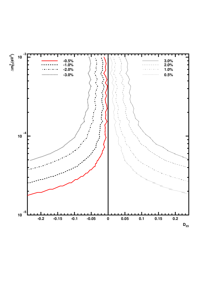
Figure 8: The contours of constant relative change of the number of the $e$-like events, $N_{e}^{osc}/N_{e}^{0}-1$ (in %), in the $\Delta m^{2}_{12}$ - $D_{23}$ plane. We take $\sin^{2}2\theta_{21}=0.82$ and $\sin\theta_{13}=0$.

The oscillation effect depends mainly on $\Delta m^{2}_{12}$ and $\sin^{2}\theta_{23}$. After precise determination of the $\Delta m^{2}_{12}$ (KamLAND will reach 10% accuracy and also SNO will contribute) one can use data on $N^{osc}_{e}/N^{0}_{e}$ in atmospheric neutrinos to search for deviation of 2-3 mixing from maximal. In fig. 8 we show contours of constant relative change of the $e$-like events in $\cos^{2}\theta_{23}-\Delta m^{2}_{12}$ plane. Notice that the lines are not symmetric with respect to $\cos^{2}\theta_{23}=0.5$ due to deviation of $r$ from 2. For this reason the bound from the side $\cos^{2}\theta_{23}<0.5$ is stronger. We assume here that $s_{13}\approx 0$. Uncertainties due to unknown values of $s_{13}$ and $\delta_{CP}$ will be discussed in sect IVC.

III.2 $U_{e3}$ induced interference

Let us assume that 1-3 mixing is non-zero but $\delta_{CP}=0$ (or $\pi$). Now all three terms in (41) give contributions to the oscillation effect. The interference term contribution is determined by the real part $R_{2}$. It dominates if the 2-3 mixing is close to maximal. In our estimations below we will use $\Delta m^{2}_{12}=7.3\cdot 10^{-5}$ eV² and $\sin^{2}2\theta_{12}\sim 0.82$.

In fig. 9 (upper panel) we show the zenith angle distribution of the total oscillation effect for different values of $s_{13}$ and $s^{2}_{23}=0.45$. The LMA contribution is positive and relatively small: its value averaged over the zenith angle equals $\epsilon_{e}^{LMA}=0.8\%$ (it is given by the line $s_{13}=0$, see the upper panel). The $U_{e3}$ contribution is also suppressed by the screening factor. It is negative for $s^{2}_{23}<0.5$, and being quadratic in $s_{13}$, does not depend on the sign of 1-3 mixing. We obtain

$$\epsilon^{Ue3}_{e}\approx-0.4\%\left(\frac{s_{13}}{0.16}\right)^{2}.$$ (49)

(Notice that there is a small matter effect on $s_{13}$ which is different in neutrino and antineutrino channel.)

The interference term is linear in $s_{13}$ and positive for the negative sign of $s_{13}$:

$$\epsilon^{int}_{e}=-2.0\%\left(\frac{s_{13}}{0.16}\right).$$ (50)

It can be estimated as follows. The depth of oscillations equals $\sim\sin 2\theta_{12}^{m}\cos 2\theta_{12}^{m}=0.47$. The averaging over $\cos\Theta_{\nu}$ gives $\langle R_{2}\rangle\sim 0.14$. Due to negative effect for antineutrinos the total effect is $\langle R_{2}\rangle\approx 0.09$. Averaging over the energy (which is important here) leads to further reduction by about 30 %. Finally we get $\epsilon^{int}_{e}=\langle R_{2}\rangle rs_{13}\approx 2\%$ for $s_{13}=-0.16$ in agreement with calculations.

Summing up all the contribution we find for $s_{13}=-0.16$: $\epsilon_{e}^{tot}=2.5\%$ in agreement with result in fig. 9 (upper panel). For $s_{13}=+0.16$, the interference term changes the sign and we get: $\epsilon_{e}^{tot}=-1.7\%$. Apparently the curves are not symmetric with respect to $N^{osc}_{e}/N^{0}_{e}=1$ due to the LMA- and $U_{e3}$- contributions which do not change the sign with $s_{13}$. When $|s_{13}|$ decreases, both $\epsilon^{int}_{e}$ and $\epsilon^{Ue3}_{e}$ decrease in absolute value.

In fig. 9 (lower panel) we show the zenith angle dependences for larger deviation of 2-3 mixing from maximal value, $s^{2}_{23}=0.35$. Now screening is weaker and the LMA oscillations give main contribution $\epsilon_{e}^{LMA}=2.9\%$. This leads to the shift of all the histograms to $N^{osc}_{e}/N^{0}_{e}>1$.

Now also the $U_{e3}$ contribution is larger being comparable with the interference contribution:

$$\epsilon^{Ue3}_{e}\approx-1.3\%\left(\frac{s_{13}}{0.16}\right)^{2}.$$ (51)

In contrast, the interference term has no screening factor and its absolute value even slightly decreases in comparison with the previous case due to decrease of $\sin^{2}2\theta_{23}$:

$$\epsilon^{int}_{e}=-1.9\%\left(\frac{s_{13}}{0.16}\right).$$ (52)

This leads to more complicated dependence of the excess on $s_{13}$. We find that maximum of total excess is realized for $s_{13}=-0.16$: $\epsilon_{e}^{tot}=3.6\%$. For $s_{13}=-0.08$ we get a very similar value: $\epsilon_{e}^{tot}=3.55\%$.

Maximal effect of interference can be estimated in the following way. As we have discussed, $R_{2}^{max}=1/2$ (which can be achieved at $\Delta m^{2}_{12}=7.3\cdot 10^{-5}$ eV²). The averaging over the zenith angle gives $\langle R_{2}\rangle=R_{2}^{max}/4=0.125$. The antineutrino contribution is negative, so that $\epsilon^{int}_{e}<2s_{13}(1-\xi)0.125=0.18s_{13}<3\%$. Averaging over the energy leads to an additional suppression.

Using curves which correspond to different sign of $s_{13}$, it is easy to disentangle contribution from the interference term. Obviously,

$$\epsilon^{int}_{e}(s_{13})=\frac{1}{2}\left[\epsilon_{e}^{tot}(s_{13})-\epsilon_{e}^{tot}(-s_{13})\right],$$ (53)

and for the two other contributions we get:

$$\epsilon_{e}^{LMA}=\epsilon_{e}^{tot}(s_{13}=0),~{}~{}~{}~{}~{}\epsilon^{Ue3}_{e}=\frac{1}{2}\left[\epsilon^{int}_{e}(s_{13})+\epsilon^{int}_{e}(-s_{13})\right]-\epsilon_{e}^{tot}(s_{13}=0).$$ (54)

In Fig. 10 we show dependence of the ratio of number of events integrated over the zenith angle, $N^{osc}_{e}/N^{0}_{e}$, on the energy. According to our analytical consideration, with decrease of energy the LMA contribution (green histogram) increases fast, the $U_{e3}$-contribution is unchanged and the interference term first, increases but then below $E\sim 0.4$ GeV starts to decrease. Using relations (53 - 54) we find from the Fig. 10 (upper panel) for $s_{13}=-0.16$ that in the bins $E=(0.4-0.65),~{}(0.25-0.40),~{}(0.10-0.25)$ GeV: $\epsilon_{e}^{LMA}=1.2\%,~{}~{}2.7\%,~{}~{}5.9\%$ respectively, $\epsilon^{Ue3}_{e}=-1.1\%=const$, whereas $\epsilon^{int}_{e}=1.7\%,~{}~{}2.7\%,~{}~{}2.4\%$. At high energies the interference term gives main contribution. (Notice, however, that for $E>0.6$ GeV our approximation may not be precise).

III.3 CP-violation effects

Let us consider effects of the CP-violating phase $\delta_{CP}$. Notice that if we substitute $I_{2}$ by its vacuum value (eq. (20) with $\theta_{m}\rightarrow\theta$), the interference term, as is expected, becomes equal $\epsilon^{int}_{e}=1/2\Delta P$, where $\Delta P$ is the neutrino-antineutrino CP- asymmetry.

According to fig. 4, $I_{2}$ alternates the sign with change of the zenith angle. However, there is no averaging of the effect to zero for two reasons:

1. For the mantle trajectories up to 1.5 - 2 periods of oscillations are obtained. In particular, for $2\cdot 10^{-4}$ eV²/GeV (fig. 4) which corresponds to the best value of $\Delta m^{2}_{12}$ and $E=0.4$ GeV there are 1.5 periods.

2. Due to change of the density for trajectories with different $\Theta_{e}$ the curves are not symmetric with respect to $I_{2}=0$.

For antineutrinos the probability $\bar{I}_{2}$ has smaller amplitude and oscillation length, furthermore, the curves are nearly symmetric with respect to $I_{2}=0$. As a results, integration over the zenith angles leads to strong suppression of the averaged value $\langle I_{2}\rangle$. This, as well as difference of the original neutrino and antineutrino fluxes result in existence of the CP-odd effects, even in the sample where neutrino and antineutrino signals are summed up.

In fig. 11 we show the zenith angle dependence of the oscillation effect for different values of $\delta_{CP}$. The analytical expression of this dependence on $\delta_{CP}$ is given in Eq. (37). Simple estimation of the effect can be obtained as follows. Using results of fig. 4 we obtain after averaging over the zenith angle and energies: $\langle I_{2}\rangle=0.040$ and $\langle\bar{I}_{2}\rangle\approx 0.018$. Then for $s_{13}=-0.16$ and $s_{23}^{2}=0.35$, the contribution of imaginary part to the interference term equals: $\epsilon_{I}^{int}\sim 1.1\%$. In the previous section we have found that for the same set of parameters $\epsilon_{R}^{int}\approx 2.0\%$. So, the interference effect can be written as

$$\epsilon_{e}^{int}\approx(2.0\cos\delta_{CP}-1.1\sin\delta_{CP})\%~{}~{}~{}~{}(s_{23}^{2}=0.35).$$ (55)

The relative values of numerical coefficients depend on the $2\nu$ probabilities $R_{2}$ and $I_{2}$. For $\delta_{CP}=-\pi/4$ we find $\epsilon_{e}^{int}\approx 2.2\%$ (no change with respect to $\delta_{CP}=0$). For $\delta_{CP}=\pi/2$: $\epsilon_{e}^{int}=\epsilon_{I}^{int}\approx 1.1\%$. Maximal effect of $I_{2}$ is for $\delta_{CP}=-\pi/2$: $\epsilon_{e}^{int}=\epsilon_{I}^{int}\approx 1.1\%$, that is, the excess decreases by $2.8\%$ in comparison with $\delta_{CP}=0$ case (see fig. 11 upper panel). From fig. 9 and relations (53 - 54) we find $\epsilon_{e}^{LMA}+\epsilon^{Ue3}_{e}\approx 2.2\%$, and consequently,

$$\epsilon_{e}^{tot}=2.2\%+\epsilon_{e}^{int}.$$ (56)

The latter formula reproduces well the results shown in fig. 11.

Let us compare different contributions to the excess of the $e$-like events. As we have established the largest contribution can be obtained from the LMA term. Maximum of $\epsilon^{LMA}_{e}\sim 6\%$ is achieved for the largest possible $\Delta m^{2}_{12}$, minimal energy and largest deviation of the 2-3 mixing from maximum. The contribution does not depend on $s_{13}$.

The interference term gives maximal contribution, $\epsilon^{int}_{e}\sim 3\%$, for $\Delta m^{2}_{12}=7\cdot 10^{-5}$ eV² and maximal possible value $s_{13}$. It depends very weakly on the deviation $D_{23}$.

The $U_{e3}$ maximal contribution, $\epsilon^{Ue3}_{e}\sim 1-2\%$, is realized for the largest possible values of $s_{13}$ and $D_{23}$. It does not depend on $\Delta m^{2}_{12}$ in the first approximation. According to (36) this term has an opposite sign with respect to the LMA term and therefore partial cancellation with the LMA contribution always occurs.

These results allow one to understand that the contributions of non-zero $s_{13}$ (interference term and $U_{e3}$) can not further enhance the excess produced by the LMA term. Indeed, for large $\Delta m^{2}_{12}\sim 2\cdot 10^{-4}$ eV² where $\epsilon^{LMA}_{e}$ is maximal, the interference term contribution is already small, and moreover, the $U_{e3}$ term is negative compensating substantially the positive $\epsilon^{int}_{e}$ contribution. As a result the LMA contribution can be enhanced by about $1\%$ at most. For $\Delta m^{2}_{12}\sim 7\cdot 10^{-5}$ eV² where the interference term is maximal, the LMA contribution is smaller and again partial cancellation with $U_{e3}$ contribution occurs.

Notice that the cancellation of the LMA induced excess can be stronger than the enhancement since $\epsilon^{int}_{e}$ and $\epsilon^{Ue3}_{e}$ can have both the same negative sign with respect to $\epsilon^{LMA}_{e}$.

IV Measuring $D_{23}$ and $\delta_{CP}$

In terms of the deviation parameter (38) the excess of the $e$-like events can be written as

$$\epsilon_{e}=r\left(\langle P_{2}\rangle-2\tilde{s}_{13}^{2}\right)D_{23}+\epsilon^{int}_{e}+(r/2-1)\left(\langle P_{2}\rangle+2\tilde{s}_{13}^{2}\right).$$ (57)

The interference term depends on the deviation very weakly: $\epsilon^{int}_{e}\propto\sin 2\theta_{23}=\sqrt{1-4D_{23}^{2}}\approx 1-2D_{23}^{2}$. Since variations of $D_{23}$ in the presently allowed range (39) change $\epsilon^{int}_{e}$ by less than 5% and in the first approximation this dependence can be neglected. Also the last term in (57) does not exceed 0.5 %. Therefore with a good approximation $\epsilon_{e}$ is a linear function of $D_{23}$. We can find coefficients of this function using fig. 9.

For $\Delta m^{2}_{12}\sim 7\cdot 10^{-5}$ eV² and zero 1-3 mixing we get

$$\epsilon_{e}^{0}\approx(20.5D_{23}-0.3)\%.$$ (58)

For $|s_{13}|=0.16$ maximal (corresponds to $s_{13}=-0.16$) and minimal ($s_{13}=0.16$) values of $\epsilon_{e}$ can be approximated as

$$\epsilon_{e}^{max}=(12.5D_{23}+1.8)\%,~{}~{}~{}~{}\epsilon_{e}^{min}=(12.8D_{23}-2.1)\%.$$ (59)

Since for the present upper limit on $D_{23}$, $\epsilon_{e}^{min}(0.15)<0$, any upper experimental bound, $\epsilon_{e}^{exp}$, will not improve the limit for $D_{23}$ (39).

If the lower bound on $\epsilon_{e}$ is established, one can put the lower bound on $D_{23}$. Using expression for $\epsilon_{e}^{max}$ we find that the lower bounds $\epsilon_{e}^{exp}>2\%$, and $\epsilon_{e}^{exp}>3\%$ will give $D_{23}>0.02$ and $D_{23}>0.10$ correspondingly.

The bound on $D_{23}$ can be improved if future experiments put stronger bound on $s_{13}$. For $|s_{13}|=0.08$ maximal and minimal values of $\epsilon_{e}$ equal

$$\epsilon_{e}^{max}\approx(17D_{23}+0.84)\%,~{}~{}~{}~{}\epsilon_{e}^{min}\approx(18.5D_{23}-1.2)\%.$$ (60)

From the expression for $\epsilon_{e}^{min}$ we find that the present bound on $D_{23}$ will be improved provided that the upper bound on the excess is better than 1.6 %. If $\epsilon_{e}^{exp}<1\%$, we get $D_{23}<0.1$ etc..

Using $\epsilon_{e}^{max}$ we obtain that the lower experimental bound $\epsilon_{e}^{exp}>2\%$ will lead to the lower bound $D_{23}>0.07$.

Suppose very strong bound on $s_{13}$ is obtained and the lower bound $\epsilon_{e}^{exp}>0.02$ will be established. Then according to fig. 8 the interval $\Delta m^{2}_{12}=(7.3\pm 0.7)\cdot 10^{-5}$ eV² (10% error) will lead to the lower bound on deviation from maximal mixing $D_{23}>0.1$.

Can the CP-violation phase be measured? As follows from the fig.  11, the phase $\delta_{CP}$ does not produce any particular zenith angle dependence and the energy dependence (not showed). The same effect can be achieved by changing other parameters.

Let us consider the most favorable case: $\Delta m^{2}_{12}\sim 7.3\cdot 10^{-5}$ eV² and $|s_{13}|\sim 0.16$. The total relative change of number of the e-like events can be written as

$$\epsilon_{e}=(1.8\cos\delta_{CP}-0.8\sin\delta_{CP})+13.6D_{23}~{}\%.$$ (61)

Depending on $\delta_{CP}$ the interference term changes in the limits $-1.92\div+1.92$. The LMA contribution is restricted by $|\epsilon^{LMA}_{e}|\approx 13.6|D_{23}|\leq 2.04\%$. So, the predictions can be in the interval $-3.96\div+3.96$.

On the other hand, for $\delta_{CP}=0$, $|\epsilon^{int}_{e}|=1.8\%$. Therefore for zero CP-violating phase the excess (deficiency) can be in the intervals: $(0.2\div 3.8)\%$ and $(-3.8\div-0.2)\%$ which covers practically whole the interval predicted for non-zero CP-violating phase. So, to get any information about $\delta_{CP}$ one needs to improve the bound on the deviation $D_{23}$ from independent measurements. From fig. 6 it follows that

$$\Delta\epsilon_{e}=-2\%\cdot\frac{\Delta(\sin^{2}\theta_{23})}{0.1}.$$ (62)

E.g., 1% effect of $\delta_{CP}$ can be produced also by 0.05 change of $\sin^{2}\theta_{23}$: from 0.35 to 0.40. Variations by 3% would require the increase of $\sin^{2}\theta_{23}$ from 0.35 to 0.5.

Apparently, the effect similar to that of $\delta_{CP}$ can be produced also by small variations of $s_{13}$, or $\Delta m^{2}_{12}$. Let us consider this degeneracy of parameters.

Using fig. 5 (upper panel) we find that change of the excess by 1% can be achieved by (35 - 40)% change of $\Delta m_{12}^{2}$ near the best fit point, e.g., from 5.2 to $8.7\cdot 10^{-5}$ eV²:

$$\Delta\epsilon_{e}=0.44\%\cdot\frac{\Delta(\Delta m_{12}^{2})}{10^{-5}{\rm eV}^{2}}$$ (63)

(for $\sin^{2}_{23}=0.35$). The effect is smaller if the 2-3 mixing is closer to maximum. $\Delta\epsilon_{e}=1$% would require rather large change of $\Delta m_{12}^{2}$: from 5 to 15 of $10^{-5}$ eV².

Further operation of the KamLAND and SNO will allow to determine $\Delta m_{12}^{2}$ with 10% ambiguity, which is transferred in 0.3% ambiguity in $\epsilon_{e}$.

The degeneracy of the $\delta_{CP}$ and $s_{13}$ is more complicated and it depends on specific value and sign of $s_{13}$ as well as $\sin^{2}\theta_{23}$. In particular, for $\sin^{2}\theta_{23}=0.35$ and $s_{13}=-0.16$ the dependence of $\epsilon_{e}$ on $s_{13}$ is rather weak (fig. 9): A reduction of the excess by 1% requires increase of $s_{13}$ from - 0.16 to + 0.05. For $\sin^{2}\theta_{23}=0.45$, $\Delta\epsilon_{e}=1\%$ can be compensated by changes of $s_{13}$ in the interval $-0.22\div-0.10$. That is, moderate accuracy of measurements of $s_{13}$ could be enough to determine $\delta_{CP}$. Notice, however, that with decrease of $s_{13}$ the effect of $\delta_{CP}$ decreases.

Dependence of the oscillation effect on 1-2 mixing is very weak: variations of $\tan^{2}\theta_{12}$ in the interval from 0.30 to 0.52 produce a change $\Delta\epsilon_{e}=0.3\%$. Expected improvements of determination of $\tan^{2}\theta_{12}$ will further reduce this ambiguity.

The main problem is the identification and measurement (or restriction) of the oscillation effect in view of large present uncertainties in the original neutrino flux (15 - 20 %). In principle, if high enough statistics will be achieved the oscillation effect can be distinguished from the renormalization by its zenith angle and energy dependences. At the same time, further improvements in the calculations of the neutrino fluxes are extremely important. Also separate measurements of the neutrino and antineutrino signals will help.

V Conclusion

1. After confirmation of the LMA MSW solution of the solar neutrino problem it is clear that the effect of $\nu_{e}$ - oscillations should appear in the atmospheric neutrinos at some level even for zero value of $s_{13}$.

For the allowed values of the oscillation parameters, in particular, $\sin^{2}2\theta_{23}>0.91$, the LMA oscillations can produce the integrated effect (excess or deficit) up to (5 - 6) % in the sub-GeV sample. The effect increases with decrease of energy and in the low energy part of the sample it can be as large as 8%. The zenith angle dependence of the effect is rather weak with maximum achieved in the upward-going bins.

The LMA effect is strongly suppressed for exactly maximal 2-3 mixing, so searches for the oscillation effect in the sub-GeV sample can be used to measure the deviation of 2 - 3 mixing from maximum. Here, however, an ambiguity appears due to unknown values of $s_{13}$ and $\delta_{CP}$. The ambiguity can be reduced if stronger bound on $s_{13}$ will be established from independent measurements.

2. The present experimental accuracy is comparable with the maximal expected effect. Notice that without additional renormalization of the original neutrino fluxes, the data show some excess of the $e$-like events which can be explained (at least partially) by the LMA-oscillations. In fact, the data (including weak zenith angle and energy dependences of the excess can be perfectly reproduced by the LMA-contribution corresponding to the best fit values of parameters and partial (3- 5%) renormalization of spectrum.

The excess of $e$-like events in the sub-GeV sample and the absence of the excess in the multi-GeV range (as it is indicated by the present data) testify for the deviation of the 2-3 mixing from maximum.

3. Non-zero 1-3 mixing gives an additional contribution to the oscillation effect. For the sub-GeV sample, it leads to interference of the the two neutrino amplitudes driven by solar oscillation parameters (induced interference). The interference term is linear in $s_{13}$ and does not contain the screening factor. It dominates if 2-3 mixing is close to maximal.

The interference term can reach 2 - 3%. The maximal value (real part) corresponds to $\Delta m_{12}^{2}\approx 7\cdot 10^{-5}$ eV² for the sub-GeV sample.

The 1-3 mixing leads also to contribution proportional to $s_{13}^{2}$ which does not exceed $\sim 1\%$.

4. The interference term depends on the CP-violating phase $\delta_{CP}$. Variations of $\delta_{CP}$ can change the oscillation effect by $|\Delta\epsilon|=3$%.

5. The relative effects of $\delta_{CP}$ is enhanced for the sample induced by neutrinos or antineutrinos, that is, when the sign of the electric charge of electron is identified.

6. Various contributions to the oscillation effect have slightly different zenith angle and also energy dependences. This, in principle, can be used to separate them. In particular, the LMA-contribution increases with decrease of the energy, the interference term first increases and then starts to decrease.

The zenith angle dependence is very weak for low energy bins.

7. There is strong “degeneracy” of parameters once total excess is measured only. The same integral oscillation effect can be produced for different values of $\sin^{2}\theta_{23}$, $\Delta m^{2}_{12}$, $s_{13}$ and $\delta_{CP}$.

8. In principle, future high statistics studies of the atmospheric neutrinos will allow to measure the neutrino oscillation parameters. For this the accuracy of measurements of the oscillation effect should be about 1% or better. Also a way should be found to distinguish the oscillation effect from the effect of the neutrino flux normalization. The problem of degeneracy of parameters should be resolved. There is a good chance to measure $\Delta m^{2}_{12}$ with high enough accuracy, so that the corresponding uncertainty will be eliminated. It will be very difficult to resolve ambiguity related to of $\sin^{2}\theta_{23}$, $s_{13}$ and $\delta_{CP}$. If future (e.g., reactor) experiments put stronger bound on $s_{13}$, the ambiguity related to $s_{13}$ and $\delta_{CP}$ can be substantially reduced. This will allow to use the atmospheric data to restrict a deviation of the 2-3 mixing from the maximal one.

9. With present knowledge of the oscillation parameters, one can expect the effect of $\nu_{e}$ oscillations at the level of existing experimental error bars and uncertainties in the normalization of fluxes. The effect of the LMA oscillations should be taken into account in the analysis of the atmospheric neutrino data.

Appendix

Let us evaluate the effect of the interference between the solar and the atmospheric frequencies we have neglected in our consideration. This interference gives additional terms to the probabilities $P_{\mu e}$ (19) and $P_{ee}$ (22):

$$\Delta P_{\mu e}=-2\tilde{s}_{13}^{2}\tilde{c}_{13}^{2}s_{23}^{2}K_{ee}+2\tilde{s}_{13}\tilde{c}_{13}^{2}s_{23}c_{23}K_{\mu e},$$ (64)

$$\Delta P_{ee}=2\tilde{s}_{13}^{2}\tilde{c}_{13}^{2}K_{ee},$$ (65)

where

$$K_{ee}\equiv Re\left[\tilde{A}_{ee}^{*}\tilde{A}_{\tau\tau}\right],~{}~{}~{}K_{\mu e}=Re\left[\tilde{A}_{\mu e}^{*}e^{i\delta_{CP}}\tilde{A}_{\tau\tau}\right],~{}~{}~{}$$ (66)

Notice that $K_{\mu e}$ depends on the CP-violating phase. Inserting (64) and (65) in (35) we get the corresponding corrections to the relative change of number of the $e$-like events:

$$\Delta\epsilon_{e}=2\tilde{s}_{13}^{2}\tilde{c}_{13}^{2}(1-rs_{23}^{2})\langle K_{ee}\rangle+2r\tilde{s}_{13}\tilde{c}_{13}^{2}s_{23}c_{23}\langle K_{\mu e}\rangle.$$ (67)

Here $\langle...\rangle$ denotes the averaging over the energy and the zenith angle.

Let us evaluate two terms in this equation in order.

1). The first term is proportional to two small factors: $s_{13}^{2}D_{23}<0.015$. For trajectories with $\cos\Theta>0$ taking $\tilde{A}_{ee}\approx 1$ we estimate: $\langle K_{ee}\rangle<\langle\cos\Phi_{3}\rangle$. Since for typical energy 0.4 GeV, the oscillation length in vacuum is $l_{13}\sim 500$ km, and the phase equals $\Phi_{3}\sim 2\pi$. Therefore averaging over the zenith angle and the energy lead to strong suppression: $\langle K_{ee}\rangle\sim 0.2$. As a result, the whole term is smaller than 0.3%.

2). In the second term of (67) $\langle K_{\mu e}\rangle$ can be estimated in the following way. In vacuum:

$$\tilde{A}_{\mu e}=-s_{12}c_{12}\left(1-e^{-i\phi_{2}}\right),~{}~{}~{}\phi_{2}=\frac{\Delta m_{12}^{2}L}{2E}.$$ (68)

For trajectories with $\cos\Theta>0$ the phase driven by the solar mass split is small: $\phi_{2}<0.2$, so that

$$\langle K_{\mu e}\rangle\approx-s_{12}c_{12}\langle\phi_{2}\sin(\phi_{3}+\delta_{CP})\rangle=-s_{12}c_{12}\langle\frac{2\pi d}{l_{12}}\frac{1}{\cos\Theta}\sin(\phi_{3}+\delta_{CP})\rangle,$$ (69)

where $d\sim 20$ km is the depth of the atmosphere. For $E=0.4$ GeV the oscillation length equals $l_{12}=1.4\cdot 10^{4}$ km. The averaging over the zenith angle gives $\langle 1/\cos\Theta\rangle=3.2$. Then taking $\sin(\phi_{3}+\delta_{CP})=1$ we obtain from (69)

$$|\langle K_{\mu e}\rangle|<3\cdot 10^{-2}s_{12}c_{12},$$ (70)

and consequently, for $s_{13}\leq 0.16$ the contribution of the second term to $\Delta\epsilon_{e}<0.5\%$. Averaging over the energy leads to further suppression of this contribution.

Figure 5: Zenith angle distributions of the $e$-like sub-GeV events for $\sin\theta_{13}=0$. The ratio of the numbers of events with and without $\nu_{e}$-oscillations, $N_{e}^{osc}/N_{e}^{0}$, for different values of $\Delta m^{2}_{12}$. From the upper to lower histograms the corresponding value of $\Delta m^{2}_{12}$ decreases. We take $\sin^{2}2\theta_{12}=0.82$ and $\sin^{2}\theta_{23}=0.35$ (upper panel), $\sin^{2}\theta_{23}=0.45$ (lower panel). Shown are also the Super-Kamiokande experimental points from Ref. super-data-used .

Figure 6: Zenith angle distributions of the $e$-like sub-GeV events for $\sin\theta_{13}=0$. The ratio of numbers of events with and without $\nu_{e}$-oscillations, $N_{e}^{osc}/N_{e}^{0}$, for different values of $\sin^{2}\theta_{23}$. We take $\sin^{2}2\theta_{12}=0.82$ and $\Delta m^{2}_{12}=7.3\cdot 10^{-5}$ eV². From the upper to lower histograms the corresponding value of $\sin^{2}\theta_{23}$ increases. Shown are also the Super-Kamiokande experimental points from Ref. super-data-used .

Figure 7: The excess of the $e$- like events integrated over the zenith angles as a function of energy. Dependence of the ratio of numbers of the $e$-like sub-GeV events with and without $\nu_{e}$-oscillations, $N_{e}^{osc}/N_{e}^{0}$, on the visible energy for different values of $\Delta m^{2}_{12}$. From the upper to lower histograms the corresponding value of $\Delta m^{2}_{12}$ decreases. For other parameters we take: $\sin^{2}2\theta_{12}=0.82$, $\sin^{2}\theta_{23}=0.35$ and $\sin\theta_{13}=0$. Shown are also the Super-Kamiokande experimental points from Ref. super-data-used .

Figure 9: Zenith angle distributions of the sub-GeV $e$-like events for non-zero 1-3 mixing. The ratio of the numbers of events with and without $\nu_{e}$ oscillations for different values of $\sin\theta_{13}$. We take $\sin^{2}2\theta_{12}=0.82$, $\Delta m^{2}_{12}=7.3\cdot 10^{-5}$ eV² and $\sin^{2}\theta_{23}=0.45$ (upper panel), and $\sin^{2}\theta_{23}=0.35$ (lower panel). The excess increases with decrease of $\sin\theta_{13}$. Shown are also the Super-Kamiokande experimental points from Ref. super-data-used .

Figure 10: The excess of the $e$- like events integrated over the zenith angles as a function of energy. Dependence of the ratio of number of $e$-like events with oscillations and without oscillations on the visible energy for different values of $\sin\theta_{13}$. For other parameters we take: $\sin^{2}2\theta_{23}=0.91$ and $\Delta m^{2}_{12}=7.3\cdot 10^{-5}$ eV². The excess increases with decrease of $\sin\theta_{13}$. Shown are also the Super-Kamiokande experimental points from Ref. super-data-used .

Figure 11: Zenith angle distributions of the sub-GeV $e$-like events for non-zero 1-3 mixing. The ratio of the numbers of events with and without $\nu_{e}$ oscillations for different values of the CP-violating phase $\delta_{CP}$. We take $\sin^{2}\theta_{23}=0.35$, $\sin^{2}2\theta_{12}=0.82$, $\sin\theta_{13}=0.16$, $\Delta m^{2}_{12}=7.3\cdot 10^{-5}$ eV². In the upper (lower) panel, the excess decreases (increases) with increase of $\delta_{CP}$. Shown are also the Super-Kamiokande experimental points from Ref. super-data-used .

References

- (1) Super-Kamiokande Collaboration, S. Fukuda, et al., Phys. Rev. Lett. 85, 3999 (2000).
-
(2)
Super-Kamiokande Collaboration,
Y. Hayato talk given at the
EPS 2003 conference (Aachen, Germany, 2003, transparencies available at
http://eps2003.physik.rwth-aachen.de/ - (3) Soudan 2 Collaboration, W. W. M. Allison et al., Phys. Lett. B 391, 491 (1997); Soudan 2 Collaboration, M. Sanchez et al., hep-ex/0307069.
- (4) MACRO Collaboration, Phys. Lett. B566 35, (2003).
- (5) K2K Collaboration, M. H. Ahn et al. Phys. Rev. Lett. 90, 041801 (2003).
- (6) I. Mocioiu and R. Shrock, JHEP 0111, 50 (2001). G.L. Fogli, E. Lisi, A. Marrone and D. Montanino Phys. Rev. D67, 093006 (2003). M.C. Gonzalez-Garcia, M. Maltoni, Eur.Phys.J. C26, 417 (2003);
- (7) KamLAND Collaboration, K. Eguchi et al., Phys. Rev. Lett, 90, 021802 (2003).
- (8) SNO Collaboration, Q. R. Ahmad, et al., nucl-ex/0309004.
- (9) O. Yasuda, hep-ph/9602342; hep-ph/9706546.
- (10) R. P. Thun and S.Mckee, Phys. Lett. B439, 123 (1998).
- (11) G. L. Fogli, E. Lisi, A. Marrone and G. Scioscia, Phys. Rev. D59, 033001 (1998).
- (12) C. W. Kim, U. W. Lee, Phys. Lett. B444, 204 (1998).
- (13) T. Teshima, T. Sakai, Prog.Theor.Phys. 102, 629 (1999).
- (14) J. Bunn, R. Foot and R. R. Volkas, Phys. Lett. B413, 109 (1997).
- (15) O.L.G. Peres and A.Yu. Smirnov, Phys. Lett. B456, 204 (1999).
- (16) M. C. Gonzalez-Garcia and M. Maltoni, Eur. Phys. J. C 26, 417 (2003).
- (17) M. Honda et al., Phys. Lett. B248, 193 (1990); idem, Phys. Rev. D52, 4985 (1995).
-
(18)
A. Kobayashi, PhD Thesis, University of
Hawaii, Aug. 2002. Available at
http://www-sk.icrr.u-tokyo.ac.jp/doc/sk/pub/atsuko.ps.gz. -
(19)
Y. Totsuka, for the Super-Kamiokande
Collaboration, talk presented at TAUP 2001
Topics in Astroparticle and Underground Physics
September 8-12, 2001, Assergi, Italy. Transparencies available at
http://taup2001.lngs.infn.it/. - (20) BESS Collaboration, T.Sanuki et al., Astrop. J.545 1135(2000).
- (21) AMS Collaboration, J. Alcaraz et al., Phys. Lett. B490 27 (2000).
- (22) G. Battistoni et al., Astr. Part. 12, 315(2000); M. Honda et al., Phys. Rev. D64, 053011 (2001); G. Battistoni, A. Ferrari, T. Montaruli and P. R. Sala, arXiv:hep-ph/0305208.
- (23) J. Pantaleone, Phys. Rev. D49, 2152 (1994); G. L. Fogli, E. Lisi, D. Montanino, Astropart. Phys. 4, 177 (1995); G. L. Fogli, E. Lisi, D. Montanino, G. Scioscia, Phys. Rev. D55, 4385 (1997); G. L. Fogli, E. Lisi, A. Marrone, ibid D57, 5893 (1998); O. Yasuda, ibid D58, 091301(1998); J. Pantaleone, Phys. Rev. Lett. 81, 5060 (1998).
- (24) C. Giunti, C. W. Kim, J. D. Kim, Phys. Lett. B352, 357 (1995); P. F. Harrison, D. H. Perkins, ibid B349, 137 (1995); idem B396, 186 (1997); H. Fritzsch, Z.-Z. Xing, ibid B372, 265 (1996); C. Giunti, C. W. Kim, M. Monteno, Nucl. Phys. B521, 3 (1998); R. Foot, R. R. Volkas, O. Yasuda, Phys. Lett. B421, 245 (1998) ; ibid B433, 82(1998).
- (25) G. L. Fogli, E. Lisi, A. Marrone, D. Montanino, Phys. Lett. B425, 341 (1998).
- (26) G. L. Fogli, E. Lisi, D. Montanino, Phys. Rev. D49, 3626 (1994); G. L. Fogli, E. Lisi, G. Scioscia, ibid D52, 5334 (1995); S. M. Bilenkii, C. Giunti, C. W. Kim, Astropart. Phys. 4, 241 (1996); O. Yasuda, H. Minakata, hep-ph/9602386; Nucl.Phys. B523, 597 (1998); Phys. Rev. D56, 1692 (1997); T. Teshima, T. Sakai, O. Inagaki, Int.J.Mod.Phys. A14 1953 (1999); T. Teshima, T. Sakai, Prog. Theor. Phys. 101 147 (1999); V. Barger, S. Pakvasa, T. J. Weiler, K. Whisnant, Phys. Lett. B437, 107(1998); R. Barbieri, L. J. Hall, D. Smith, A. Strumia, N. Weiner, JHEP 9812 017 (1998); V. Barger, T. J. Weiler, K. Whisnant, Phys. Lett. B440 1(1998).
- (27) E. Kh. Akhmedov, A. Dighe, P. Lipari, A. Yu. Smirnov, Nucl. Phys. B542, 3 (1999).
- (28) J.J. Gomez-Cadenas and M.C. Gonzalez-Garcia, Z. Phys. C71, 443(1996); V. Barger, T.J. Weiler and K. Whisnant, Phys. Lett. B427, 97(1998); V. Barger, S. Pakvasa, T.J. Weiler, K. Whisnant, ibid D58, 093016(1998).
- (29) J. Bernabeu, S. Palomares Ruiz and S. T. Petcov, Nucl. Phys. B 669, 255 (2003).
- (30) M. C. Gonzalez-Garcia and C. Pena-Garay, arXiv:hep-ph/0306001.
- (31) M. Maltoni, T. Schwetz, M. A. Tortola and J. W. Valle, arXiv:hep-ph/0309130.
- (32) CHOOZ Collaboration, M. Apollonio et al., Phys.Lett. B420, 397 (1998); M. Apollonio et al., Eur. Phys. J. C 27, 331 (2003).
- (33) O.L.G.Peres and A.Yu. Smirnov, Nucl. Phys. Proc.Suppl. 110, (2002).
- (34) E. Lisi and D. Montanino, Phys. Rev. D56, 1792 (1997).
- (35) V. Agrawal et al., Phys. Rev. D53, 1314 (1996); T. K. Gaisser and T. Stanev, ibid D57, 1977 (1998).
- (36) P. Lipari, M. Lusignoli, and F. Sartogo, Phys. Rev. Lett. 74, 4384 (1995).
- (37) M. C. Gonzalez-Garcia, H. Nunokawa, O. L. G. Peres, T. Stanev, J. W. F. Valle, Phys. Rev. D58, 033004 (1998).