CERN-TH/2003-230

Universal features of JIMWLK and BK evolution at small $x$

Kari Rummukainen$,^{1,2}$ and Heribert Weigert³

¹ CERN, Theory division, CH-1211 Geneva 23, Switzerland
² Department of Physics, University of Oulu, P.O.Box 3000, FIN-90014 Oulu, Finland
³ Institut für theoretische Physik, Universität Regensburg, 93040 Regensburg, Germany

In this paper we present the results of numerical studies of the JIMWLK and BK equations with a particular emphasis on the universal scaling properties and phase space structure involved. The results are valid for near zero impact parameter in DIS. We demonstrate IR safety due to the occurrence of a rapidity dependent saturation scale $Q_{s}(\tau)$. Within the set of initial conditions chosen both JIMWLK and BK equations show remarkable agreement. We point out the crucial importance of running coupling corrections to obtain consistency in the UV. Despite the scale breaking induced by the running coupling we find that evolution drives correlators towards an asymptotic form with near scaling properties. We discuss asymptotic features of the evolution, such as the $\tau$- and $A$-dependence of $Q_{s}$ away from the initial condition.

1 Introduction

With the advent of modern colliders, from the Tevatron, HERA to RHIC and planned experiments like LHC and EIC, the high energy asymptotics of QCD has gained new prominence and importance. The question if QCD effects there show universal features that might be calculated without recourse to intrinsically non-perturbative methods capable of also dealing with large $\alpha_{s}$ has gained new importance. In situations in which the experimental probes see large gluon densities at small $x$ the answer to this question has, maybe surprisingly, turned out to be positive. The progress has come from a method that resums the “density” induced corrections exactly while treating other effects, such as the $x$ dependence as perturbative corrections. The justification for this is that the density effects induce a generally $x$ dependent correlation length $1/Q_{s}(x)$ which also sets the scale for the coupling, thus giving us a small expansion parameter. There are several properties of the interactions at small $x$ that allow us to perform such a resummation. To explain them let us consider the simplest example of a $\gamma^{*}A$ collision, deep inelastic scatting (DIS) of virtual photons off nuclear targets, be it protons or larger nuclei. Generalizations to diffraction, $pA$ and $AA$ scattering are possible and share many of the key features.

Thus we are considering a collision of a virtual photon that imparts a (large) space-like momentum $q$ ($Q^{2}:=-q^{2}$ is large) on a nucleus of momentum $p$. At large energies the only other relevant invariant is Bjorken $x$ with $x:=\frac{Q^{2}}{2p.q}$. A leading twist analysis of DIS employing an OPE based on the largeness of $Q^{2}$ allows us to express the the cross section entirely in terms of two point functions, the quark and gluon distributions. At the same time it becomes possible to calculate their $Q^{2}$ dependence to leading logarithmic accuracy (summing corrections of the form $(\alpha_{s}\ln Q^{2})^{n}$) by solving the DGLAP equations. This amounts to summing the well-known QCD ladder diagrams. This procedure is self consistent and perturbatively under control as long as we stay within the large $Q^{2}$ region. Starting from a large enough $Q^{2}$ and going to larger values, we find that the objects we count with the quark and gluon distributions increase in number but they stay dilute: their “sizes” follow the transverse resolution scale $1/Q$. At small $x$, however, the growth of the gluon distribution is particularly pronounced and any attempt to resum corrections of the form $(\alpha_{s}\ln(1/x))^{n}$) to track the $x$-dependence of the cross sections immediately is faced with extreme growth of gluon distributions: moving towards small $x$ at fixed $Q^{2}$ increases the number of gluons of fixed “size” $1/Q$, so that the objects resolved will necessarily start to overlap. This is depicted in Fig. 1.

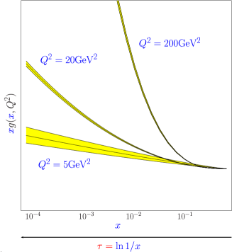
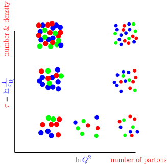
Figure 1: Gluon distributions grow towards small $x$. To the left: qualitative growth as from typical DGLAP fits of DIS at HERA ($eA$) for different $Q^{2}$. To the right: Growth of gluon (parton) numbers with $Q^{2}$ and $\ln(1/x)$. Going to sufficiently small $x$ at fixed $Q^{2}$ partons start to overlap.

At this point we have long since left the region in which an OPE treatment at leading twist is meaningful. Instead of single particle properties like distribution functions we need to take into account all higher twist effects that are related to the high density situation in which the gluons in our target overlap. At small $x$ we are thus faced with a situation in which we clearly need to go beyond the standard tools of perturbative QCD usually based on a twist expansion.

There are different ways to isolate the leading contributions to the cross section at small $x$ in a background of many or dense gluons and the history of the field is long [1, 2, 3, 4, 5, 6, 7, 8, 9, 10, 11, 12, 13, 14, 15, 16, 17, 18, 19, 20, 21, 22, 23, 24]. We will use a physically quite intuitive picture first used in the formulation of the McLerran-Venugopalan model, a formulation that was originally given in the infinite momentum frame of the nuclear target. Probing this target at small $x$ implies a large rapidity difference $\tau=\ln(1/x)$ between projectile and target, corresponding to a large relative boost factor $e^{\tau}$. Knowing from the above considerations that the interaction will be dominated by gluonic configurations we try to isolate the boost enhanced ones. Looking at the gluon field strength of the target for that purpose we find that $F^{+i}$ components are boost enhanced, while all others are left small and can, for our purposes, be set to zero. At the same time we find a strong Lorentz contraction, which we take to be in $x^{-}$ direction, and a time dilation, correspondingly in $x^{+}$ direction. With such a field strength tensor there we are left with only one important degree of freedom which, by choice of gauge, can be taken to be the + component of a gauge field. Taking into account time dilation and Lorentz contraction the gauge field can then be written as

$$\begin{split}A=&b+\delta A\qquad\mbox{with}\qquad b^{i,-}=0,\quad b^{+}=\beta(\bm{x})\delta(x^{-})\ .\end{split}$$ (1)

where the leading contribution $b^{+}$ is $x^{+}$ independent and Lorentz contracted to a $\delta$-function. Both of these are to be taken to be true with a resolution imposed by the rapidity separation $\tau=\ln(1/x)$. Note that mathematically we can always trade a gauge field that has only a single component for a path ordered exponential along the direction that picks up this component:

$$b^{+}=i(\partial^{+}U)U^{\dagger}\hskip 28.45274ptU={\sf P}\exp-i\int\!\!dz^{-}b^{+}(z^{-},{\bm{x}},0)$$ (2)

If multiple eikonal interactions are relevant as the high energy nature of the process would suggest, we expect these path ordered exponentials to be the natural degrees of freedom.

Ignoring the small fluctuations $\delta A$ for a moment we have a picture in which the $\gamma^{*}$ cross section arises from a diagram in which the photon splits into a $q\bar{q}$ pair which then interacts with the background field. Due to the $\delta$ like support of $b^{+}$ the $q\bar{q}$ are not deflected in the transverse direction during that interaction. This just reflects the largeness of the longitudinal momentum component of these partons at small $x$. This is shown in Fig. 2. To be sure, the physics content is not frame dependent although it is encoded differently in, say the rest frame of the target. There, we see neither Lorentz contraction nor time dilation. However the scale relations are preserved: the photon splits into a $q\bar{q}$ pair far outside the target and its $p^{-}$ is so large that typical $x^{+}$ variations of the target are negligible during the interaction. As a consequence the probe is not deflected in the transverse direction, picking up any multiple interactions with (gluonic) scattering centers as it punches though the target. This is shown in Fig. 2.

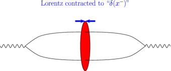
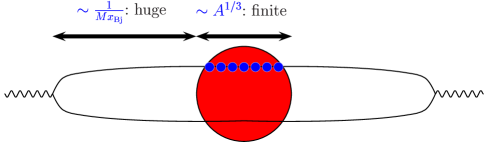
Figure 2: $q\bar{q}$ pairs interacting with a nuclear target at small $x$. (a) shows the situation in the targets infinite momentum frame with fully Lorentz-contracted target fields, (b) shows the situation in the target rest frame in which the $\gamma^{*}q\bar{q}$ vertex is far outside the target at a distance proportional to $1/x=e^{\tau}$.

That multiple interactions are of relevance immediately becomes obvious once we try to calculate such diagrams with a background field method. To this end we calculate the diagram shown in Fig. 2 in the background of a field of the type shown in Eq. (1) ignoring the small fluctuations. This immediately leads to the expression

$$\sigma_{\mathrm{DIS}}(x_{\mathrm{Bj}},Q^{2})=\text{\cal Im}\ \begin{minipage}[c]{85.35826pt} \includegraphics[height=22.76228pt]{dipole} \end{minipage}=\int\!\!d^{2}r\,|\psi^{2}|(r^{2}Q^{2})\hskip 2.84544pt\int d^{2}b\ \langle\frac{{\rm tr}(1-U_{\bm{x}}U^{\dagger}_{\bm{y}})}{N_{c}}\rangle$$ (3)

where $\bm{r}=\bm{x}-\bm{y}$ corresponds to the transverse size of the $q\bar{q}$ dipole and $\bm{b}=(\bm{x}+\bm{y})/2$ to its impact parameter relative to the target. As shown, the leading small $x$ contribution factorizes into a wave function part (the factor $|\psi^{2}|(r^{2}Q^{2})$) and the dipole cross section part

$$\sigma_{\text{dipole}}(\tau=\ln(1/x),r^{2}):=\int d^{2}b\ \langle\frac{{\rm tr}(1-U_{\bm{x}}U^{\dagger}_{\bm{y}})}{N_{c}}\rangle_{\tau=\ln(1/x)}$$ (4)

The former contains the $\gamma^{*}q\bar{q}$ vertices and can, alternatively to the background field method, be calculated in QED. They turn out to be linear combinations of Bessel functions $K_{0,1}$ corresponding to the polarizations of the virtual photon. It contains all of the direct $Q^{2}$-dependence of the cross section.

As anticipated above, the dipole cross section part carries all the interaction with the background gluon fields in terms of the path ordered exponentials. The averaging $\langle\ldots\rangle_{x}$ is understood as an average over the dominant configurations at a given $x$. It contains all the information about the QCD action and the target wave functions that are relevant at small $x$.

It is fairly clear from the above discussion, that the isolation of the leading $b^{+}$ contribution that defines this average is resolution dependent idea: as we lower $x$ additional modes, up to now contained in $\delta A$ of Eq. (1) will take on the features of $b^{+}$. They will Lorentz contract and their $x^{+}$-dependence will freeze. Accordingly the averaging procedure will have to change. If we write the average as

$$\langle\ldots\rangle_{\tau}=\int D[b^{+}]\ldots W_{\tau}[b^{+}]\hskip 14.22636pt\text{or, equivalently}\hskip 14.22636pt\langle\ldots\rangle_{\tau}=\int\hat{D}[U]\ldots\hat{Z}_{\tau}[U]\ ,$$ (5)

the weights $W_{\tau}[b^{+}]$ or $\hat{Z}_{\tau}[U]$ will, by necessity be $\tau=\ln(1/x)$ dependent.

Indeed, while the weights themselves do contain nonperturbative information, the change of these weights with $\tau$ can be calculated to leading log accuracy, i.e. to accuracy $\alpha_{s}\ln(1/x)$. Assuming we know, say $\hat{Z}_{\tau}[U]$ at a given $\tau_{0}$, this is done in a Wilson renormalization group manner by integrating over the fluctuations $\delta A$ around $b^{+}$ between the old and new cutoffs $\tau_{0}$ and $\tau_{1}$. Taking the limit $\delta\tau=\tau_{1}-\tau_{0}\to 0$ we then get a renormalization group equation for $\hat{Z}_{\tau}[U]$.

Because we integrate over $\delta A$ in the background of arbitrary $b$ of the form Eq. (1), the equation treats the background field exactly to all orders and captures the all nonlinear effects also in its interaction with the target. The resulting RG equation is functional equation for $\hat{Z}_{\tau}[U]$ that is nonlinear in $U$. It sums corrections the the leading diagram shown in Eq. (3) in which additional gluons are radiated off the initial $q\bar{q}$ pair as shown schematically in Fig. 3. All multiple eikonal scatterings inside the target (the shaded areas) are accounted for.

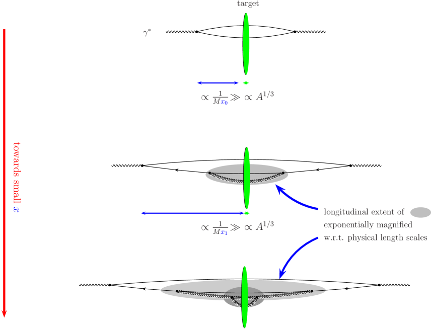
Figure 3: RG corrections to the average over background field configurations. The shaded areas contain the contributions subsumed into the averaging procedure at successive values of $\tau=\ln(1/x)$.

The result of this procedure is the Jalilian-Marian+Iancu+McLerran+Weigert+Leonidov+Kovner equation [13, 14, 15, 16, 18, 21, 22, 23, 24] [the order of names was chosen by Al Mueller to give rise to the acronym JIMWLK, pronounced “gym walk”]. This equation and its limiting cases will be discussed in detail in the next section.

Let us close here with a few phenomenological expectations for the key ingredient of our phenomenological discussion, the dipole cross section. Clearly, we expect the underlying expectation value of the dipole operator,

$$N_{\tau\ \bm{xy}}:=\langle\frac{{\rm tr}(1-U_{\bm{x}}U^{\dagger}_{\bm{y}})}{N_{c}}\rangle_{\tau=\ln(1/x)}$$ (6)

to vanish outside the target, so that the impact parameter integral essentially samples the transverse target size and thus scales roughly with $A^{2/3}$. For central collisions, i.e. deep inside the target we expect the dependence on the dipole size $\bm{r}=\bm{x}-\bm{y}$ to interpolate between zero at small $\bm{r}$ and one at large $\bm{r}$. This is the idea of color transparency. The simplest model to fit this requirement (which should be good where edge effects can be expected to be small, i.e. for large nuclei) would be to parametrize the $\bm{b}$-dependence with a $\theta$-function and have the $\bm{r}$ dependence interpolate between $0$ and $1$ in a way that the transition is characterized by a single scale $Q_{s}$ usually called the saturation scale.

In such a model, the $\bm{b}$ integral will only provide a normalization factor. The idea that the scale in the $\bm{r}$ dependence carries at the same time all the $\tau=\ln(1/x)$-dependence according to

$$N_{\tau\ \bm{xy}}=N((\bm{x}-\bm{y})^{2}Q_{s}(\tau)^{2})$$ (7)

has actually been used by Golec-Biernat and Wüsthoff [25, 26, 27] to provide a new scaling fit of HERA $F_{2}$ data that is remarkably good. This is particularly true in view of the fact that we are precisely not talking about large nuclear targets. A slight generalization of this scaling ansatz has also been used to connect DIS data on nuclei and protons based on the simple idea underlying the McLerran-Venugopalan model that $Q_{s}$ should increase like

$$(Q_{s}^{2})_{A}=(Q_{s}^{2})_{p}\ A^{1/3}$$ (8)

as the additional gluons encountered in additional nucleons on a straight line path through a larger target add in additional color charges that decorrelate eikonal scatterers on shorter and shorter distances. Despite the fact that the data do not really cover $x$- and $Q^{2}$-ranges where such scaling arguments should reliably hold, the agreement is surprisingly good. It would appear that the data available show a remarkable degree of scaling even in cases that are at best at the edge of regions where we would expect the underlying ideas to fully apply.

In the next section will discuss evolution equation and their relation to scaling features as discussed above. As the ideas there were relying on central collisions we will find that the evolution equations lead to such features there. Indeed they turn out not to be valid in very peripheral regions.

2 A short review of the evolution equations

After the qualitative introduction in the previous section, we will simply state the JIMWLK equation and then discuss its key features and limiting cases in order to connect its properties with the phenomenological discussion above. The JIMWLK equation reads

$$\partial_{\tau}\hat{Z}_{\tau}[U]=-\frac{1}{2}i\nabla^{a}_{\bm{x}}\chi^{ab}_{\bm{xy}}i\nabla^{a}_{\bm{y}}Z_{\tau}[U]$$ (9)

and was first cast in this compact form in [22]. Again, $U_{\bm{x}}$ are the Wilson line variables describing the kinematically enhanced degrees of freedom, $\nabla^{a}_{\bm{x}}$ are functional version of the left invariant vector fields (c.f. Lie derivatives) acting on $U_{\bm{y}}$ according to $i\nabla^{a}_{\bm{x}}U_{\bm{y}}=U_{\bm{x}}t^{2}\delta^{(2)}_{\bm{xy}}$ (for more details see [22]) and

$$\chi^{ab}_{\bm{xy}}:=\frac{\alpha_{s}}{\pi^{2}}\int\!\!d^{2}\!z\ K_{\bm{xzy}}\Big{[}(1-\tilde{U}^{\dagger}_{\bm{x}}\tilde{U}_{\bm{z}})(1-\tilde{U}^{\dagger}_{\bm{z}}\tilde{U}_{\bm{y}})\Big{]}^{ab}\hskip 28.45274ptK_{\bm{xzy}}=\frac{(\bm{x}-\bm{z}).(\bm{z}-\bm{y})}{(\bm{x}-\bm{z})^{2}(\bm{z}-\bm{y}^{2})}\ .$$ (10)

[The “$\sim$” indicates the adjoint representation.] $\hat{Z}_{\tau}[U]$ is the “weight functional” that determines correlators $O[U]$ of $U$ fields according to

$$\langle O[U]\rangle_{\tau}:=\int\!\hat{D}[U]O[U]Z_{\tau}[U]$$ (11)

$\hat{D}[U]$ in Eq. (11) is a functional Haar-measure.

Eq. (9) itself is of the form of a (generalized) functional Fokker-Planck equation. In particular the operator on its right hand side,

$$H_{\text{\tiny FP}}:=\frac{1}{2}i\nabla^{a}_{\bm{x}}\,\chi^{ab}_{\bm{xy}}\,i\nabla^{a}_{\bm{y}}$$ (12)

is indeed self adjoint and positive definite and may therefore be called the Fokker-Planck Hamiltonian of the small $x$ evolution.

As a functional equation, Eq. (9) is equivalent to an infinite set of equations for $n$-point correlators of $U$ and $U^{\dagger}$ fields in any representation of $SU(N_{c})$. These will form a coupled hierarchy due to the $U$-dependent nature of $H_{\text{\tiny FP}}$. The evolution equation for a given correlator of $U$-fields is easily obtained by multiplying both sides of Eq. (9) and integrating the result with a functional Haar measure. Using the self-adjoint nature of $H_{\text{\tiny FP}}$ and the fact that the Lie derivatives do not interfere with the Haar measure we immediately obtain

$$\partial_{\tau}\langle O[U]\rangle_{\tau}=\langle(-\frac{1}{2}i\nabla^{a}_{\bm{x}}\chi^{ab}_{\bm{xy}}i\nabla^{a}_{\bm{y}}O[U])\rangle_{\tau}\ .$$ (13)

The only step remaining in the derivation of the evolution equation for $O[U]$ is to evaluate the Lie derivatives as they act on $O[U]$. The nonlinear nature of $H_{\text{\tiny FP}}$ implies that the expectation value on the r.h.s. will contain more $U$ fields than the l.h.s. and thus a new type of correlator of $U$ fields. To determine $\langle O[U]\rangle_{\tau}$ we thus will need also the evolution equation of this new operator in which the same mechanism will couple in still further $U$ fields. Continuing the process we end up with an infinite hierarchy of equations.

As an example for $O[U]$ with immediate phenomenological relevance we consider the two point function of the dipole operator

$$N_{\tau,\bm{x}\,\bm{y}}:=\langle\hat{N}_{\bm{xy}}\rangle_{\tau}\hskip 56.9055pt\hat{N}_{\bm{x}\,\bm{y}}:=\frac{{\rm tr}(1-U_{\bm{x}}^{\dagger}U_{\bm{y}})}{N_{c}}$$ (14)

[Below we will often suppress the explicit $\tau$ dependence.] Eq. (13) immediately leads to

$$\partial_{\tau}\big{\langle}\hat{N}_{\bm{xy}}\big{\rangle}_{\tau}=\frac{\alpha_{s}N_{c}}{2\pi^{2}}\int\!\!d^{2}z\frac{(\bm{x}-\bm{y})^{2}}{(\bm{x}-\bm{z})^{2}(\bm{z}-\bm{y})^{2}}\big{\langle}\hat{N}_{\bm{xx}}+\hat{N}_{\bm{zy}}-\hat{N}_{\bm{xy}}-\hat{N}_{\bm{xz}}\,\hat{N}_{\bm{zy}}\big{\rangle}_{\tau}$$ (15)

Clearly the r.h.s. depends on a 3-point function containing a total of up to 4 $U^{(\dagger)}$ factors, that in general does not factorize into a product of two 2-point correlators (or linear combinations thereof):

$$\big{\langle}\hat{N}_{\bm{xz}}\,\hat{N}_{\bm{zy}}\big{\rangle}_{\tau}\neq\big{\langle}\hat{N}_{\bm{xz}}\big{\rangle}_{\tau}\big{\langle}\hat{N}_{\bm{zy}}\big{\rangle}_{\tau}\ .$$ (16)

To completely specify the evolution of $\langle\hat{N}_{\bm{xy}}\rangle_{\tau}$ we therefore also need to know $\big{\langle}\hat{N}_{\bm{xz}}\,\hat{N}_{\bm{zy}}\big{\rangle}_{\tau}$. The latter, in its evolution equation, will couple to yet higher n-point functions and thus we are faced with one of the infinite hierarchies of evolution equations that are completely encoded in the single functional equation (9).

Because of the fact that Eq. (9) encodes information on the evolution of all possible n-point functions any generic statement that can be derived without reference to a particular correlator is of particular importance. Interestingly enough, and despite its functional nature it allows us to deduce already some of the main features of the evolution process. First of all, Eq. (9) is of Hamiltonian form with a semi-positive-definite Hamiltonian and describes a diffusion process in which $\tau$ plays the rôle of (imaginary) time. From this observation alone, we get very strong statements without any additional work: the eigenmodes of this Hamiltonian, $Z_{n,\tau}[U]$, possesses positive real eigenvalues $\lambda_{n}$ and a generic solution will evolve as a superposition of such modes in the form

$$Z_{\tau}[U]=\sum\limits_{n}a_{n}e^{-\lambda_{n}(\tau-\tau_{0})}Z_{n,\tau_{0}}[U]$$ (17)

where the sum is a formal sum over all modes in the spectrum. If there is an eigenvalue $\lambda_{0}=0$, this will be the only one not damped away exponentially with $e^{-\lambda_{n}\tau}$ at large $\tau$. Indeed $Z_{\tau,\lambda=0}[U]=1$ furnishes such a candidate and it can be argued to be unique [22]. This solution features as a fixed point of the evolution equation and, since all other contributions naturally die away, it is attractive. This remains true although $H_{\text{FP}}$ is scale invariant and the spectrum, labelled by $n$ in the above, is continuous.

At this fixed point, all correlators will be fully determined by what remains in the averaging procedure after $Z_{\tau}[U]\to 1$, namely the Haar measure. This however will average everything to zero unless the transverse locations of the $U_{\bm{x}_{i}}$ factors in the correlator coincide at least pairwise and for each distinct transverse point remaining there is a singlet piece in the decomposition of the $U$ factors into irreducible representations. This immediately implies that all correlation lengths at $\tau=\infty$ vanish: evolution must erase them at $\tau$ grows. What does that mean for our standard example the two point or dipole correlator? As we have discussed, we expect it to interpolate between zero at small separation and one at large separation, with the transition say at a scale $1/Q_{s}(x_{0})$ at some finite $x_{0}$. $1/Q_{s}(x_{0})$ is the correlation length visible in this correlator. As we lower $x$ the correlation length will shrink to zero and we expect the following qualitative trend in its $x$ evolution:

Figure 4: Generic evolution trend for a one scale dipole correlator $N_{\bm{xy}}$ plotted against $|\bm{x}-\bm{y}|$ as $x\to 0$: the curves move towards the left as $\tau=\ln(1/x)$ increases, the asymptotic form being a step function at the origin

There is, in principle, a way to implement Eq. (9) numerically. Eq. (9) is a Fokker-Plank equation and as such can be rewritten as a Langevin equation [22, 28]. The latter can be treated numerically with a lattice discretization of transverse coordinate space. We will discuss this at length in Sec. 3.

It is useful to first study the qualitative properties of this equation in a simplified setting, the only approximation scheme known that preserves the main qualitative features depicted in Figure 4. This turns out to be a $1/N_{c}$ expansion. Viewed from this perspective Eq. (16) turns into

$$\big{\langle}\hat{N}_{\bm{xz}}\,\hat{N}_{\bm{zy}}\big{\rangle}_{\tau}=\big{\langle}\hat{N}_{\bm{xz}}\big{\rangle}_{\tau}\big{\langle}\hat{N}_{\bm{zy}}\big{\rangle}_{\tau}+{\cal O}(\frac{1}{N_{c}})\ .$$ (18)

This is in fact general: dropping the corrections naturally factorizes all $n$-point functions into $2$-point functions and higher correlators decouple for example from Eq. (15). The remainder turns into

$$\partial_{\tau}N_{\bm{xy}}=\frac{\alpha_{s}N_{c}}{2\pi^{2}}\int\!\!d^{2}z\frac{(\bm{x}-\bm{y})^{2}}{(\bm{x}-\bm{z})^{2}(\bm{z}-\bm{y})^{2}}\Big{(}N_{\bm{xx}}+N_{\bm{zy}}-N_{\bm{xy}}-N_{\bm{xz}}\,N_{\bm{zy}}\Big{)}\ ,$$ (19)

where the $\tau$ dependence of the dipole function $N$ is implicitly understood. Eq. (19) was independently derived by Ian Balitsky from his “shock wave formalism” [11, 17] that is completely summarized by Eq. (9) and by Yuri Kovchegov from Mueller’s dipole formalism for the case of large nuclei [20]. Indeed the whole infinite coupled hierarchy of equations represented by Eq. (9) is reduced in content to this one equation for one single function $N_{\bm{zy}}$, called the Balitsky-Kovchegov- or BK-equation.

The main feature of this equation is that it remains consistent with an interpretation of $1-N_{\bm{xy}}$ as a correlator of Wilson lines $\langle{\rm tr}(U^{\dagger}_{\bm{x}}U_{\bm{y}})\rangle/N_{c}$ in that the nonlinearity keeps $N$ between zero and one. Loosely speaking, this is due to a cancellation of the linear and nonlinear terms in $N$ within Eq. (19). In the low density limit, where the $N^{2}$ term is negligible we are left with the BFKL equation in a space time setting as first demonstrated in [17]. The solution for the equation without the nonlinear term is indeed of the BFKL form

$$N_{\tau,\bm{xy}}=\int\frac{d\nu}{2\pi^{2}}d^{2}r_{0}\ ((\bm{x}-\bm{y})^{2})^{-\frac{1}{2}+i\nu}e^{(\tau-\tau_{0})\chi(\nu)}(\bm{r}_{0}^{2})^{-\frac{1}{2}-i\nu}\ N_{\tau_{0},\bm{r}_{0}}$$ (20)

with arbitrary initial condition $N_{\tau_{0},\bm{r}_{0}}$ and $\chi(\nu)$ the BFKL eigenvalue function. This solution is known to grow and spread equally to smaller and larger sizes. The first property limits its range of applicability: as soon as $N$ has grown enough as to “switch on” the nonlinearities, the result Eq. (20) will no longer hold. The second shows that the linear equation spreads into the infrared. Where that happens we have do abandon it altogether. If the nonlinearity is active at short enough distances, i.e. within the perturbative domain we expect two effects: the growth of $N$ should be tamed and the infrared should never affect the evolution.

Numerical studies [29, 30] using a momentum space representation of the BK equation with a boundary condition localized at a single momentum have shown that this is indeed the case. Moreover the solutions have been found to approach a scaling regime in which the coordinate and $x$ dependence are coupled according to

$$N_{\tau,\bm{xy}}=N((\bm{x}-\bm{y})^{2}Q_{s}(x)^{2})\ .$$ (21a)

There the saturation scale $$Q_{s}(x) 1/x$$ grows like a power of . However, the initial conditions and hence the dipole correlators in these simulations do not satisfy the “color transparency” boundary conditions referred to above.

That this simply means that scaling behavior is according to Eq. (21a) is quite generic was shown in [31]. There the authors show that the existence of scaling solutions of the type in Eq. (21a), now with with physics inspired spatial “color transparency” boundary conditions of the type

$$N(0)=0\hskip 28.45274pt\text{and}\hskip 28.45274ptN(\infty)=1\ ,$$ (21b)

also leads to power like growth of the saturations scale according to

$$Q_{s}(x)=\Big{(}\frac{x_{0}}{x}\Big{)}^{\lambda}Q_{0}$$ (22)

If it is possible to satisfy all of the requirements in Eqns. (21), the value of the constant $\lambda$ is determined self-consistently through the equation together with the shape of $N$. That the equation indeed possesses such solutions has, up to now only been demonstrated numerically and form part of our results below. From our simulations it would appear that that single scale initial conditions that satisfy Eq. (21b) typically evolve into scaling solutions of the form Eq. (21a).

In principle it is possible to extend the scaling argument of [31] to solutions of the JIMWLK equation although there one is talking about an infinite hierarchy of different $n$-point functions and the claim that this would naturally fit into a one scale description would sound even more arbitrary than for the BK case. The reason why such solutions are important is that they appear to represent the small $x$ asymptotic behavior for a large class of initial conditions. Unlike the qualitative features imposed by the infinite energy fixed point of Eq. (9), this statement is much more directly amenable to experimental verification: if the initial conditions realized in nature put us not too far from this asymptotic behavior, we find a unique and universal feature in the $x$-dependence of any possible target for which the BK equation yields a reasonable description of the zero impact parameter contributions.

It remains important to understand the conditions under which such behavior can be expected:

First note, that the scaling behavior Eq. (21) with growing saturation scale $Q_{s}$ is just a special case of the generic behavior shown in Fig. 4. Whether we are in a purely one scale situation or in a setting with more than one scale enters the scale that controls the transition of $N_{\tau,\bm{xy}}\to 1$ at large $\bm{r}=\bm{x}-\bm{y}$ sets the infrared scale in the problem as $N$ will not grow beyond $1$. For this to happen we need large densities of gluons. Where this is guaranteed at some initial $\tau_{0}=\ln(1/x_{0})$, general fixed point considerations and explicit simulations show that the IR scales will only get larger as we continue to evolve towards smaller $x$. Where the initial IR scale is not perturbative the derivation of the evolution equations is not valid, however. This limits our description to central impact parameters off large enough nuclei.

Besides these facts there remains a lot to be learned about solutions to the nonlinear evolution equations presented in this section. This is the goal of this paper.

Obviously, the main advantage of Eq. (19) over the Langevin representation of Eq. (9) is its simplicity. Although, even here, no analytical solutions are available, the numerical task at hand is much more tractable. If we can establish that this equation allows us to identify most of the qualitative features of the full evolution, we can use it to explore the main features of small $x$-evolution an only then resort to a numerical treatment of Eq. (9) in the most interesting regions to get quantitatively precise results. It is precisely this rôle in which we are going to utilize the BK-equation.

Our work consists of two main parts:

• First, we perform a study of the JIMWLK equation, using its Langevin form implemented using a lattice discretization of transverse space.

  This is the first coordinate space treatment of either the JIMWLK or BK equations and we are the first to show directly that the solutions approach the fixed point as qualitatively predicted in [22], c.f. Fig. 4.

  At the same time we will be able to confirm IR safety of the JIMWLK equation via numerical simulations.

  Still at finite $\tau$ we will see that scaling solutions emerge that are characterized by a saturation scale $Q_{s}(x)$, a feature already found earlier in the context of the BK-equation [30, 29].

  The initial conditions chosen in this study are almost free of any $N_{c}$-violations. We measure how these fare under full JIMWLK evolution and find that the equations appear to neither enhance nor dampen the extent of these.

  To complement our study of IR stability we also carefully study the UV or continuum limit. We will show that diffusion into the UV is not tamed. Recalling the properties of the BFKL equation this does not come as a complete surprise. However, we will show that for some quantities like the evolution rate $\lambda_{\tau}:=\partial_{\tau}\ln(Q_{s}(\tau))$ this fact makes a reliable continuum extrapolation based on JIMWLK a task of enormous computational cost.

  Due to the nearly perfect $N_{c}$-factorization properties associated with the initial conditions used we are then able to complement our JIMWLK studies with BK simulations implemented with same type of lattice UV regulator. This allows for a more thorough study of the continuum limit and reveals even closer agreement of JIMWLK and BK behavior for the classes of initial condition chosen. We will show that the active phase space in both cases extends to up to 7 orders of magnitude above $Q_{s}$, the physical scale of the problem. In such situations one is typically forced to resum large logarithmic corrections to get quantitatively reliable results. This then leads us to the second part:

• Motivated by results found in connection with the BFKL equation we will identify left out running coupling effects as the main culprits for the largeness of UV phase space. We perform simulations with a coupling running with the size of the parent dipole as $\alpha_{s}(1/(\bm{x}-\bm{y})^{2})$ and establish that this removes the extraneous phase space and thus resums large phase space corrections. Only with this resummation in place the main contributions to evolution originate at distances at and around $1/Q_{s}(x)$ and the coupling indeed is of the order of $\alpha_{s}(Q_{s}(x)^{2})$ as anticipated in the underlying physics picture.

  $\Lambda_{\text{QCD}}$ and scale breaking enter our simulation as a consequence of this step. This, at least conceptually, breaks the asymptotic, geometric scaling limit of the equations. Numerical evidence nevertheless shows that the solutions still converge to an approximate asymptotic form that shows almost perfect geometric scaling, in agreement with [32]. Nevertheless we will show that a clear modification of the $x$-dependence of $Q_{s}$ emerges, away from the simple fixed coupling $(x_{0}/x)^{\lambda}$-form. $\lambda_{\text{eff}}$ (suitably defined, see below) picks up pronounced $\tau$ dependence and the numerical values change drastically: we find typically a factor of two to three compared to the fixed coupling situation. While the necessity of the inclusion of running coupling effects had been seen already in estimates of evolution rates and numerical simulations [29, 32] as well as phenomenological fits of HERA data [33], size and conceptual importance of these corrections has not been discussed from the viewpoint taken here.

3 JIMWLK and BK equations at fixed coupling

3.1 Simulating the JIMWLK equation

To be able to solve the JIMWLK equation directly we need a numerical method to implement its content. Such a method offers itself after translating the Fokker-Planck equation to a Langevin equation. Such an approach has already been suggested in [22] and a derivation has been given in [28] where we refer the reader for details. For the interested, we provide a short exposition of the key steps of a derivation that highlights the close connection between Langevin equations and path-integrals in App. A.

To prepare translation into Langevin form we follow [22] and write the RG again in standard form

$$\frac{\partial}{\partial\tau}\hat{Z}[U] =-\nabla^{a}_{\bm{x}}\Big{[}\frac{1}{2}\nabla^{b}_{\bm{y}}\hat{\chi}^{ab}_{\bm{xy}}-\big{(}\frac{1}{2}\nabla^{b}_{\bm{y}}\hat{\chi}^{ab}_{\bm{xy}}\big{)}\Big{]}\hat{Z}[U]$$ (23)

and define

$$\hat{\sigma}^{a}_{\bm{x}}:=\frac{1}{2}\nabla^{b}_{\bm{y}}\hat{\chi}^{ab}_{\bm{xy}}=-i\big{(}\frac{1}{2}\frac{\alpha_{s}}{\pi^{2}}\int\!\!d^{2}z\frac{1}{({\bm{x}}-{\bm{z}})^{2}}\tilde{\rm tr}(\tilde{t}^{a}\tilde{U}_{\bm{x}}^{\dagger}\tilde{U}_{\bm{z}})\Big{)}$$ (24)

(the “$\sim$” indicating adjoint matrices and traces).

We then abandon the description in terms of weight functionals $\hat{Z}_{\tau}$ in favor of one in terms of ensembles of fields which are governed by the corresponding Langevin equations.

Explicitly, to calculate any observable $O[U]$ of the fields $U$ we write

$$\langle O[U]\rangle_{\tau}=\int\!\hat{D}[U]O[U]\hat{Z}_{\tau}[U]\approx\frac{1}{N}\sum\limits_{U\in{\sf E}[\hat{Z}_{\tau}]}O[U]$$ (25)

where, separately at each $\tau$, the sum is over an ensemble ${\sf E}[\hat{Z}_{\tau}]$ of $N$ configurations $U$ whose members were created randomly according to the distribution $\hat{Z}_{\tau}$. Clearly, for $N\rightarrow\infty$, the ensemble and $\hat{Z}_{\tau}$ contain the same information.

The Langevin equation then schematically reads

$$\partial_{\tau}\,[U_{\bm{x}}]_{ij}=[U_{\bm{x}}it^{a}]_{ij}\Big{[}\int\!\!d^{2}y\,[{\cal E}_{\bm{x}\bm{y}}^{ab}]_{k}[\xi^{b}_{\bm{y}}]_{k}+\hat{\sigma}^{a}_{\bm{x}}\Big{]}$$ (26)

where

$${\cal E}^{ab}_{{\bm{x}}{\bm{y}}}=\left(\frac{\alpha_{s}}{\pi^{2}}\right)^{1/2}\frac{({\bm{x}}-{\bm{y}})_{k}}{({\bm{x}}-{\bm{y}})^{2}}[1-\tilde{U}^{\dagger}_{\bm{x}}\tilde{U}_{\bm{y}}]^{ab}$$ (27)

is the “square root” of $\chi$, $\chi^{ab}_{{\bm{x}}{\bm{y}}}={\cal E}^{ac}_{{\bm{x}}{\bm{z}}}{\cal E}^{cb}_{{\bm{z}}{\bm{y}}}$, and $\xi$ are independent Gaussian random variables with correlators determined according to

$$\langle\ldots\rangle_{\xi}=\int\!D[\xi]\,(\ldots)\,e^{-\frac{1}{2}\xi\xi}\ .$$ (28)

Note the factor of $i$ which is essential to render this an equation for an infinitesimal change of an element of $SU(N_{c})$. In fact the components of $\omega^{a}_{\bm{x}}:=\Big{[}\int\!\!d^{2}y\,[{\cal E}_{\bm{x}\bm{y}}^{ab}]_{k}[\xi^{b}_{\bm{y}}]_{k}+\hat{\sigma}^{a}_{\bm{x}}\Big{]}$ can be directly interpreted as the “angles” parametrizing a local gauge transformation in transverse space.

It is of particular importance to note that the possibility to formulate the stochastic term via a completely decorrelated Gaussian noise $\xi$, that is to say with $\langle\xi^{a,i}_{\bm{x}}\xi^{b,j}_{\bm{y}}\rangle=\delta^{ab}\delta^{ij}\delta^{(2)}_{\bm{x}\bm{y}}$, reduces the numerical cost for a simulation like this considerably.

In our practical implementation, we discretize the Langevin equation in Eq. (26) using a regular square lattice of $N^{2}$ sites (volume $(Na)^{2}$, where $a$ is the lattice spacing), with periodic boundary conditions. In dimensionless units ($a=1$) and defining a rescaled, discrete, evolution time

$$s:=\frac{\alpha_{s}}{\pi^{2}}\tau$$ (29)

the Langevin equation becomes

$$U({\bm{x}};s+\delta s)=U({\bm{x}};s)\exp[it^{a}\omega^{a}({\bm{x}};s)]$$ (30)

where

$$\omega^{a}({\bm{x}},s) = \sqrt{\delta s}\sum_{{\bm{y}}}K_{i}({\bm{x}}-{\bm{y}})[1-\tilde{U}^{\dagger}({\bm{x}};s)\tilde{U}({\bm{y}};s)]^{ab}\xi_{i}^{b}({\bm{y}})$$ (31)

$$- \delta s\sum_{{\bm{y}}}S({\bm{x}}-{\bm{y}})\frac{1}{2}\tilde{\rm tr}[i\tilde{t}^{a}\tilde{U}^{\dagger}({\bm{x}},s)\tilde{U}({\bm{y}},s)].$$

Here

$$K_{i}({\bm{r}})=\frac{{\bm{r}}_{i}}{{\bm{r}}^{2}}\,,\hskip 56.9055ptS({\bm{r}})=\frac{1}{{\bm{r}}^{2}},$$ (32)

and $\xi$ is a Gaussian noise with $\langle\xi_{i}^{a}({\bm{x}})\xi_{j}^{b}({\bm{y}})\rangle=\delta_{ij}\delta^{ab}\delta_{{\bm{x}},{\bm{y}}}.$ $K_{i}({\bm{r}})$ and $S({\bm{r}})$ are taken to be $=0$ if ${\bm{r}}=0$.

In practical numerical work we have to carefully consider the following issues:

Boundary conditions:  The sum over the volume (${\bm{y}}$) above must be defined in conjunction with the boundary conditions used. In general, the periodic boundary conditions minimize the effects of the finite volume and makes the system, on average, translationally invariant. Because of the long range of the evolution kernel the distance between points ${\bm{x}}$ and ${\bm{y}}$ must be evaluated taking the periodicity into account. This can be done in several non-equivalent ways; we choose one which evaluates the distance $({\bm{x}}-{\bm{y}})$ to be the shortest one while taking the periodicity into account. This is achieved by modifying the argument of the functions $K_{i}$ and $S$ as follows:

$$({\bm{x}}-{\bm{y}})\mapsto({\bm{x}}-{\bm{y}})+\bm{n}N,$$ (33)

where $n_{i}\in\{-1,0,1\}$ is chosen to minimize the absolute value of the r.h.s. of Eq. (33). This procedure cuts the range of the evolution kernel to be $\leq N/2$, i.e. we take the volume integral over a single periodic copy of the volume.

Let us note here that the boundary condition is significant only if the saturation radius $R_{s}\sim 1/Q_{s}$ is of order system size. As we shall see below, the boundary conditions (or the system size) have a negligible effect on the evolution as long as $1/Q_{s}\ll N$.

Fourier acceleration:   Due to the non-locality of the evolution operator, one time step evolution of the $N\times N$ system using Eq. (31) requires $\propto N^{4}$ numerical operations. This is impractical except for the smallest volumes. However, we note that Eq. (31) can be decomposed into convolutions as follows:

$$\omega^{a}=\sqrt{\delta s}\left[C(K_{i},\xi_{i}^{a})-(\tilde{U}^{\dagger})^{ab}C(K_{i},\tilde{U}^{ab}\xi^{b}_{i})\right]-(\delta s)\left[(t^{a})^{bc}(\tilde{U}^{\dagger})^{cd}C(S,\tilde{U}^{db})\right].$$ (34)

The convolution can be evaluated with Fourier transformation:

$$C(A,B)_{{\bm{x}}}=\sum_{{\bm{y}}}A({\bm{x}}-{\bm{y}})B({\bm{y}})={\cal F}^{-1}[{\cal F}(A){\cal F}(B)].$$ (35)

Thus, using FFTs the cost can be reduced to $N^{2}\log N$, which makes a huge difference. Nevertheless, the cost is still large: there are 192 normal or inverse transformations in each time step (note that $K_{i}$ and $S$ need to be transformed just once).

Time discretization:  The discrete time step $(\delta s)$ introduces an error $\propto(\delta s)^{2}$ for each update step. We chose $\delta s$ so that the largest values of $\omega^{a}({\bm{x}})$, which characterizes the change in $U({\bm{x}})$ in a single step, always remains smaller than $0.3$. This resulted to time steps $\delta s\sim 5\times 10^{-5}$, which is overly conservative; even quadrupling $\delta s$ had no observable effect on the evolution.

Spatial continuum limit:  It is essential to have control over the finite lattice cutoff effects. In the continuum the evolution equations are completely scale invariant; the physical length scale is given by the initial conditions. On the lattice we have 2 new scales, lattice size $L$ and -spacing $a$ (which equals 1 in dimensionless units above). These scales must be chosen so that the physical scale, saturation scale $R_{s}$, is safely between them; in any case, the effects of the finite IR and UV cutoffs must be checked. In short, it turns out that the requirement $R_{s}\ll L$ is easy to satisfy; a factor of 3–4 is sufficient in order to have a negligible effect (i.e. there are no IR problems). On the other hand, we find that $a$ should be several orders of magnitude smaller than $R_{s}$ for the UV effects to vanish, making the continuum limit very non-trivial.

Initial conditions:  For the initial condition we choose a distribution of $U$-matrices with a Gaussian correlation function:

$$\langle U^{\dagger}_{\bm{x}}U_{\bm{y}}\rangle\propto\exp\left(\frac{-({\bm{x}}-{\bm{y}})^{2}}{4R^{2}}\right).$$ (36)

Scale $R$ here is close to the initial saturation scale $R_{s}$ (depending on the precise definition of $R_{s}$).

For a linear (scalar or vector) field it is straightforward to generate distributions with (almost) arbitrary initial 2-point correlation functions, $\langle A_{0}A_{\bm{x}}\rangle=C_{\bm{x}}$, using Fourier transformations: just let $A_{\bm{k}}\propto\sqrt{C_{\bm{k}}}\xi_{\bm{k}}$, where $\xi_{\bm{k}}$ is white Gaussian noise, $P(\xi)\propto\exp(-\xi^{2})$, and $C_{\bm{k}}$ is Fourier transform of $C_{{\bm{x}}}$. Field $A_{\bm{x}}$ is obtained with an inverse Fourier transformation.

In our case the degrees of freedom are elements of SU(3) group and this method cannot be applied directly. However, we can utilize the approximate linearity of small changes in group elements and build up the desired distributions in short steps. The method works as follows: let the desired correlation function be $\langle U^{\dagger}_{\bm{x}}U_{0}\rangle=C_{\bm{x}}$. We start from initial state $U_{\bm{x}}=1$ and repeat the operation

$$U_{\bm{x}}\leftarrow e^{iA_{\bm{x}}/\sqrt{n}}U_{\bm{x}}$$ (37)

$n$ times, generating new suitably distributed adjoint matrices $A_{\bm{x}}=A_{\bm{x}}^{a}t^{a}$ for each step. Here $A^{a}_{\bm{x}}$ is a Fourier transform of $A^{a}_{\bm{k}}\propto(C^{A}_{\bm{k}})^{1/2}\xi^{a}_{\bm{k}}$, where $\xi^{a}_{\bm{k}}$ are independent Gaussian random variables and $C^{A}_{\bm{k}}$ is the Fourier transform of $-\ln C_{\bm{x}}$ (The use of the logarithm is a trick to give the correct asymptotics to the correlation function.).

Thus, the matrices $U_{\bm{x}}$ “diffuse” towards the desired state by random walking along the group manifold. The number of the steps, $n$, has to be large enough in order to give us properly randomized $U$-matrices. Naturally, the method is only approximate, but the deviations from the desired correlation function remain small.

We also used another, completely unrelated, method for generating the initial state: this time we start from a completely random configuration of $U_{\bm{x}}$-matrices $\in$ SU(3), and make the substitution

$$U_{\bm{x}}\leftarrow\exp(\frac{1}{2}R^{2}\nabla^{2})U_{\bm{x}}\approx(1+\frac{1}{2n}R^{2}\nabla^{2})^{n}U_{\bm{x}}\,,$$ (38)

for $n$ large enough. $\nabla^{2}$ is evaluated as lattice finite differences. Thus, the last expression tells us to “smear” the matrix $U_{\bm{x}}$ with its neighbors $n$ times. For linear fields this procedure yields exactly Gaussian 2-point function $\langle U_{\bm{x}}U_{b}y\rangle\propto\exp[-({\bm{x}}-{\bm{y}})^{2}/2R^{2}]$. This is straightforward to verify by making a Fourier transformation of Eq. (38). However, because we have to ensure that $U_{\bm{x}}$ remains on the group manifold, we have to project $U$ back to SU(3) after each step. This is done by finding $U^{\prime}\in\mbox{SU(3)}$ which maximizes ${\rm tr}(U^{\dagger}U^{\prime})$, and substituting $U\leftarrow U^{\prime}$. The projection step makes the initial state generation method again approximate.

Both of these two methods yield initial ensembles which have almost Gaussian initial 2-point functions. Due to performance reasons we used mostly the first method (the latter method requires $n\gg L$ in order to really produce long-distance correlations).

3.2 Numerical results from JIMWLK simulations

In our analysis we use volumes $30^{2}$–$512^{2}$, with 8–20 independent trajectories (with independent initial conditions) for each volume. This amount of statistics proved to be sufficient for our purposes; actually trajectory-by-trajectory fluctuations in the dipole operators are quite small (i.e. already one trajectory gives a good estimate of the final result).

In Fig. 5 we show the evolution of the dipole operator, averaged over 8 independent trajectories on a $256^{2}$ lattice, from interval $\alpha_{s}\tau\equiv\alpha_{s}\ln(1/x)=0\ldots 2.5$. Qualitatively, we can observe that the dipole operator soon approaches a specific functional scaling form, where the shape is preserved but the length scale is shortened under the evolution. This is clearly visible on the logarithmic scale plot on the right: the Gaussian initial condition quickly settles towards the scaling solution which evolves by moving towards left while approximately preserving the shape.

Figure 5: Evolution of the dipole operator from the JIMWLK equation on an $256^{2}$ lattice, shown on a linear (left) and logarithmic (right) distance scale. The general pattern as predicted from the existence of the fixed point and drawn qualitatively in Fig. 4 shows up clearly. On the right we see a scaling form emerge: a stable shape of the curve that merely shifts to the left unaltered.

From the dipole correlation function we can now measure the evolution of the saturation length scale $R_{s}$. There are several inequivalent ways to measure $R_{s}$ from the dipole function; perhaps the most straightforward and robust method is to measure the distance where the dipole function reaches some specified value. This is the approach we adopt here; precisely, we define $R_{s}(\tau)$ to be the distance where the dipole function $N((\bm{x}-\bm{y})^{2})=1/N_{c}{\rm tr}\langle 1-U^{\dagger}_{\bm{x}}U_{\bm{y}}\rangle$ reaches a value $c$:

$$N(R_{s}^{2}):=c$$ (39)

where $c$ should not be much smaller than 1. The precise definition of course is $c$-dependent – different choices will lead to a rescaling of the value of $R_{s}$ – and we adopt the convention to set $c=1/2$. Such a definition can be used both inside and outside the scaling region and will encode some physics information in both.

In Fig. 7 we show $R_{s}(\tau)$, measured from various lattice sizes and initial values for $R_{s}(\tau=\tau_{0})$. Since the initial $\tau_{0}$ is not a physical observable in the sense that we are not in position to match initial conditions to experiment, we are at liberty to shift the $\tau$-axis for each of the curves in order to match the curves together. In Fig. 7 this procedure clearly gives us a section of the $R(\tau)$ curve, independent of the system size or initial size.

From $R_{s}(\tau)$ we obtain the instantaneous evolution speed

$$\lambda=-\frac{\partial\ln R_{s}}{\partial\tau}.$$ (40)

Note that contrary to $R_{s}$ this quantity is unique and independent of the convention for $c$ in Eq. (39) inside the scaling regime. Outside this uniqueness is lost.

In Fig. 7 we show $\lambda$ plotted against $R_{s}$, measured from several volumes and initial sizes. The curves naturally evolve from right to left, from large $R_{s}$ towards smaller values. As opposed to Fig. 7, in this case the curves are fully determined by the measurements. Note that for a scale invariant evolution $\lambda$ should be constant, independent of $R_{s}$. This is clearly not the case here. We observe the following features:

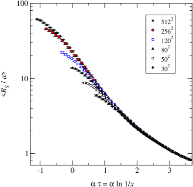
Figure 6: The evolution of the saturation scale $R_{s}$, measured from system sizes $30^{2}$ – $512^{2}$. The curves are shifted in $\tau$ to match at large $\tau$.

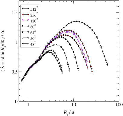
Figure 7: The evolution speed $\lambda=-\partial_{\tau}\ln R_{s}$ plotted against $R_{s}$ for various system sizes and initial $R_{s}$.

• $\lambda$ starts relatively small but increases rapidly. We interpret this to be due to the settling of the Gaussian initial state towards the scaling form. This change in shape is clearly visible in Fig. 4. Such behavior typical for initial state effects. This effect should be much smaller if the initial ensemble would more closely resemble the scaling solution. In these particular simulations, in which we were mainly interested in universal features of the evolution equations at larger $\tau$, part of the initial changes also arise from the fact that the initial $R_{s}$ may be too large; i.e. the initial state dipole function may be too far away from unity at distances $L/2$, the maximum distance on a $L^{2}$ lattice.

• At small $R_{s}$ (large $\tau$), $\lambda(R_{s})$ clearly settles on an universal curve, which decreases with decreasing $R_{s}$. This curve is a function of $R_{s}/a$, i.e. the saturation scale in units of the lattice spacing. Thus, this is a UV cutoff effect which should vanish (curve turn horizontal) when $a\rightarrow 0$ ($R_{s}/a\rightarrow\infty$). However, we are clearly still far from this case, even on largest volumes. In order to obtain a continuum limit, one should perform extrapolation $a\rightarrow 0$. We do this as follows: first, we note that the maxima of $\lambda(R_{s}/a)$ -curves for each of the runs fall on a universal curve when plotted against $a/R_{s}$ at maximum. This is shown in Fig. 9. Linear function does not fit the data well; on the other hand, fitting a power law + constant we get a reasonable match (shown in the figure). However, with the steepest part of the curve in a region without data it is clear that the extrapolation is not safe. Without a definite functional form for the extrapolation our data is not good enough to allow for a reliable continuum limit estimate. (Nevertheless, we note that the comparison to BK simulation results, discussed below, makes the continuum limit in JIMWLK much clearer.)

• On the other hand, the IR cutoff effects appear to be mild: the behavior of $\lambda(R_{s})$ curves is largely determined by the initial radius $R_{s}(\tau_{0})$, independent of the system size $L$ (so far as $L$ is clearly larger than $R_{s}$). This is clarified in Fig. 9, where evolution of $R_{s}(\tau)$ is shown from volumes $30^{2}$ – $64^{2}$, using the same $R_{s}(\tau_{0})\approx 6a$. Only small initial deviations are seen.

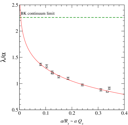
Figure 8: Approach to the continuum limit of $\lambda/\alpha$ against $a$ in units of $R_{s}$. The values are taken from the maxima in Fig. 7. The dashed line on the top shows the continuum value obtained from a simulation of the BK equation. A continuum extrapolation (continuous line) from this alone appears unreliable with most of the data away from the steep section.

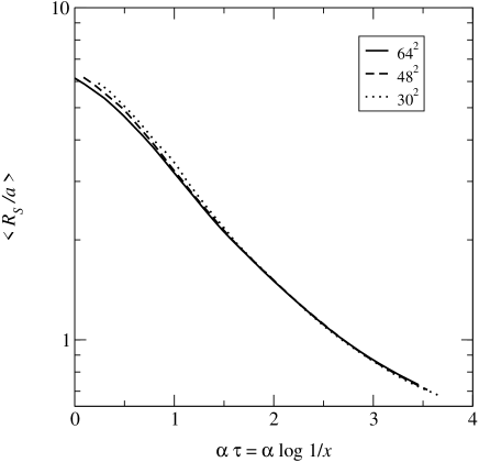
Figure 9: The evolution of the saturation scale with different IR cutoffs (lattice sizes). Except for a small initial difference, the differences are well within statistical errors.

Thus, the necessity of having a very large hierarchy of the relevant scales $a\ll R_{s}<L$ prevents us from making continuum extrapolations. The cutoff sensitivity problem is also present in the BK equation (19). However, the BK equation is much simpler to study numerically than the full JIMWLK equation: firstly, there is only a single degree of freedom, a scalar field instead of a SU(3) matrix field, and secondly the evolution equation is fully deterministic, instead of statistical. This enables us to study much larger range of volumes and initial conditions with reduced errors.

Moreover, under certain conditions, the BK equation can be expected to be a fairly good approximation of the JIMWLK equation: in Fig. 10 we show the difference of 4-field correlators

$$\langle{\rm tr}(U_{\bm{x}}^{\dagger}U_{\bm{y}}){\rm tr}(U_{\bm{y}}^{\dagger}U_{\bm{z}})\rangle-\langle{\rm tr}(U_{\bm{x}}^{\dagger}U_{\bm{y}})\rangle\langle{\rm tr}(U_{\bm{y}}^{\dagger}U_{\bm{z}})\rangle.$$ (41)

For concreteness, we chose the points so that $({\bm{x}}-{\bm{y}})\parallel\bm{e}_{1}$, $({\bm{y}}-{\bm{z}})\parallel\bm{e}_{2}$ and $|{\bm{x}}-{\bm{y}}|=|{\bm{y}}-{\bm{z}}|$. The natural magnitude for these correlators is $\sim 1$. Thus, given the initial conditions we used, we see that the correlators cancel to a 1–2 % accuracy, with the violations staying roughly at the same size throughout the $\tau$ interval covered.

Figure 10: Factorization violation for a $4$-field correlator. Typical error size is indicated by dashed lines for a curve in the middle. They are generically small and indicate that the large $N_{c}$ limit, i.e. the BK equation will be a good approximation as long as the initial condition does not contain strong $1/N_{c}$ corrections.

This seems to indicate that for the type of initial conditions used, the BK equation should give a good approximation of the salient features of the evolution. In particular we should be able to refine our understanding of the UV extrapolation and augment Fig. 9 with results from BK simulations in which we also use a lattice representation for transverse space to parallel our treatment of the JIMWLK equation.

3.3 BK and JIMWLK compared

In order to study the cutoff-dependence and to facilitate the comparison with JIMWLK simulations we study the BK equation with two different numerical approaches.

First, we discretize Eq. (19) on a regular square lattice with periodic boundary conditions as in JIMWLK. Using the translation invariance, we can substitute $N_{{\bm{x}}{\bm{y}}}\rightarrow N_{{\bm{x}}-{\bm{y}}}$, and set, for example, ${\bm{y}}=0$ in Eq. (19), obtaining

$$\partial_{\tau}N_{\bm{x}}=\frac{\alpha_{s}N_{c}}{2\pi^{2}}\int\!\!d^{2}z\frac{{\bm{x}}^{2}}{({\bm{x}}-{\bm{z}})^{2}{\bm{z}}^{2}}\Big{(}N_{{\bm{x}}-{\bm{z}}}+N_{\bm{z}}-N_{\bm{x}}-N_{{\bm{x}}-{\bm{z}}}\,N_{\bm{z}}\Big{)}\ .$$ (42)

This equation can be readily simulated on a square lattice. The evolution kernel again can be written in terms of convolutions, and can be efficiently evaluated using FFTs. We again make the choice that when ${\bm{z}}=0$ or ${\bm{z}}={\bm{x}}$, the integral kernel evaluates to zero. The periodicity is taken into account analogously to the JIMWLK equation.

The second method we use has been developed by [29], similar results had earlier been obtained in [30]. By first Fourier transforming the evolution equation (19) to momentum space, it can be further transformed into a form which depends only on logarithmic momentum variable $\xi\sim\ln k^{2}$. In this form the kernel involves only 1-dimensional integral, and it becomes easy to include a very large range of momenta in the calculation; in our case, more than 20 orders of magnitude. Thus, this enables us to obtain a cutoff-independent continuum limit result for the evolution exponent $\lambda$. The key result we obtained with this method was already shown in Fig. 9 for comparison with the JIMWLK extrapolation.

Figure 11: The evolution of $N({\bm{r}})$ on a $4096^{2}$ lattice, measured along on-axis direction. The curves are plotted with interval $\delta\tau=0.25/\alpha$, and the total evolution time is $7/\alpha$.

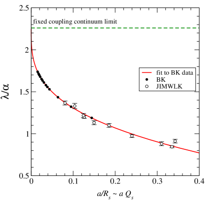
Figure 12: Continuum extrapolations for $\lambda$ using JIMWLK and BK simulations. The UV cutoff is plotted in units of the physical scale $R_{s}$. The continuous line is $\lambda/\alpha_{s}=2.26-2.0(a/R_{s})^{0.32}$

In Fig. 12 we show the evolution of $N$ measured from $4096^{2}$ lattice. The similarity with the dipole function of JIMWLK equation is striking, see Fig. 5. Again we see the initial settling towards the scaling form, which evolves by shifting towards smaller $R$ while preserving the shape. Also here we see that, even with a scaling form reached, the spacing of curves and hence $\lambda$ is not constant. This again is due to the growing influence of the UV cutoff.

We are now in a position to complement our results from the JIMWLK equation. We extract $\lambda$ in the same way as in Figs. 7 and 9. This time, there are no statistical errors in the measurements of $\lambda$. A function of form $\lambda/\alpha_{s}=c_{1}+c_{2}(a/R_{s})^{\nu}$ is an excellent fit to the data, with result $c_{1}=2.26$, $c_{2}=2.0$ and $\nu=0.32$. The $a\rightarrow 0$ result agrees perfectly with the momentum space result. This is shown in Fig. 12. The agreement of BK and JIMWLK results at corresponding cutoff scales is remarkable over the whole range. Most striking is an evaluation of the active phase space. While on the IR side activity is limited to within one order of magnitude of the saturation scale $Q_{s}$, on the UV side we need the cutoff about 6 orders of magnitude larger than $Q_{s}$ to get within 1% of the continuum value.as is easily extracted from the power law fit.

This situation is clearly unnatural: large open phase space of this magnitude usually generates large logarithmic corrections that need to be resummed to get physically reliable results. In the following we will argue that the main source for such corrections are due to running coupling and study the effects which, among other new qualitative features, will bring a large reduction of active phase space in the context of the BK equation that erases the potential for large logarithmic corrections.

4 Running coupling effects

To account for running coupling effects in the simplest possible way, we decide to have the coupling run at the natural scale present in the BK-equation, the size of the parent dipole $(\bm{x}-\bm{y})^{2}$, i.e. in Eq. (19), we replace the constant $\alpha_{s}$ by the one loop running coupling at the scale $1/(\bm{x}-\bm{y})^{2}$:

$$\alpha_{s}\to\alpha_{s}(1/(\bm{x}-\bm{y})^{2})=\frac{4\pi}{\beta_{0}\ln\frac{1}{(\bm{x}-\bm{y})^{2}\Lambda^{2}}}\hskip 28.45274pt\text{with}\hskip 28.45274pt\beta_{0}=(11N_{c}-2N_{f})/3$$ (43)

$\Lambda$ in Eq. (43) is related to $\Lambda_{\text{QCD}}$ by a simple factor of the order of $2\pi$. Such a simple replacement, of course, is not what we expect to arise from an exact calculation in which the two loop contributions that generate the running will emerge underneath the integral over $\bm{z}$. This comes on top of the fact that at next to leading order there will be corrections beyond the running coupling effects that are entirely unaccounted for by this substitution. Nevertheless, we would like to argue that Eq. (43), when used in the BK equation captures the leading effect associated with the “extraneous” phase space uncovered in Sec. 3.3. This has been the outcome of a long discussion in the context of the BFKL equation and its next to leading order corrections [34, 35, 36, 37, 38, 39, 40] Here we simply take this as our starting point with the attitude that a scale setting technique like the one employed in Eq. (43) is but the easiest way to get even quantitatively reliable initial results. We plan on supplementing this with more detailed studies based on dispersive methods of implementing the running coupling effects.

With running coupling we have to face the presence of the Landau pole in Eq. (43). The main point here is, that while indeed we do not control what is happening at that scale we are justified in providing a prescription for its treatment. With $Q_{s}\gg\Lambda_{\text{QCD}}$ the integral on the r.h.s. of the BK equation yields extremely small contributions at scales of the order of $\Lambda_{\text{QCD}}$, typically of the order of $10^{-7}$ times what we see around $Q_{s}$. This is the reason why we are allowed to ignore whatever happens there and to freeze any correlators such as $N$ at these scales at the values provided by the initial condition – a reasoning that is already necessary at fixed coupling in some sense. If we turn on running coupling then, the physical thing to do is to switch off the influence of the divergence at the Landau pole, for instance by freezing the coupling below some scale $\mu_{0}$. Of course we make sure that the details of where we do that will not affect our results.

Such an argument about the integrals on the r.h.s. is valid at $b\approx 0$ or infinite transverse target size where the nonlinearity is present and sizable everywhere we look. For large $b$ one necessarily enters the region where the nonlinearity is small and there one would remain sensitive to any value of $\mu_{0}$. That is our reason for not considering such situations.

Let us now explore how this modification affects evolution. The crucial first observation is a clear reduction of active phase space as shown in Fig. 13: on the left panel we show an example for the extrapolation of $\lambda/\alpha_{s}(Q_{s}(\tau)^{2})$ to its continuum value at one value of $\tau$ (corresponding to $\alpha_{s}(Q_{s}(\tau)^{2})=0.2$) and compare to the fixed coupling case.

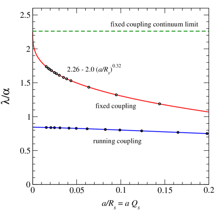
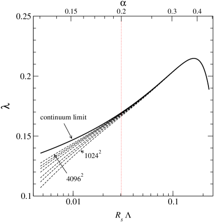
Figure 13: Left: example of a continuum extrapolation of $\lambda/\alpha_{s}(Q_{s}(\tau)^{2})$ for a fixed initial condition at a $\tau$-value where $\alpha_{s}(Q_{s}(\tau)^{2})=0.2$, compared to the fixed coupling case. Right: $\lambda(R_{s}(\tau))$, measured using different lattice cutoffs, together with the extrapolated continuum limit curve. The dashed vertical line indicates the point where the values on the left are extracted.

With running coupling we are able to reach the continuum limit already for relatively small lattices, i.e. with a UV cutoff that would be orders of magnitude too small in the corresponding fixed coupling run. Note that as a consequence the continuum value is reduced by a noticeable factor. On the right panel we demonstrate how the extrapolation was done: for a given initial condition we perform runs with different lattice spacings and measure $\lambda(\tau)$ and $R_{s}(\tau)$. We get a reliable continuum limit extrapolation for $\lambda$ in a wide range of $\tau$-values; when $R_{s}$ becomes small ($\sim 5$–$10a$) the measurements start to fan out. However, as will be shown in Fig. 16, we can extend the measurements by starting from different initial $R_{s}$-values.

We will turn to a more systematic study below and only emphasize that the results given in what follows are physical in the sense that they apply to the continuum limit.

First and foremost, the running coupling reflects the breaking of scale invariance. It would be natural to expect that the dipole function now might never exhibit the scaling behavior of Eq. (21a) that was so characteristic at large $\tau$ for fixed coupling. In fact numerical evidence suggests otherwise. As shown in Fig. 15 which shows results $N_{\tau,\bm{xy}}$ for large $\tau$ against $r\,Q_{s}(\tau)$. The different curves only slightly deviate from each other: scaling is only violated very weakly. We attribute this to the fact that $Q_{s}(\tau)\gg\Lambda_{\text{QCD}}$ and thus the scale breaking is not strongly communicated to the active modes.

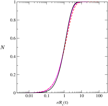
Figure 14: Approximate scaling behavior of $N_{\tau,\bm{xy}}$ on the asymptotic line of Fig. 16.

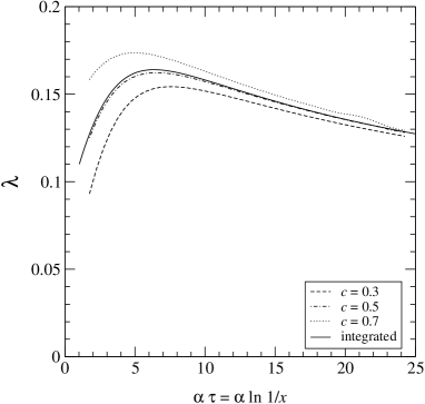
Figure 15: Scheme and $\tau$ dependence of $\lambda$ for one initial condition

Where the form of $N_{\tau,\bm{xy}}$ shows approximate scaling it makes sense to talk about $Q_{s}$ in complete analogy to the fixed coupling case. Again defining the rate of change $\lambda$ according to

$$\lambda(\tau):=\partial_{\tau}\ln Q_{s}(\tau)\ ,$$ (44)

leads to an almost unique and scheme independent quantity. The main new feature is that now, in contrast to the fixed coupling case, $\lambda$ is $\tau$-dependent. Both scheme independence in the near scaling region and $\tau$-dependence of $\lambda$ are shown for one initial condition in Fig. 15. The curves correspond to different values of $c$ in Eq. (39) and a direct definition of $\lambda$ via a moment of the evolution equation to be given below. We see first a strong rise which occurs in the pre scaling region that turns into a slow decrease in the “near” scaling region where the curves converge to a single line. The accuracy to which the the curves agree in the near scaling region at large $\tau$ can be used as a measure of the quality of the scaling.

Since in the scaling region, $Q_{s}(\tau)$ is the only scale left in the problem, it is natural to plot $\lambda(\tau)$ against $R_{s}\sim 1/Q_{s}$. This allows to compare the asymptotic behavior of simulations with different initial conditions as shown in Fig. 16. In this plot we find that all $\lambda$ values obtained from Gaussian initial conditions are limited from above by an asymptotic curve that falls with growing $\tau$ (from left to right in the plot). It is on this asymptotic curve that the scaling shown in Fig. 15 holds.

Figure 16: $\lambda=\partial_{\tau}\ln Q_{s}(\tau)$ for different initial conditions. All curves starting from Gaussian initial conditions stay below an asymptotic line along which we find (approximately) scaling dipole functions $N$.

With the global features established let us turn back to a quantitative analysis of active phase space and a study of the $\tau$ dependence in the near scaling region.

To this end we first show a detailed analysis of the continuum extrapolation of one trajectory at several values in $\tau$ in Fig. 17. On physics grounds we expect the UV cutoff needed in a given case to be determined by $Q_{s}$ at that the $\tau$ considered. In Fig. 17, left, we see that with growing $\tau$ the extrapolations of $\lambda$ towards the continuum limit at the left reach the asymptotic plateau later and later. That this indeed follows $Q_{s}$ is shown in the middle. What remains open in these plots is the precise form of the $\tau$-dependence of $\lambda$. The numerical result here is surprising: our simulations show a clear scaling of $\lambda/\sqrt{\alpha_{s}(Q_{s}(\tau))}$ in the asymptotic region over the range explored in this simulation. This is shown in Fig. 17, right, which summarizes our results on $\tau$ and scale dependence for $\lambda$ in the range of $Q_{s}$ values appearing in this simulation.

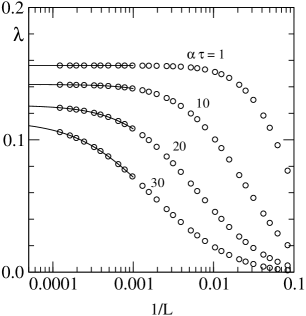
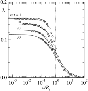
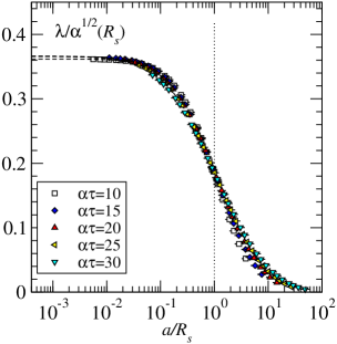
Figure 17: UV dependence of the BK-equation on the asymptotic line after the parent dipole scale is taken to determine the coupling. Left: $\lambda$ against $a$ in units of lattice size. Middle: $\lambda$ against $a$ in units of $R_{s}$, the natural units. Right: the same rescaled by $\sqrt{\alpha_{s}(Q_{s}^{2})}$. Active phase space is limited in the UV (and IR) by $5$ to $10\times Q_{s}$. The $\tau$-dependence of $\lambda$ is, to a good approximation, given by $\lambda(\tau)=\lambda_{0}\sqrt{\alpha_{s}(Q_{s}(\tau)^{2})}$.

Active phase space is clearly centered around $Q_{s}(\tau)$ both in the UV and the IR. The reasons for the boundedness are very different on the two sides: while the IR safety is induced by the nonlinear effects already present at fixed coupling, the limited range into the UV is solely caused by the running of the coupling.

While it is natural to express the $\tau$ dependence of $\lambda$ via $Q_{s}(\tau)$, it is rather surprising that for the small values of the coupling constant in the range covered in Fig. 17 that an expansion of $\lambda$ of the form

$$\lambda(\tau)=c\alpha_{s}(Q_{s}(\tau)^{2})+\text{small corrections}$$ (45)

appears to be totally inadequate and instead a fit of the form

$$\lambda(\tau)=\lambda_{0}\sqrt{\alpha_{s}(Q_{s}(\tau)^{2})}$$ (46)

appears to be surprisingly successful. If the latter provides a good fit, then the corrections in Eq. (45) must be important in the range considered. As it turns out, the fact that $\lambda(\tau)$ can not be expanded in a simple power series in $\alpha_{s}(Q_{s}(\tau)^{2})$ is linked with the large reduction in phase space compared to the fixed coupling case. To see this, let us use an idea by McLerran, Iancu, and Itakura [31] that was introduced in the fixed coupling case to show that there $\lambda$ is necessarily constant in the scaling region.

They assume (in the context of the fixed coupling BK equation) that $N_{\tau\ \bm{xy}}$ depends only on the combination $(\bm{x}-\bm{y})^{2}Q_{s}(\tau)^{2}=:\bm{r}^{2}Q_{s}(\tau)^{2}$. Then $\tau$-derivatives can be traded for $\bm{r}^{2}$ derivatives and the l.h.s. of the BK equation is easily rewritten as

$$\partial_{\tau}N({\bm{r}^{2}Q_{s}(\tau)^{2}})=\bm{r}^{2}\partial_{\bm{r}^{2}}N({\bm{r}^{2}Q_{s}(\tau)^{2}})\partial_{\tau}\ln Q_{s}(\tau)^{2}=\bm{r}^{2}\partial_{\bm{r}^{2}}N({\bm{r}^{2}Q_{s}(\tau)^{2}})2\lambda_{\tau}\ .$$ (47)

Taking into account the spatial boundary conditions imposed by “color transparency”, the fact that $N(\bm{r}^{2}=0)=0$ and $N(\bm{r}^{2}=\infty)=1$, leads us to take the zeroth moment of the BK equation –to integrate with $\frac{d^{2}r}{\bm{r}^{2}}$– in order to isolate $\lambda$ on the l.h.s.. The r.h.s then provides an integral expression for it in form of its zeroth moment:

$$2\pi\lambda(\tau)=\frac{\alpha_{s}N_{c}}{2\pi^{2}}\int\frac{d^{2}rd^{2}z}{\bm{u}^{2}\bm{v^{2}}}\big{(}N(\bm{u}^{2}Q_{s}^{2})+N(\bm{v}^{2}Q_{s}^{2})-N(\bm{v}^{2}Q_{s}^{2})-N(\bm{u}^{2}Q_{s}^{2})N(\bm{v}^{2}Q_{s}^{2})\big{)}$$ (48)

where we have set $\bm{u}=\bm{x}-\bm{z}$ $\bm{v}=\bm{z}-\bm{y}$ for compactness. Due to scale invariance of the integral, the r.h.s. is indeed independent of $\tau$: the scale common to all $N$ can be chosen at will without changing the integral. Indeed, in the scaling region Eq. (48) is completely equivalent to Eq. (44). Outside that region it can be used as an alternative definition of a quantity that gives a qualitative description of the rate of evolution with the same justification as any other definition of $\lambda$ or $Q_{s}$. Its main advantage is that now it is directly related to the integral expression driving the evolution step and we can directly analyze active phase space in this expression where needed.

On the asymptotic line with near scaling the argument is only approximate, but to good accuracy we obtain

$$2\pi\lambda(\tau)=\frac{N_{c}}{2\pi^{2}}\int\frac{d^{2}rd^{2}z}{\bm{u}^{2}\bm{v^{2}}}\alpha_{s}(1/\bm{r}^{2})\big{(}N(\bm{u}^{2}Q_{s}^{2})+N(\bm{v}^{2}Q_{s}^{2})-N(\bm{v}^{2}Q_{s}^{2})-N(\bm{u}^{2}Q_{s}^{2})N(\bm{v}^{2}Q_{s}^{2})\big{)}+\ldots$$ (49)

and we can take the r.h.s. as a definition of $\lambda(\tau)$, ignoring the small corrections. Fig. 15 shows that we indeed agree with the conventionally measured quantity.

Due to the near scaling of $N$ also in the running coupling case together with all other ingredients of the integral, it is really only the presence of the running $\alpha_{s}$ underneath the integral that distinguishes the integrals in Eq. (48) and Eq. (49). To obtain the strong relative reduction in active phase space observed in Fig. 17 we need $\alpha_{s}$ to vary considerably over the range of scales contributing to the integral in the fixed coupling case. Wherever this happens, $\lambda(\tau)$ will be a nontrivial function of $\alpha_{s}(Q_{s}(\tau)^{2})$. Conversely, at asymptotically large $Q_{s}$, where the $\alpha_{s}(1/\bm{r}^{2})$ probed in Eq. (49) turn essentially constant over a range comparable to the phase space needed in the fixed coupling case, we should return to a situation as in Eq. (45). The price to pay is the reopening of phase space to the size encountered already at fixed coupling.

To illustrate this we list active phase space in terms of $a/R$ needed to find $\lambda$ within a given percentage of its continuum value at different $\alpha_{s}(Q_{s}(\tau)^{2})$ in comparison with the fixed coupling result.

deviation from	$\alpha=.2$	$\alpha=.15$	$\alpha=.12$	$\alpha=.1$	fixed coupling
continuum value	$\lambda/\alpha=.845$	$\lambda/\alpha=.96$	$\lambda/\alpha=1.052$	$\lambda/\alpha=1.14$
10%	$a/R=0.17$	$a/R=0.15$	$a/R=0.12$	$a/R=0.1$	$a/R=0.0011$
5 %	$a/R=0.1$	$a/R=0.08$	$a/R=0.066$	$a/R=0.05$	$a/R=0.00013$
1 %	$a/R=0.027$	$a/R=0.015$	$a/R=0.007$	$a/R=0.0012$	$a/R=8.2\cdot 10^{-7}$

Table 1: Phase space needed to extract continuum values for $\lambda$ is reduced for larger values of the coupling. The fixed coupling situation reemerges asymptotically.

In the far asymptotic region we are back to the unsatisfactory situation that we most likely miss important corrections with the additional drawback that we now have no real idea of what those might be. Fortunately, this would appear to occur only at such extremely large values of $Q_{s}$ for this to be purely academic.

With this caveat, we are able to understand the behavior of $\lambda$ on most of the asymptotic line. Fig. 18 shows the behavior of $\lambda$ as a function of $\alpha_{s}(Q_{s}(\tau)^{2})$ and $Q_{s}$ demonstrating in the center the large range over which a fit according to Eq. (46) is successful. To the left of this, we see a deviation that would appear to be consistent with a turnover towards a linear behavior in $\alpha_{s}$. Indeed a purely phenomenological two parameter ansatz of the form

$$\lambda(\tau)=\frac{2.26\alpha_{s}(Q_{s}(\tau)^{2})}{1+a\alpha_{s}(Q_{s}(\tau)^{2})^{b}}$$ (50)

provides a fit consistent with all the available information. Here $2.26$ is the value obtained from the fixed coupling BK-simulation which must emerge due our argument above and $a$ and $b$ have been fitted to be $6$ and $0.8$ respectively.

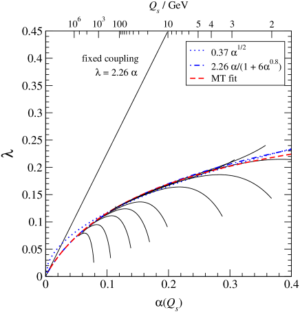
Figure 18: $\lambda(\tau)$ as a function of $\alpha_{s}(Q_{s}(\tau)^{2})$. The central region of the asymptotic line where the running of the coupling reduces phase space is best fitted by a $\lambda(\tau)=\lambda_{0}\sqrt{\alpha_{s}(Q_{s}(\tau)^{2})}$ or equivalently by the use of Eq. (56). At large $Q_{s}$ the curve turns towards a form that allows a perturbative expansion of the form $\lambda(\tau)=c\alpha_{s}(Q_{s}(\tau)^{2})+\text{small corrections}$ at the price of a reopening of phase space.

To establish the link to the asymptotic behavior given in [41, 42], we first observe that the small coupling limit of Eq. (50) with its leading

$$\lambda(\tau)=2.26\alpha_{s}(Q_{s}(\tau)^{2})+\text{small corrections}$$ (51)

is in full agreement with the asymptotic behavior derived in [41, 42]. This we render here as

$$\lambda=\frac{.90}{\sqrt{\tau+Y_{0}}}-\frac{0.47}{(\tau+Y_{0})^{5/6}}+\text{higher inverse powers},$$ (52)

where $Y_{0}$ stands for constants determined by initial conditions. To show agreement with the first term in Eq. (52) analytically, let us consider a generic power like dependence of $\lambda$ on $\alpha_{s}(Q_{s}(\tau)^{2})$ to incorporate both Eq. (51) valid at asymptotically small $\alpha_{s}$ and Eq. (46) which gives a simple representation for the bulk of scales. We make the ansatz

$$\lambda_{\tau}:=\partial_{\tau}\ln(Q_{s}(\tau)/\Lambda_{\text{QCD}})=\lambda_{0}\ \big{[}\alpha_{s}(Q_{s}(\tau)^{2})\big{]}^{n}\hskip 28.45274pt\alpha_{s}(Q_{s}(\tau)^{2}):=\frac{4\pi}{\beta_{0}\ln(Q_{s}(\tau)^{2}/\Lambda_{\text{QCD}})}$$ (53)

with $\beta_{0}=(11N_{c}-2N_{f})/3$, and find

$$\frac{Q_{s}(\tau)^{2}}{\Lambda_{\text{QCD}}^{2}}=\exp\Big{\{}\Big{[}(n+1)2\lambda_{0}\big{(}\frac{4\pi}{\beta_{0}}\big{)}^{n}(\tau-\tau_{0})+\big{[}\ln(\frac{Q_{s}(\tau_{0})^{2}}{\Lambda_{\text{QCD}}^{2}})\big{]}^{n+1}\Big{]}^{\frac{1}{n+1}}\Big{\}}\ .$$ (54)

Recovering $\lambda$ from this we find

$$\lambda(\tau)=\frac{\lambda_{0}\sqrt{\frac{4\pi}{\beta_{0}}}}{\Big{[}(n+1)2\lambda_{0}\sqrt{\frac{4\pi}{\beta_{0}}}(\tau-\tau_{0})+\big{[}\ln(\frac{Q_{s}(\tau_{0})^{2}}{\Lambda_{\text{QCD}}^{2}})\big{]}^{n+1}\Big{]}^{\frac{1}{n+1}-1}}\xrightarrow{n\to 1,\lambda_{0}\to 2.26}\frac{.88}{\sqrt{\tau+Y_{0}}}$$ (55)

so that the leading term of Eq. (52) corresponds to $n=1$ as expected.

To extend the comparison beyond that we simply integrate $\lambda$ in Eq. (52) back to get an expression for $Q_{s}$ and fit the integration constant $c$ to match our simulations. [Alternatively we could have directly used the expressions for $Q_{s}$ in [41, 42] and adjusted the unknown parameter.] We find that

$$\frac{Q_{s}(\tau)}{\Lambda_{\text{QCD}}}=c\cdot\exp[2\cdot 0.9(\tau+Y_{0})^{\frac{1}{2}}-6\cdot 0.47(\tau+Y_{0})^{\frac{1}{6}}]$$ (56)

with $c=1.5$ leads to excellent agreement over the whole range. This is shown in Fig. 18.

To summarize the results of this section we state that Fig. 17 also shows impressively that the contributions to $\lambda$ arise from within little more than an order of magnitude of the saturation scale [the region in cutoffs over which there is an appreciable change in the value extracted]. This indicates that the dominant phase space corrections are indeed taken into account and the basic physics ideas that had initially motivated the density resummations are realized. While the IR side of the resummation was working already at fixed coupling, the UV side of phase space is only tamed if the coupling runs. Only with both the nonlinearities and a running coupling are we justified to claim that the evolution is dominated by distances of the order of $R_{s}$ and thus the coupling involved in typical radiation events during evolution is of order $\alpha_{s}(Q_{S}(\tau)^{2})$. Fig. 18 shows that on the asymptotic line $\lambda(\tau)=\lambda_{0}\sqrt{\alpha_{s}(Q_{s}(\tau)^{2})}$ over most of the region where running coupling limits phase space.

5 Evolution and $A$-dependence

It has been argued in the context of the McLerran-Venugopalan model that going to larger nuclear targets (larger nuclear number $A$) ought to have an enhancing effect on the importance of the nonlinearities encountered. If we are at small enough $x$ (high enough energies) for the projectile to punch straight through the target going to a larger target means interaction with more scattering centers as indicated in Fig. 2. Taking these to be color charges located in individual nucleons inside the target nucleus the interaction will occur with more and more uncorrelated color charges the larger the target. Viewed from up front this amounts to a smaller correlation length in the transverse direction. In terms of $Q_{s}$ this would lead to

$$Q_{s}^{A}(\tau)^{2}=A^{\frac{1}{3}}Q_{s}^{p}(\tau)^{2}$$ (57)

without a clear delineation on the $\tau$ values for which this would be appropriate. This simple argument has been uniformly used in [43] to relate cross section- (or $F_{2}$-) measurements on protons at HERA with measurements on nuclei at NMC and E665. Despite the fact that the nuclear data used are at rather small $Q^{2}$ and large $x$ the agreement found was surprisingly good.

In the context of small $x$ evolution such a statement becomes less trivial: the whole idea of deriving a small $x$ evolution equation is based on premise that the logarithmic corrections determining the evolution step are entirely target independent. The only place where target dependence is allowed to enter is the initial condition.

In simple cases, these two notions are not conflicting with each other: indeed a rescaling like in Eq. (57) is fully compatible with fixed coupling evolution on the asymptotic line, where (in the continuum limit)

$$Q_{s}(\tau)=e^{\lambda\tau}Q_{s}(\tau_{0})$$ (58)

with a universal value for $\lambda$, so that a simple rescaling of the properties of the initial condition according to

$$Q_{s}^{A}(\tau_{0})^{2}=A^{\frac{1}{3}}Q_{s}^{p}(\tau_{0})^{2}\$$ (59)

automatically yields Eq. (57) at all $\tau$ declaring it fully compatible with evolution.

At running coupling, however this ceases to be the case. The straightforward physical argument is that evolution is characterized by $\alpha_{s}(Q_{s}^{2})$ which initially for protons is larger than for nuclei because of the difference in saturation scales at the initial condition. In this situation evolution will be faster for smaller targets and eventually catch up with that of the larger ones.

Technically we find that with running coupling (again restricting ourselves to the asymptotic line), we find a $\tau$ dependent $\lambda$ that we may parametrize through some function $f$ of $\alpha_{s}(Q_{s}(\tau)^{2})$ as as in the previous section:

$$\lambda(\tau)=\partial_{\tau}Q_{s}(\tau)=f(\alpha_{s}(Q_{s}(\tau)^{2}))$$ (60)

In this generic case

$$Q_{s}(\tau)=e^{\int^{\tau}_{\tau_{0}}d\tau^{\prime}f(\alpha_{s}(Q_{s}(\tau)^{2})}Q_{(}\tau_{0})$$ (61)

and a rescaling of $Q_{s}^{p}(\tau_{0})^{2}$ will not simply factor out as in Eq. (58). Therefore and a simple rescaling like Eq. (57) will conflict with evolution. All phenomenological fit functions encountered in the previous section share this property which is at the heart of the reasoning used by Mueller in [44] to argue that evolution will eventually erase $A$-dependence in $Q_{s}$.

To illustrate the point, let trace the the memory loss with a simple parametrization like Eq. (53), equivalent to a $\tau$ dependence of $Q_{s}$ according to Eq. (54).

Scaling in the $A$-dependence at $\tau_{0}$ according to $Q_{s}^{A}(\tau_{0})^{2}=A^{\frac{1}{3}}Q_{s}^{p}(\tau_{0})^{p}\$ within Eq. (54)then predicts both $\tau$ and $A$ dependence of the saturation scale.

We find that evolution will indeed strive to wash out $A$-dependence in qualitative agreement with [44]. Indeed, the ratio of saturation scales in the bulk of the region shown in Fig. 18 then behaves like

$$\frac{Q^{A}_{s}(\tau)^{2}}{Q^{p}_{s}(\tau)^{2}}=\frac{\exp{\Big{[}(n+1)2\lambda_{0}\big{(}\frac{4\pi}{\beta_{0}}\big{)}^{n}(\tau-\tau_{0})+\big{[}\ln(\frac{A^{\frac{1}{3}}Q_{s}(\tau_{0})^{2}}{\Lambda_{\text{QCD}}^{2}})\big{]}^{n+1}\Big{]}^{\frac{1}{n+1}}}}{\exp{\Big{[}(n+1)2\lambda_{0}\big{(}\frac{4\pi}{\beta_{0}}\big{)}^{n}(\tau-\tau_{0})+\big{[}\ln(\frac{Q_{s}(\tau_{0})^{2}}{\Lambda_{\text{QCD}}^{2}})\big{]}^{n+1}\Big{]}^{\frac{1}{n+1}}}}\xrightarrow{\tau\to\infty}1\ .$$ (62)

While the parametrization with $n=1/2$ is not applicable at arbitrary large $\tau$, this formula nevertheless gives a reasonable estimate of the rate of convergence within its window of validity. This is plotted in Fig. 19. Clearly larger nuclei suffer stronger “erasing.” It should be kept in mind that realistically one should not expect real world experiments to cover more than a few orders of magnitude in $x$ and hence too large an interval in $\tau-\tau_{0}$.

Figure 19: $A$-dependence for proton saturation scales from 1 to 100 GeV.

The fact that Eq. (46) and the ensuing $\tau$ dependence is only valid on the asymptotic line of Fig. 16 prevents us from making a direct statement about current and future experiments. Such stronger statements require a more thorough study of initial conditions in direct comparison with existing experiments. If dependence on initial conditions can be clarified $A$ dependence can be studied numerically also in the pre-asymptotic region.

6 Conclusions

In this paper we have, for the first time, shown results from a direct numerical implementation of the JIMWLK equations. The simulations have been performed using a Langevin formulation equivalent to the original equations. These then have been implemented numerically using a lattice discretization of transverse space.

Our simulations have been mainly concerned with extracting universal features and asymptotic behavior induced by the equation itself without direct comparisons with data and systematic studies of initial conditions.

We have clearly established infrared stability of the solutions: once provided with an initial condition that furnishes a (density induced) saturation scale, or correlation length $R_{s}\sim 1/Q_{s}$, the solutions are completely insensitive to IR cutoffs sufficiently below that scale. Such behavior had already been found in the large $N_{c}$ limit in the context of the BK equation and here merely serves as a consistency check.

Simulations of the BK equation have up to now been only carried out in momentum space, our simulations are the first in coordinate space and thus we are the first to show the approach towards the fixed point at infinite energy with vanishing correlation length directly.

Beyond confirming analytical results already found in [22], we also see the emergence of scaling solutions, extending earlier results from simulations of the BK equation to finite $N_{c}$. Within the class of initial conditions studied these emerge universally already at finite energy.

The initial conditions studied were all transversally homogeneous and did not contain large intrinsic $N_{c}$ violations. We found that JIMWLK evolution did not enhance these to above the percent level. In such a situation the BK equation should provide a good approximation. One should be cautious to generalize this too far: any type of lumpiness in the initial condition, hot spots of any kind, would presumably spoil this feature and the factorization limit would not be adequate.

Simulations of the BK equation had already clearly shown that evolution populates a large range in phase space of tens of orders of magnitude, a fact easily attributable to the random walk property of the BFKL equation which due to density effect is tamed in the IR, but not in the UV. While previous studies have taken this as a given, we were forced by the necessity to work on a coordinate lattice to carefully study the UV properties to obtain a valid continuum extrapolation.

Already within the JIMWLK simulation we again found evidence for enormous active phase space that induced relatively large errors in the continuum extrapolations. Since our initial condition did lead to simulations which respect factorization we were in a position to refine this study by implementing the BK-equation in coordinate space with the same type of lattice regulator used in the JIMWLK simulations. We found excellent agreement between the JIMWLK and BK simulations on finite lattices and were able to confirm that the (constant) evolution rate of the saturation scale on the asymptotic line $\lambda=\partial_{\tau}Q_{s}(\tau)$ gets contributions from the far UV, up to 6 orders of magnitude away. In such a situation one typically expects large logarithmic corrections that need to be resummed. Indeed, from the experience with the BFKL equation at two loop, there was an obvious candidate for the main effect, the running of the coupling.

This leads us to the second part of the paper. Here we studied the effect of a naive implementation of running coupling on the same type of questions as studied above. This has been done in the context of the BK-equations for reasons both of efficiency and principle. The latter will be briefly discussed below.

The main effect of running coupling was to drastically improve the convergence towards the continuum limit over a gigantic range of $Q_{s}$ values between $1$ and well above $100$GeV. [Note that the Golec-Biernat+Wüsthoff fits to HERA data have $Q_{s}$ rise from $1$ to $2$GeV from $x=10^{-2}$ to $10^{-4}$.]

Despite the explicit breaking of scale invariance we find that the dipole function still converges towards a scaling form with all the $\tau$ dependence taken by the saturation scale $Q_{s}(\tau)$.

The evolution rate is effected more strongly: $\lambda(\tau)=\partial_{\tau}\ln Q_{s}(\tau)$ now is necessarily $\tau$ dependent. Within the window of strongly reduced phase space between $1$ and $100$GeV it is well described by a simple fit of the form $\lambda(\tau)=.37\sqrt{\alpha_{s}(Q_{s}(\tau)^{2})}$. This is strongly different from the naive expectation that one should find $\lambda(\tau)=c\alpha_{s}(Q_{s}(\tau)^{2})+\text{small corrections}$. We have numerical and analytical indications that such a behavior would reemerge at extremely large $\tau$ at the price of a reopening of phase space. The explanation for this is simple: as shown in Sec. 4, the running coupling appears in an integral expression for $\lambda$ that reduces to the corresponding fixed coupling expression where the running is weak over phase space active in the integral. Thus a strong reduction in phase space necessarily means that $\alpha_{s}$ can not be factored out of the integral. At extremely large $Q_{s}$, however, the running will slow down sufficiently to allow the fixed coupling features to reemerge. The agreement with [41, 42] on the other hand is excellent.

The running coupling induced $\tau$ dependence of $\lambda$ is responsible for another feature of small $x$ evolution already discussed by Mueller [44], the washing out of the $A$ dependence of $Q_{s}$ inherent to the McLerran-Venugopalan model. Scaling $Q_{s}$ at the initial condition at small $\tau_{0}$ according to the McLerran-Venugopalan rule $Q_{s}^{A}(\tau_{0})^{2}=A^{\frac{1}{3}}Q_{s}^{p}(\tau_{0})^{2}$ before evolution adds gluons in an obviously $A$ independent manner leads to a fully determined $\tau$ and $A$ behavior of $Q_{s}$ in which, because of the smaller $\alpha_{s}$ at larger scales evolution of smaller targets can catch up with that of larger ones. Our simulations give quantitative results on the asymptotic line. Quantitative studies with specific initial conditions are possible.

The studies presented in this paper have shown the feasibility of JIMWLK simulations but at the same time have highlighted the necessity of implementing running coupling corrections to obtain reliable results. In particular the latter has been done with a naive scale setting for the running coupling at the parent dipole size. Here clearly improvements are necessary. A more refined treatment would most certainly lead to modifications of our quantitative results such as the fits obtained for the $\tau$-dependence of $\lambda$, although we expect our qualitative conclusions to remain valid. An example that clearly demonstrates the insufficiently of the scale setting used is the fact that such a treatment would not be possible is that such a scale setting is impossible in the full JIMWLK context. There the closest thing to a parent dipole running would be to set the scale at $1/(\bm{x}-\bm{y})^{2}$ in Eq. (9). This, however, is incompatible with BK parent dipole running as is would simply set the scale to infinity in the $\sigma$ terms of Eq. (23) – a step incompatible with the derivation of the BK-equation. Preliminary studies together with Einan Gardi and Andreas Freund have shown that consistency in this respect can be achieved if one implements running coupling with dispersive methods (as widely used for other reasons in the renormalon context), but further work is necessary to gain thorough understanding of all the issues involved.

Complementary issues like the proper choice of initial conditions and questions of $b$-dependence need to be studied to be able to put comparison with experiment on a sound basis.

Acknowledgements:

This work as been carried out over a long timespan and we wish to thank many people for discussions and input at different stages: Yuri Kovchegov, Einan Gardi, Andreas Freund, Genja Levin, Alex Kovner, and Larry McLerran. In particular, we wish to thank Al Mueller and Dionysis Triantafyllopoulos for discussions about the running coupling results. During part of this work HW was supported by the DFG Habilitanden program.

Appendix A From Fokker-Planck to Langevin formulations, the principle

Although this topic is covered in many textbooks, we find that the presentation is often somewhat oldfashioned and the intimate connection with path-integrals is not always mentioned. Let us therefore begin by demonstrating the relationship of Fokker-Planck and Langevin formulations with the aid of a simple toy example, a particle diffusion problem, that, for ease of comparison, shares some of the features of our problem. The toy model equation is

$$\partial_{\tau}P_{\tau}(\bm{x})=-H_{\text{FP}}\ P_{\tau}(\bm{x})$$ (63)

with a Fokker-Planck Hamiltonian

$$H_{\text{FP}}=\frac{1}{2}i\partial_{\bm{x}}^{\mu}\,\chi_{\mu\nu}(\bm{x})\,i\partial_{\bm{x}}^{\nu}\ .$$ (64)

The particles coordinate $\bm{x}$ in $D$ dimensional space corresponds to the field variables of the original problem and the probability distribution $P_{\tau}$ to $\hat{Z}_{\tau}$. It serves to define correlation function of some operator $O(\bm{x})$ via $\langle O(\bm{x})\rangle_{\tau}=\int d^{D}xO(\bm{x})P_{\tau}(\bm{x})$

Eq. (63) admits a path-integral solution which is, as usual, built up from infinitesimal steps in $\tau$: this is a solution $P(\tau^{\prime},\bm{x}^{\prime};\tau,\bm{x})$ to Eq. (67), with initial condition

$$P(\tau,\bm{x}^{\prime};\tau,\bm{x})=\delta^{(D)}(\bm{x}^{\prime}-\bm{x})$$ (65)

that is composed of many, infinitesimally small steps at times $\tau_{k}:=\tau+k\epsilon$. In this solution, the product rule

$$P(\tau^{\prime},\bm{x}^{\prime};\tau,\bm{x})=\int d^{D}x_{n-1}\ldots d^{D}x_{1}\ P(\tau^{\prime},\bm{x}^{\prime};\tau_{n-1},\bm{x})P(\tau_{n-1},\bm{x}_{n-1};\tau_{n-2},\bm{x}_{n-2})\ldots P(\tau_{1},\bm{x}_{1};\tau,\bm{x})$$ (66)

expresses the finite $\tau^{\prime}-\tau$ solution $P(\tau^{\prime},\bm{x}^{\prime};\tau,\bm{x})$ in terms of infinitesimal steps $P(\tau_{i},\bm{x}_{i};\tau_{i-1},\bm{x}_{i-1})$. Solution with arbitrary initial conditions $P_{\tau_{0}}(\bm{x})$ are then recovered via $P_{\tau}(\bm{x})=\int d^{D}yP(\tau,\bm{x};\tau_{0},\bm{y})P_{\tau_{0}}(\bm{y})$.

The derivation of the infinitesimal step from $\tau_{i-1}$ to $\tau_{i}=\tau_{i-1}+\epsilon$ is textbook material and we omit the step. It reads (the index $i$ on the coordinate also refers to the time step, not to the vector component)

$$P(\tau_{i},\bm{x}_{i};\tau_{i-1},\bm{x}_{i-1})=N\int\!\!d^{D}p_{i}\ e^{-\epsilon\big{(}\frac{1}{2}\bm{p}_{i}^{\alpha}\bm{p}_{i}^{\beta}\chi^{\alpha\beta}(\bm{x}_{i-1})+i\bm{p}_{i}\cdot\big{(}\frac{\bm{x}_{i}-\bm{x}_{i-1}}{\epsilon}-\sigma(\bm{x}_{i-1})\big{)}\big{)}}+{\cal O}(\epsilon^{2})$$ (67)

where $\sigma_{\mu}(\bm{x}):=\frac{1}{2}i\partial_{\bm{x}}^{\alpha}\chi_{\alpha\mu}(\bm{x})$ and $N$ a coordinate independent normalization factor.

From here, the step to the Langevin formulation is trivial: as this expression is quadratic in the momenta we can trivially rewrite it with the help of an auxiliary variable $\bm{\xi_{i}}$ [$i$ again the step label] as

$$P(\tau_{i},\bm{x}_{i};\tau_{i-1},\bm{x}_{i-1})=N\int\!\!d^{D}\xi_{i}\ \sqrt{\det(\chi(\bm{x}_{i}))}\ e^{-\frac{1}{2}\bm{\xi}_{i}\chi^{-1}(\bm{x}_{i})\bm{\xi}_{i}}\ \delta^{D}\big{(}\bm{x}_{i}-[\bm{x}_{i-1}+\epsilon(\bm{\xi}_{i}+\sigma(\bm{x}_{i-1})]\big{)}\ .$$ (68)

The $\delta^{D}(\ldots)$ arises from the momentum integration and determines $\bm{x}_{i}$ in terms of $\bm{x}_{i-1}$ and the correlated noise $\bm{\xi}_{i}$. The equation for $\bm{x}_{i}$,

$$\bm{x}_{i}=\bm{x}_{i-1}+\epsilon(\bm{\xi}_{i}+\sigma(\bm{x}_{i-1})\ ,$$ (69)

is called the Langevin equation. It contains both a deterministic term [the $\sigma(\bm{x}_{i-1})$ term] and a stochastic term [the $\bm{\xi}$ term]. To fully define the problem without any reference to its path-integral nature one then needs to state the Gaussian nature of the (correlated) noise separately. This is often done in textbooks. We find that the path-integral version is much more elucidating.

If, as in our case, $\chi$ factorizes as

$$\chi_{\mu\nu}(\bm{x})={\cal E}_{\mu a}(\bm{x}){\cal E}_{\nu a}(\bm{x})\ ,$$ (70)

a simple redefinition of the noise variable leads to a version of the Langevin formulation with a Gaussian white noise:

$$P(\tau_{i},\bm{x}_{i};\tau_{i-1},\bm{x}_{i-1})=N\int\!\!d^{n}\xi_{i}\ e^{-\frac{1}{2}\bm{\xi}_{i}^{2}}\ \delta^{D}\big{(}\bm{x}_{i}-[\bm{x}_{i-1}+\epsilon({\cal E}(\bm{x}_{i-1})\bm{\xi}_{i}+\sigma(\bm{x}_{i-1})]\big{)}\ .$$ (71)

The correlation is now absorbed into the Langevin equation which reads

$$\bm{x}_{i}=\bm{x}_{i-1}+\epsilon({\cal E}(\bm{x}_{i-1})\bm{\xi}_{i}+\sigma(\bm{x}_{i-1})\ ,$$ (72)

Wherever this form is available, it will be the most efficient version to use in a numerical simulation as the associated white noise can be generated more efficiently then the correlated noise of the more general case.

What is left is to sketch a numerical procedure to implement the solution given in Eqns. (66), (67) using the expressions Eq. (68) or Eq. (71). As a first step we replace the average with the probability distribution $P_{\tau}(\bm{x})$ by an ensemble average

$$\langle O(\bm{x})\rangle_{\tau}=\int\!d^{D}x\ O(\bm{x})\ P_{\tau}(\bm{x})\approx\sum\limits_{U\in{\sf E}[P_{\tau}]}O(\bm{x})$$ (73)

where the ensemble is taken according to the probability distribution $P_{\tau}(\bm{x})$. This we can easily do for the initial condition at $\tau_{0}$. The Langevin equation then allows us to propagate each ensemble member down in $\tau$ by $\epsilon$, thereby giving us a new ensemble at $\tau_{1}=\tau+\epsilon$. Iteration then gives us a chain of ensembles for a discrete set of $\tau_{i}$ that provide an approximation to a set of $P_{\tau_{i}}(\bm{x})$ in that they allow us to measure any correlator $\langle O(\bm{x})\rangle_{\tau}$ according to Eq. (73).

The above clearly shows the nature of “Langevin system” as a way of writing a path-integral solution to a differential equation that is particularly easy to implement. Many often confusing issues, such as the time step discretization issues often discussed, find their natural resolution in this setting.

References

- [1] A. H. Mueller and J.-w. Qiu, Gluon recombination and shadowing at small values of x, Nucl. Phys. B268 (1986) 427.
- [2] A. H. Mueller, Soft gluons in the infinite momentum wave function and the BFKL pomeron, Nucl. Phys. B415 (1994) 373–385.
- [3] A. H. Mueller and B. Patel, Single and double BFKL pomeron exchange and a dipole picture of high-energy hard processes, Nucl. Phys. B425 (1994) 471–488, [hep-ph/9403256].
- [4] L. D. McLerran and R. Venugopalan, Computing quark and gluon distribution functions for very large nuclei, Phys. Rev. D49 (1994) 2233–2241, [hep-ph/9309289].
- [5] L. D. McLerran and R. Venugopalan, Gluon distribution functions for very large nuclei at small transverse momentum, Phys. Rev. D49 (1994) 3352–3355, [hep-ph/9311205].
- [6] L. D. McLerran and R. Venugopalan, Green’s functions in the color field of a large nucleus, Phys. Rev. D50 (1994) 2225–2233, [hep-ph/9402335].
- [7] A. Ayala, J. Jalilian-Marian, L. D. McLerran, and R. Venugopalan, The gluon propagator in nonabelian Weizsacker-Williams fields, Phys. Rev. D52 (1995) 2935–2943, [hep-ph/9501324].
- [8] A. Kovner, L. D. McLerran, and H. Weigert, Gluon production from nonAbelian Weizsacker-Williams fields in nucleus-nucleus collisions, Phys. Rev. D52 (1995) 6231–6237, [hep-ph/9502289].
- [9] A. Ayala, J. Jalilian-Marian, L. D. McLerran, and R. Venugopalan, Quantum corrections to the Weizsacker-Williams gluon distribution function at small x, Phys. Rev. D53 (1996) 458–475, [hep-ph/9508302].
- [10] Y. V. Kovchegov, Non-abelian Weizsaecker-Williams field and a two- dimensional effective color charge density for a very large nucleus, Phys. Rev. D54 (1996) 5463–5469, [hep-ph/9605446].
- [11] I. Balitsky, Operator expansion for high-energy scattering, Nucl. Phys. B463 (1996) 99–160, [hep-ph/9509348].
- [12] Y. V. Kovchegov, Quantum structure of the non-abelian Weizsaecker-Williams field for a very large nucleus, Phys. Rev. D55 (1997) 5445–5455, [hep-ph/9701229].
- [13] J. Jalilian-Marian, A. Kovner, L. D. McLerran, and H. Weigert, The intrinsic glue distribution at very small x, Phys. Rev. D55 (1997) 5414–5428, [hep-ph/9606337].
- [14] J. Jalilian-Marian, A. Kovner, A. Leonidov, and H. Weigert, The BFKL equation from the Wilson renormalization group, Nucl. Phys. B504 (1997) 415–431, [hep-ph/9701284].
- [15] J. Jalilian-Marian, A. Kovner, A. Leonidov, and H. Weigert, The Wilson renormalization group for low x physics: Towards the high density regime, Phys. Rev. D59 (1999) 014014, [hep-ph/9706377].
- [16] J. Jalilian-Marian, A. Kovner, and H. Weigert, The Wilson renormalization group for low x physics: Gluon evolution at finite parton density, Phys. Rev. D59 (1999) 014015, [hep-ph/9709432].
- [17] I. Balitsky, Operator expansion for diffractive high-energy scattering, hep-ph/9706411.
- [18] J. Jalilian-Marian, A. Kovner, A. Leonidov, and H. Weigert, Unitarization of gluon distribution in the doubly logarithmic regime at high density, Phys. Rev. D59 (1999) 034007, [hep-ph/9807462].
- [19] A. H. Mueller, Parton saturation at small x and in large nuclei, Nucl. Phys. B558 (1999) 285–303, [hep-ph/9904404].
- [20] Y. V. Kovchegov, Unitarization of the BFKL pomeron on a nucleus, Phys. Rev. D61 (2000) 074018, [hep-ph/9905214].
- [21] A. Kovner, J. G. Milhano, and H. Weigert, Relating different approaches to nonlinear QCD evolution at finite gluon density, Phys. Rev. D62 (2000) 114005, [hep-ph/0004014].
- [22] H. Weigert, Unitarity at small Bjorken x, Nucl. Phys. A703 (2002) 823–860, [hep-ph/0004044].
- [23] E. Iancu, A. Leonidov, and L. D. McLerran, Nonlinear gluon evolution in the color glass condensate. I, Nucl. Phys. A692 (2001) 583–645, [hep-ph/0011241].
- [24] E. Ferreiro, E. Iancu, A. Leonidov, and L. McLerran, Nonlinear gluon evolution in the color glass condensate. II, Nucl. Phys. A703 (2002) 489–538, [hep-ph/0109115].
- [25] K. Golec-Biernat and M. Wüsthoff, Saturation effects in deep inelastic scattering at low and its implications on diffraction, Phys. Rev. D59 (1999) 014017, [hep-ph/9807513].
- [26] K. Golec-Biernat and M. Wüsthoff, Saturation in diffractive deep inelastic scattering, Phys. Rev. D60 (1999) 114023, [hep-ph/9903358].
- [27] A. M. Stasto, K. Golec-Biernat, and J. Kwiecinski, Geometric scaling for the total cross-section in the low x region, Phys. Rev. Lett. 86 (2001) 596–599, [hep-ph/0007192].
- [28] J.-P. Blaizot, E. Iancu, and H. Weigert, Non linear gluon evolution in path-integral form, hep-ph/0206279.
- [29] K. Golec-Biernat, L. Motyka, and A. M. Stasto, Diffusion into infra-red and unitarization of the BFKL pomeron, hep-ph/0110325.
- [30] M. Braun, Structure function of the nucleus in the perturbative QCD with (BFKL pomeron fan diagrams), Eur. Phys. J. C16 (2000) 337–347, [hep-ph/0001268].
- [31] E. Iancu, K. Itakura, and L. McLerran, Geometric scaling above the saturation scale, Nucl. Phys. A708 (2002) 327–352, [hep-ph/0203137].
- [32] M. A. Braun, Pomeron fan diagrams with an infrared cutoff and running coupling, hep-ph/0308320.
- [33] E. Gotsman, E. Levin, M. Lublinsky, and U. Maor, Towards a new global QCD analysis: Low x DIS data from non- linear evolution, Eur. Phys. J. C27 (2003) 411–425, [hep-ph/0209074].
- [34] V. S. Fadin, M. I. Kotsky, and R. Fiore, Gluon reggeization in qcd in the next-to-leading order, Phys. Lett. B359 (1995) 181–188.
- [35] V. S. Fadin, M. I. Kotsky, and L. N. Lipatov, Gluon pair production in the quasi-multi-regge kinematics, hep-ph/9704267.
- [36] V. S. Fadin, R. Fiore, A. Flachi, and M. I. Kotsky, Quark-antiquark contribution to the BFKL kernel, Phys. Lett. B422 (1998) 287–293, [hep-ph/9711427].
- [37] V. S. Fadin and L. N. Lipatov, BFKL pomeron in the next-to-leading approximation, Phys. Lett. B429 (1998) 127–134, [hep-ph/9802290].
- [38] D. Colferai, Small-x processes in perturbative quantum chromodynamics, hep-ph/0008309.
- [39] R. S. Thorne, NLO BFKL equation, running coupling and renormalization scales, Phys. Rev. D60 (1999) 054031, [hep-ph/9901331].
- [40] R. S. Thorne, The running coupling BFKL anomalous dimensions and splitting functions, Phys. Rev. D64 (2001) 074005, [hep-ph/0103210].
- [41] A. H. Mueller and D. N. Triantafyllopoulos, The energy dependence of the saturation momentum, Nucl. Phys. B640 (2002) 331–350, [hep-ph/0205167].
- [42] D. N. Triantafyllopoulos, The energy dependence of the saturation momentum from RG improved BFKL evolution, Nucl. Phys. B648 (2003) 293–316, [hep-ph/0209121].
- [43] A. Freund, K. Rummukainen, H. Weigert, and A. Schäfer, Geometric scaling in inclusive reactions and nonlinear perturbative QCD, Phys. Rev. Lett. 90 (2003) 222002, [hep-ph/0210139].
- [44] A. H. Mueller, Nuclear A-dependence near the saturation boundary, hep-ph/0301109.