Neutrino Mass Patterns within the See-saw Model from Multi-localization along Extra Dimensions

Abstract

We study a multi-localization model for charged leptons and neutrinos, including the possibility of a see-saw mechanism. This framework offers the opportunity to allow for realistic solutions in a consistent model without fine-tuning of parameters, even if quarks are also considered. Those solutions predict that the large Majorana mass eigenvalues for right-handed neutrinos are of the same order of magnitude, although this almost common mass can span a large range (bounded from above by $\sim 10^{12}{\rm GeV}$). The model also predicts Majorana masses between $\sim 10^{-2}{\rm eV}$ and $\sim 5\ 10^{-2}{\rm eV}$ for the left-handed neutrinos, both in the normal and inverted mass hierarchy cases. This mass interval corresponds to sensitivities which are reachable by proposed neutrinoless double $\beta$ decay experiments. The preferred range for leptonic mixing angle $\theta_{13}$ is: $10^{-2}\lesssim\sin\theta_{13}\lesssim 10^{-1}$, but smaller values are not totally excluded by the model.

PACS numbers: 11.10.Kk, 12.15.Ff, 14.60.Pq, 14.60.St

1 Introduction

One of the profound mysteries in particle physics is the origin of strong mass hierarchy existing among the different generations of quarks and leptons. The Standard Model (SM) generates the measured quark and lepton masses with the dimensionless Yukawa couplings, which are spread over numerous orders of magnitude, so that it does not provide a real interpretation to the observed hierarchical pattern. Hence, the SM fermion mass hierarchy should be explained by an higher energy theory. The most famous example for such a theory is certainly based on the Froggatt-Nielsen mechanism [1]. This mechanism introduces a ‘flavor symmetry’ forbidding most of the Yukawa interactions. However, effective Yukawa couplings are generated by the spontaneous breaking of the additional symmetry. Hence, those couplings are suppressed by different powers of the breaking scale over some fundamental high energy scale.

The recent renewed interest for the physics of extra dimensions [2, 3] has lead to approaches toward the SM fermion mass hierarchy problem completely different from the conventional ones. Those new approaches are attractive as they do not rely on the existence of any new symmetry in the short-distance theory. For example, in a framework inspired by the Randall-Sundrum model [3], the large SM fermion mass hierarchy can be understood by means of the metric “warp” factors [4, 5, 6]. The fermion mass hierarchy can also be generated naturally by permitting the fermion masses to evolve with a power-law dependence on the mass scale, in theories with extra space-time dimensions [7, 8]. Other interesting ideas for solving the mass hierarchy problem with extra dimension(s) can be found in the literature [9, 10, 11, 12].

N. Arkani-Hamed and M. Schmaltz have suggested a particularly original and natural interpretation of the SM fermion mass hierarchy [13]. In the Arkani-Hamed-Schmaltz (AS) scenario, the SM fermions are localized at different positions along extra spatial dimension(s) in which our four-dimensional domain wall has thus a spread. This localization can be achieved by using either non-perturbative effects in string/M theory or field-theory methods. One possible field-theoretical mechanism is to couple the SM fermions to scalar fields which have vacuum expectation values depending on the extra dimension(s). Indeed, it is known that chiral fermions are confined in solitonic backgrounds [14]. One of the effects of having the SM fermions “stuck” at different points in the wall is the following: the relative displacements of the SM fermion wave function peaks produce suppression factors in the effective four-dimensional Yukawa couplings. These suppression factors being determined by the overlaps of SM fermion wave functions (getting smaller as the distance between wave function peaks increases), they can vary with the fermion flavors and thus generate the wanted mass hierarchy.

Some interesting variations of the AS scenario, in which the four-dimensional fermions appear as zero modes trapped in the core of a topological defect, have been studied in [15]. The possibilities of localizing the Higgs field in extra dimension(s) [16] or having different fermion wave function widths [17], that would modify the suppression factors arising in AS models, have also been explored. Furthermore, the AS idea has been considered in the contexts of supersymmetry [18, 19] and the Grand Unified Theories (GUT) [20, 21]. Let us mention finally that the effects of gauge interactions on AS models could help in understanding the quark mass hierarchy [22].

Concrete realizations of the AS scenario have been constructed [23, 24, 25, 26], as we will discuss now. In the case of the existence of only one extra dimension, it has been demonstrated that the experimental values for quark masses and $V_{CKM}$ matrix elements lead to a unique characteristic configuration of the field localization [23]. Concerning the charged lepton sector, only one simple example of wave function positions reproducing the measured charged lepton masses has been given in the literature [23]. Let us now consider the situation where right-handed neutrinos are added to the SM so that neutrinos acquire ordinary Dirac masses after electroweak symmetry breaking, exactly like the quarks and charged leptons. Then, if these right-handed neutrinos are also localized in the domain wall, it is possible to find several field configurations yielding to appropriate neutrino masses and mixing angles for explaining all the experimental neutrino data [24]. However, in this case of Dirac masses for neutrinos, it turns out that the positions of neutrino fields are closely related [24]. This fine-tuning problem for the fundamental parameters is mainly due to the large leptonic mixing angles required by neutrino oscillation solutions to the neutrino puzzle [27], and thus does not appear in the quark sector.

In the present work, we investigate the alternative possibility that, within the AS scenario, neutrinos acquire masses of Majorana type (instead of Dirac type as previously studied). We concentrate on the ‘see-saw’ model [28] which constitutes probably the most elegant way of generating Majorana neutrino masses. The whole leptonic sector is considered, since the neutrino and charged lepton sectors are related phenomenologically through the data on leptonic mixing angles, and, theoretically via the field positions in the wall of left-handed $SU(2)_{L}$ doublets of leptons. Furthermore, we restrict ourselves to the minimal case where the domain wall is thick in only one of the extra dimensions.
In this study, we address the question of the existence of field localization configurations fitting all the present experimental data on charged leptons and neutrinos. In other words, we are interested in the structure of lepton flavor space. We will show that it is indeed possible to find wave function displacement configurations in agreement with experimental results, and we will present complete realistic AS models.
First, a general description of the less fine-tuned solutions reproducing the charged lepton masses will be given. Then, within this context, we will show that the fine-tuning of neutrino field positions, which has appeared in the case of Dirac masses for neutrinos [24], is softer in the see-saw framework considered here. The reasons will be exposed in details. This result that the fine-tuning reaches an acceptable level in the whole leptonic sector, which was the most serious phenomenological challenge for the AS scenario [24], makes this kind of AS model a realistic candidate for the solution to the mass hierarchy problem.
Moreover, it will be pointed out that the studied model, namely the see-saw mechanism within the AS scenario, gives rise to clear predictions on the value of light neutrino masses and to favored values for the leptonic mixing angle $\theta_{13}$. Those predictions are interesting since they will be testable in the next generation of terrestrial neutrino experiments, as will be discussed.
Finally, we will illustrate that, within this model, the reduction of neutrino masses compared to the electroweak symmetry breaking scale can be due partially to the see-saw mechanism, and partially to the suppression factors issued from field localization effect. Therefore, the field positions can be closer to each other than in the case of neutrino Dirac masses where the mass reduction comes entirely from the localization effect. This is attractive for two reasons. First, it renders the upper bound on the wall width, coming from perturbativity considerations, easier to respect. Secondly, it pleads for the ‘naturality’ of the AS scenario, in the sense that generating large mass hierarchies from field positions (namely combinations of the fundamental parameters) of the same order of magnitude can be considered as a satisfactory and natural property. This property is maybe the main progress brought by the AS scenario with regard to the SM fermion mass hierarchy problem.

At this level, one should mention a preliminary study on the same subject, performed in [29], even if the approach adopted was much less generic than here: the authors of [29] have considered, within the AS scenario, the combination of the see-saw mechanism together with a model containing a triplet Higgs scalar, in view of predicting a degenerate diagonal neutrino mass spectrum. Such a spectrum allows a neutrino contribution to the hot component of the dark matter of the universe. Let us note that the authors of [29] have given the example of a model reproducing the experimental data on leptons, in the context of the see-saw mechanism within the AS framework. However, this example concerns a two extra dimension version of the model, and is associated to the small mixing angle solution of the solar neutrino problem which has been ruled out by the recent experimental results [27].

In another interesting previous related work [30], the AS scenario has been mentioned as a possible natural framework, for justifying the neutrino texture of a particular well motivated see-saw model. This approach of the AS scenario was thus purely effective, in the two following senses. First, the fundamental parameters, namely the field positions, were replaced by effective neutrino mass parameters. Secondly, the charged lepton sector, which is not independent of the neutrino sector within the AS framework (see above), was not fully treated. We will come back on the study of [30] later.

A last comment may be done at this stage. As already said, the scenario we will study can explain both the structure in neutrino flavor space and the (partial) suppression of neutrino mass scales compared to the electroweak scale, in terms of geometrical patterns in an higher-dimensional space. There exist two other types of scenarios based on the existence of extra dimension(s) which offer the opportunity to explain the smallness of neutrino masses. Nevertheless, these scenarios do not provide interpretations of the neutrino flavor structure. In the first type of scenario, the lepton number breaking occurs on distant branes and is conveyed to our ‘3-brane’ by a scalar field, leading then to weak effective neutrino Majorana masses [31, 32, 33]. In the other kind of model, the right-handed neutrinos live in the bulk which gives rise to small neutrino Dirac masses, for the same reason that gravity is weak at low energy in this context [31, 32].

In Section 2, we discuss the see-saw mechanism within the context of the AS framework. Then, in Sections 3 and 4, we construct consistent realizations of the AS scenario reproducing all the present experimental data on the whole leptonic sector, in the cases of 2 and 3 flavors respectively. Finally, in Section 5, we present predictions on neutrino sector provided by the AS scenario based on the see-saw mechanism.

2 The See-saw Mechanism within the AS Framework

2.1 The AS scenario

We briefly recall here the physical context and formalism of the AS scenario. The SM degrees of freedom live on a four-dimensional wall embedded in an higher-dimensional space where gravity, and possibly other gauge singlet fields, are free to propagate. We consider the simple case where the domain wall is slightly thick in only one extra dimension. Inside our wall, the Higgs and gauge bosons are free to propagate whereas the SM fermions of each family are trapped at different points. In an effective field theory approach, this field localization can be due to the coupling of each fermion $\Psi_{i}(x_{\mu},x_{5})\ [i=1,...,3;\mu=1,...,4]$ to a five-dimensional scalar field having a vacuum expectation value $\Phi_{i}(x_{5})$ which varies along the extra dimension (parameterized by $x_{5}$). Under the hypothesis that the scalar field profile behaves as a linear function of the type $\Phi_{i}(x_{5})=2\mu^{2}x_{5}-m_{i}$ around its zero-crossing point $x^{0}_{i}=m_{i}/2\mu^{2}$, the zero mode of the five-dimensional fermion $\Psi_{i}(x_{\mu},x_{5})$ acquires a gaussian wave function of typical width $\mu^{-1}$ and centered at $x^{0}_{i}$ along the $x_{5}$ direction:

$$\Psi^{(0)}_{i}(x_{\mu},x_{5})=Ae^{-\mu^{2}(x_{5}-x^{0}_{i})^{2}}\psi_{i}(x_{\mu}),$$ (1)

$\psi_{i}(x_{\mu})$ being a four-dimensional fermion field and $A=(2\mu^{2}/\pi)^{1/4}$ the normalization factor.

Within such a situation, the effective four-dimensional Yukawa couplings between the five-dimensional SM Higgs boson $H$ and zero mode fermions, obtained by integration on $x_{5}$ over the wall width $L$:

$${\cal S}_{Yukawa} = \int d^{5}x\sqrt{L}\kappa H(x_{\mu},x_{5})\bar{\Psi}^{(0)}_{i}(x_{\mu},x_{5})\Psi^{(0)}_{j}(x_{\mu},x_{5})$$ (2)

$$= \int d^{4}x\lambda_{ij}h(x_{\mu})\bar{\psi}_{i}(x_{\mu})\psi_{j}(x_{\mu}),$$ (3)

are modulated by the following coupling constants,

$$\lambda_{ij}=\int dx_{5}\kappa A^{2}e^{-\mu^{2}(x_{5}-x^{0}_{i})^{2}}e^{-\mu^{2}(x_{5}-x^{0}_{j})^{2}}=\kappa e^{-{\mu^{2}\over 2}(x^{0}_{i}-x^{0}_{j})^{2}}.$$ (4)

In this context, it can be considered as natural to have a dimensionless Yukawa coupling constant $\kappa$ which is universal and approximately equal to unity at the electroweak scale, and to generate entirely the flavor structure of effective Yukawa couplings $\lambda_{ij}$ by field localization effects through the exponential suppression factor of Eq.(4).

2.2 Application to the See-saw Model

Let us apply the AS scenario to the lepton sector. The SM charged lepton mass hierarchy can effectively be interpreted by means of field localization. Indeed, if the zero modes for the five-dimensional fields of charged lepton doublets (singlets) under $SU(2)_{L}$ are localized at the positions $l_{i}$ ($e_{j}$) along the wall width, then the effective four-dimensional Dirac mass terms can be written as,

$${\cal L}^{(l^{\pm})}_{Mass}=m^{l^{\pm}}_{ij}\bar{e}^{c}_{Li}e^{c}_{Rj}+h.c.,$$ (5)

where $e_{Li}$ ($e_{Ri}$) denotes the four-dimensional field of the left(right)-handed charged lepton and the mass matrix reads as (see Eq.(4)),

$$m^{l^{\pm}}_{ij}=\rho e^{-{\mu^{2}\over 2}(l_{i}-e_{j})^{2}},\ \mbox{with}\ \rho=\kappa\langle h\rangle,$$ (6)

$\langle h\rangle$ being the vacuum expectation value of the SM Higgs boson.

We now turn to the neutrino sector, assuming that the neutrino masses result from a see-saw mechanism. Let us recall the basics of the see-saw model. In this model, a right-handed neutrino $N_{R}$, which is a Majorana particle, is added to the SM. Then the Lagrangian must contain all the additional mass terms involving $N_{R}$ consistent with the SM gauge invariance, which are the following,

$${\cal L}_{See-saw}=m^{\nu}_{Dij}\bar{\nu}^{c}_{Li}N^{c}_{Rj}+{1\over 2}M_{ij}\bar{N}_{Ri}N^{c}_{Rj}+h.c.,$$ (7)

where $\nu_{Li}$ denotes the left-handed neutrino of the SM. The first term of Eq.(7) represents a Dirac mass issued from the spontaneous electroweak symmetry breaking, whereas the second term constitutes a Majorana mass originating from a physics underlying the SM. This difference of origins allows the Majorana masses to be much larger than the Dirac masses, a feature that is required by the see-saw mechanism. Under this assumption and after a unitary transformation, the Lagrangian (7) can be rewritten in the mass basis as,

$${\cal L}^{(\nu)}_{Mass}={1\over 2}m^{\nu}_{ij}\bar{\nu}^{c}_{Li}\nu_{Lj}+{1\over 2}M_{ij}\bar{N}_{Ri}N^{c}_{Rj}+h.c.,$$ (8)

where the Majorana mass matrix $m^{\nu}$ is given by the famous see-saw formula [34]:

$$m^{\nu}\simeq-m^{\nu}_{D}M^{-1}m^{\nu\ T}_{D}.$$ (9)

The flavor structure of the Dirac and Majorana mass matrices in Eq.(7), and thus of the neutrino mass matrix given by the see-saw formula (9), can be explained by an AS model. For that purpose, the zero modes of the five-dimensional fields of both left and right-handed neutrinos must be localized at different positions along the wall width. Indeed, in this case, the Dirac mass matrix of Eq.(7) reads as,

$$m^{\nu}_{Dij}=\rho e^{-{\mu^{2}\over 2}(l_{i}-N_{j})^{2}},$$ (10)

exactly like the Dirac mass matrix of charged leptons (see Eq.(6)). The parameter $N_{j}$ in Eq.(10) is the position of the right-handed neutrino. Notice that the left-handed charged lepton and left-handed neutrino are confined at the same point $l_{i}$ (see Eq.(6) and Eq.(10)). It is due to the fact that the whole $SU(2)_{L}$ doublet of leptons is stuck at the point $l_{i}$. Furthermore, in a context of field localization, the Majorana mass matrix of Eq.(7) is given by,

$$M_{ij}=M_{R}e^{-{\mu^{2}\over 2}(N_{i}-N_{j})^{2}}.$$ (11)

In analogy with the Dirac mass matrices of Eq.(6) and Eq.(10), We have assumed a common mass scale factor ($M_{R}$) in the Majorana mass matrix (11). In this way, the flavor structure of mass matrix $M_{ij}$ is completely dictated by field displacement effects. To obtain the see-saw formula within the AS framework, we replace in Eq.(9) the Dirac and Majorana mass matrices by their expression respectively in Eq.(10) and Eq.(11). This leads to the result:

$$m^{\nu}_{ij}\simeq-{\rho^{2}\over M_{R}}e^{-{\mu^{2}\over 2}(l_{i}-N_{a})^{2}}\bigg{[}e^{-{\mu^{2}\over 2}(N_{a^{\prime}}-N_{b^{\prime}})^{2}}\bigg{]}_{ab}^{-1}e^{-{\mu^{2}\over 2}(N_{b}-l_{j})^{2}},$$ (12)

where there is an implicit sum over the $a$ and $b$ indices and the exponent $-1$ must be taken in the sense of the inverse of a matrix. The effective mass matrix of Eq.(12) is the neutrino mass matrix we will study. Its expression is given explicitly in Appendix A, for the case of two lepton flavors ($\{i,j\}=2,3$).

2.3 Energy Scales

The three characteristic energy scales of the AS scenario are the fundamental scale (in a five-dimensional space-time) $M_{\star}^{5D}$ and the energy scales $\mu$ and $L^{-1}$ introduced in Section 2.1.
Let us describe the conditions that these energy scales must fulfilled. First, $\mu$ must be smaller than the fundamental energy scale. Moreover, the four-dimensional effective top quark Yukawa coupling has to remain perturbative up to the fundamental scale. These two conditions imply the following scale relation,

$$\mu<M_{\star}^{5D}\lesssim 1000L^{-1}.$$ (13)

Besides, for the AS mechanism to make sense, it is necessary that the wall thickness is larger than the typical width of gaussian wave functions $\mu^{-1}$. Furthermore, if a field-theoretic description is to work throughout the domain wall, one must have $\Phi_{i}(L/2)\sim\mu^{2}L<M_{\star}^{5D}$. These two new conditions together with Eq.(13) lead to,

$$\mu^{-1}\lesssim L\lesssim 30\mu^{-1}.$$ (14)

Now, we discuss the value of typical Majorana mass scale $M_{R}$ characteristic of the see-saw model (see Section 2.2), within an AS framework. The inequalities (13) and (14), which summarize the conditions on the three energy scales of AS scenario, only constrain ratios of scales and not the scales themselves. Therefore, we can assume that the fundamental scale $M_{\star}^{5D}$ possibly reaches much larger values than the electroweak scale (as it was done in [20] for instance). Our motivation is to allow the free parameter $M_{R}$ to run over a wide range of orders of magnitude, in order to study the different modes of the see-saw mechanism. Since we want to suppose a large fundamental scale, let us take it higher than the GUT scale: $M_{\star}^{5D}>M_{GUT}\simeq 10^{16}{\rm GeV}$. In this way, the scale of physics beyond the SM, $\Lambda$, which enters the non-renormalizable operators of type $(ql)^{\dagger}(u^{c}d^{c})/\Lambda^{2}$, mediating proton decay, can be assumed larger than the GUT scale. This guarantees that the experimental limit on proton lifetime, namely $\tau_{proton}\gtrsim 3\ 10^{33}\ years$, is well verified. Besides, for $M_{\star}^{5D}\gtrsim 10^{16}{\rm GeV}$, it is clear from Eq.(13) that the most severe experimental bound on the wall width [35],

$$L^{-1}\gtrsim 100{\rm TeV},$$ (15)

which comes from considering flavor changing neutral currents (FCNC) mediated by Kaluza-Klein excitations of gauge bosons, is respected.

Let us specify here our motivations for considering a large fundamental mass scale $M_{\star}^{5D}$ (at the end of our analysis, we will discuss the implications of a low $M_{\star}^{5D}$ scale hypothesis).
First, having an high fundamental scale allows to study the case of $M_{R}$ values much larger than the electroweak scale $\rho$ (see Eq.(6)). In this case, the neutrino mass suppression relatively to $\rho$ (see Eq.(12)) comes more from the factor $\rho/M_{R}$ (due to the see-saw mechanism) than from the exponential factors (due to the field localization effects). Such a situation (see end of Section 3.4) is interesting since it gives rise to leptonic field positions significantly closer to each other than in the case of neutrino Dirac masses (see Eq.(10)) where the neutrino mass reduction only originates from localization effects.
Secondly, the proton stability can then be ensured by the existence of large energy scales ($\Lambda\gtrsim 10^{16}{\rm GeV}$). Hence, no suppression of the coupling constants, associated to non-renormalizable operators violating both lepton and baryon numbers, is required from confinement of quarks and leptons at far positions in the extra dimension (as proposed by the authors of [13]).
Similarly, the experimental constraints on FCNC processes are then respected thanks to the presence of large mass scales (see Eq.(15)). Therefore, no suppression factors are required from constraining the distances between field positions of each quark or lepton generation (as suggested in [24] for suppressing the rates of FCNC decays: $l^{\pm}_{i}\to l^{\pm}_{j}\gamma$ and $l^{\pm}_{i}\to l^{\pm}_{j}l^{\pm}_{j}l^{\mp}_{j}$ [$i\neq j$]).
In summary, choosing an high fundamental scale $M_{\star}^{5D}$ permits typically to have closer field positions along the wall. This proximity of the fields has two main interests. First, it is in favor of the naturality of the AS scenario, as explained in Section 1. Secondly, it makes the condition on wall thickness $L\lesssim 30\mu^{-1}$ (see Eq.(14)), due to considerations on perturbativity, easier to fulfill, when one is constructing realistic AS models as we are going to do in the following.

3 Realistic AS Models with 2 Flavors

In this part, we search for the configurations of leptonic field localizations in the domain wall which reproduce all the present experimental data, within the context of AS scenario. More precisely, we try to find the values of field positions $e_{i},l_{j},N_{k}$ and Majorana mass scale $M_{R}$ (see Section 2.2) being consistent with the known constraints on both neutrinos and charged leptons. As already said, we consider the situation where neutrinos acquire masses through the see-saw mechanism.

For a better understanding of observable quantity dependence on fundamental parameters $e_{i},l_{j},N_{k}$ and $M_{R}$, we first treat the case of 2 lepton flavors in this part and then the realistic case of 3 flavors in Section 4. Hence, in this part, the flavor indices of $e_{i},l_{j}$ and $N_{k}$ run over the last two families: $\{i,j,k\}=2,3$ (the flavor indices hold in the flavor basis).

Besides, in order to impose the experimental constraints progressively, and thus to restrict our analysis to the relevant regions of theoretical parameter space $\{e_{i},l_{j},N_{k},M_{R}\}$, we proceed through a three step approach: we first treat the charged lepton masses, then the leptonic mixing angles (which are constrained by neutrino oscillation observations) and finally the neutrino masses.

3.1 Charged Lepton Masses

3.1.1 Notations and conventions

The physical charged lepton masses are derived from a bi-unitary transformation of the mass matrix, namely $m^{l^{\pm}}_{ij}$ (see Eq.(6)):

$$m^{l^{\pm}}=U_{lL}^{\dagger}\left(\begin{array}[]{cc}m_{\mu^{\pm}}&0\\ 0&m_{\tau^{\pm}}\end{array}\right)U_{lR},$$ (16)

where $L/R$ corresponds to charged lepton chirality (see Eq.(5)). A useful method for computing the charged lepton masses is to diagonalize the hermitian square of mass matrix:

$$m^{l^{\pm}}m^{l^{\pm}\ \dagger}=U_{lL}^{\dagger}\left(\begin{array}[]{cc}m^{2}_{\mu^{\pm}}&0\\ 0&m^{2}_{\tau^{\pm}}\end{array}\right)U_{lL}.$$ (17)

The unitary matrix $U_{lL}$ can be parameterized by a mixing angle $\theta_{l}$ like,

$$U_{lL}=\left(\begin{array}[]{cc}\cos\theta_{l}&\sin\theta_{l}\\ -\sin\theta_{l}&\cos\theta_{l}\end{array}\right).$$ (18)

3.1.2 Solutions

Which configurations of the field positions $l_{i}$ and $e_{j}$ give rise to a mass matrix $m^{l^{\pm}}_{ij}$ (see Eq.(6)) in agreement with the measured values of physical charged lepton masses (see Eq.(17)) ? The configurations of this kind corresponding to a minimum fine-tuning of the parameters $l_{i}$ and $e_{j}$ are associated to the following textures of charged lepton mass matrices,

$$m^{l^{\pm}}_{I}\simeq\left(\begin{array}[]{cc}m_{\alpha}&0\\ 0&m_{\beta}\end{array}\right),\ m^{l^{\pm}}_{II}\simeq\left(\begin{array}[]{cc}0&m_{\alpha}\\ m_{\beta}&0\end{array}\right),$$ (19)

$m_{\alpha,\beta}$ being the experimental values of charged lepton masses: $\{m_{\alpha},m_{\beta}\}=m^{exp}_{\mu^{\pm}},m^{exp}_{\tau^{\pm}}$. This result will be shown numerically at the end of this Section, and it can be understood as follows. First, the textures of Eq.(19) reproduce well the measured charged lepton masses, as it is clear in the example of the diagonal case:

$$m^{l^{\pm}}_{I}\simeq\left(\begin{array}[]{cc}m^{exp}_{\mu^{\pm}}&0\\ 0&m^{exp}_{\tau^{\pm}}\end{array}\right)\ \Rightarrow\ m^{l^{\pm}}_{I}m^{l^{\pm}\ \dagger}_{I}\simeq U_{lL}^{\dagger}\left(\begin{array}[]{cc}m^{exp\ 2}_{\mu^{\pm}}&0\\ 0&m^{exp\ 2}_{\tau^{\pm}}\end{array}\right)U_{lL},\ U_{lL}\simeq{\bf 1}_{2\times 2}.$$ (20)

Secondly, the textures in Eq.(19) correspond to a minimal fine-tuning of $l_{i}$ and $e_{j}$ since they impose only one specific condition per parameter. For instance, in the diagonal case, the only mass relation that the parameter $l_{2}$ has to verify is (see Eq.(6) and Eq.(20)),

$$m^{exp}_{\mu^{\pm}}=\rho e^{-{\mu^{2}\over 2}(l_{2}-e_{2})^{2}}.$$ (21)

We also see on this example that the choice in the sign of quantity $l_{i}-e_{j}$ entering Eq.(6) is arbitrary, leading thus to different types of acceptable field position configurations.

All the observable quantities (masses,…) are invariant under some trivial transformations of the localization configurations. For instance, the physical quantities are left invariant by a simultaneous translation of all the field positions along the domain wall. This is due to the fact that the mass matrices involve only some differences of the positions (see Eq.(6)). Therefore, in order to not consider localization configurations which are physically equivalent to each other, we fix the value for one of the positions: $e_{2}=0$. In the example of diagonal charged lepton mass matrix described above, this choice leads to the relation,

$$m^{exp}_{\mu^{\pm}}=\rho e^{-{\mu^{2}\over 2}l_{2}^{2}},$$ (22)

which gives the absolute value of parameter $l_{2}$.
Similarly, there is an invariance under the symmetry $X_{i}\to-X_{i}$, $X_{i}$ representing all the field positions. This one comes from the fact that only some squares of position differences enter the mass matrices (see Eq.(6)). Hence, for the same reason as before, we fix the sign for one of the $l_{i}$ parameters. In the example of diagonal mass matrix, we would fix the sign of $l_{2}$ so that this parameter would be completely determined:

$$l_{2}=\mu^{-1}\sqrt{-2\ln(m^{exp}_{\mu^{\pm}}/\rho)}.$$ (23)

In summary, eliminating physically equivalent localization configurations allows to determine one of the $l_{i}$ parameters, if one considers the charged lepton textures of Eq.(19).

3.1.3 Mass uncertainty

Although the charged lepton masses are known up to an high precision, it is more reasonable to consider an existing significant uncertainty on the measured values of those masses. The three reasons are the following. First, the goal of our analysis is not to find the values of acceptable field positions with an high accuracy. Secondly, a non-negligible error on observable quantities must be introduced if the fine-tuning of fundamental parameters is to be discussed. The third reason has to do with the fact that the running of lepton masses with the energy scale must be taken into account in the analysis. In order to study lepton mass hierarchies which are not affected by renormalization effects (for simplicity), we consider all the mass values at a common energy scale of the order of electroweak scale, namely the top quark mass $m_{top}$. Therefore, the theoretical predictions for lepton mass values are computed with (see Eq.(6)),

$$\rho=\rho(m_{top})=\kappa(m_{top})\langle h\rangle=1.5m_{top}(m_{top}),$$ (24)

where the mass of the top quark evaluated at its own mass scale in the $\overline{MS}$ scheme is $m_{top}(m_{top})=166\pm 5{\rm GeV}$, following the studies of [23, 24]. The choice of $\rho(m_{top})$ value is motivated by the facts that the AS mechanism works for $\rho\geq m_{top}$ and that considerations on naturalness and perturbativity lead to a coupling constant $\kappa(m_{top})$ close to unity (see Section 2.1 and discussion in [23]). This choice does not affect our results and predictions as we will discuss later (Section 5.1). Since the experimental values of lepton masses and their theoretical predictions must be compared at an identical energy scale, the measured lepton masses have also to be taken at the top mass scale. Nevertheless, the effect on the charged lepton masses of running from the pole mass scale up to the top mass scale is only of a few percents [23]. Hence, for the experimental values of charged lepton masses, we take the pole masses [36] and we assume an uncertainty of $5\%$: $\delta m^{exp}_{l^{\pm}}/m^{exp}_{l^{\pm}}=0.05$.

In case of a significant uncertainty on the measured values of charged lepton masses, there is a possible deviation from the textures considered in Eq.(19) which reproduce the correct masses. Let us consider once more the example of diagonal case: the existence of uncertainties on experimental charged lepton masses allows a continuous variation from the realistic texture in Eq.(20):

$$m^{l^{\pm}}_{I}=\left(\begin{array}[]{cc}m^{exp}_{\mu^{\pm}}+\epsilon_{1}&\epsilon_{2}\\ \epsilon_{3}&m^{exp}_{\tau^{\pm}}+\epsilon_{4}\end{array}\right)\ \Rightarrow\ m^{l^{\pm}}_{I}m^{l^{\pm}\ \dagger}_{I}=U_{lL}^{\dagger}\left(\begin{array}[]{cc}m^{exp\ 2}_{\mu^{\pm}}+\delta_{1}&\delta_{2}\\ \delta_{3}&m^{exp\ 2}_{\tau^{\pm}}+\delta_{4}\end{array}\right)U_{lL},$$ (25)

$\epsilon_{i}$ and $\delta_{i}$ representing mass variations. The localization configurations associated to texture (25), which give rise to a minimum fine-tuning of parameters $l_{i}$ and $e_{j}$, correspond to $\delta_{2},\delta_{3}\ll m^{exp\ 2}_{\mu^{\pm}},m^{exp\ 2}_{\tau^{\pm}}$ with $\delta_{1}\in[-\delta m^{exp\ 2}_{\mu^{\pm}},+\delta m^{exp\ 2}_{\mu^{\pm}}]$ and $\delta_{4}\in[-\delta m^{exp\ 2}_{\tau^{\pm}},+\delta m^{exp\ 2}_{\tau^{\pm}}]$, leading to $\theta_{l}\approx 0$ (see Eq.(18)), as it will be shown in Section 3.2. The reason is that the presence of non-negligible contributions to $m^{l^{\pm}}_{I}m^{l^{\pm}\ \dagger}_{I}$ from $\delta_{2,3}=f(\epsilon_{i})=g(l_{i},e_{j})$ ($f$ and $g$ being certain functions) would give rise to new specific relations involving $l_{i}$ and $e_{j}$, and would thus increase their fine-tuning.
In conclusion, even with significant uncertainties on measured charged lepton masses, the less fine-tuned solutions of field positions $l_{i}$ and $e_{j}$ associated to textures in Eq.(19) lead to: $\theta_{l}\approx 0$ for $[m_{\alpha}=m^{exp}_{\mu^{\pm}};m_{\beta}=m^{exp}_{\tau^{\pm}}]$ and $\theta_{l}\approx\pi/2$ for $[m_{\alpha}=m^{exp}_{\tau^{\pm}};m_{\beta}=m^{exp}_{\mu^{\pm}}]$. This result can be understood like this: requiring a given large mixing in the charged lepton sector constitutes an additional specific condition on $l_{i}$ and $e_{j}$, and thus tends to increase their fine-tuning.

3.1.4 Scan

By performing a simultaneous scan on the parameters $l_{2},l_{3}$ and $e_{3}$ ($e_{2}=0$ as explained before) with a step of $10^{-2}$ in the ranges $l_{2},l_{3}\in[-15\mu^{-1},15\mu^{-1}]$ and $e_{3}\in[-20\mu^{-1},20\mu^{-1}]$ (this choice is motivated by Eq.(14)), we find that all the localization configurations reproducing the wanted charged lepton masses correspond to the following textures,

$$m^{l^{\pm}}_{I}\simeq\left(\begin{array}[]{cc}m_{\alpha}&\epsilon_{1}\\ \epsilon_{2}&m_{\beta}\end{array}\right),\ m^{l^{\pm}}_{II}\simeq\left(\begin{array}[]{cc}\epsilon_{1}&m_{\alpha}\\ m_{\beta}&\epsilon_{2}\end{array}\right),$$ (26)

$m_{\alpha,\beta}$ being defined as in Eq.(19), with $\theta_{l}\approx 0$ or $\theta_{l}\approx\pi/2$. This result shows that the typically less fine-tuned solutions, for field positions $l_{i}$ and $e_{j}$, correspond indeed to continuous deviations (because of the significant mass uncertainty) from the textures (19) with $\theta_{l}\approx 0$ or $\pi/2$. For instance, one class of solutions, reproducing the correct charged lepton masses, that we find via the scan described previously reads as,

$$\bigg{\{}e_{2}=0;\ e_{3}\simeq l_{3}+\mu^{-1}\sqrt{-2\ln(m^{exp}_{\tau^{\pm}}/\rho)};\ l_{2}\simeq\mu^{-1}\sqrt{-2\ln(m^{exp}_{\mu^{\pm}}/\rho)};$$ (27)

$$l_{3}\in[-15,-3.61]\mbox{U}[4.41,15]\ (\mbox{in units of}\ \mu^{-1})\bigg{\}}.$$ (28)

This type of solutions corresponds (see Eq.(6)) to the texture $m^{l^{\pm}}_{I}$ of Eq.(26) with $m_{\alpha}=m^{exp}_{\mu^{\pm}}$, $m_{\beta}=m^{exp}_{\tau^{\pm}}$ and $e_{3}-l_{3}>0$ (the sign of $l_{2}$ being fixed in order to eliminate the equivalent solutions obtained by the action of symmetry $X_{i}\to-X_{i}$).

3.1.5 Conclusion

In summary, the less fine-tuned solutions for field positions $l_{i}$ and $e_{j}$, reproducing the measured charged lepton masses, are divided into 8 types of solutions corresponding to: 2 kinds of matrix texture (see Eq.(26)) $\times$ 2 mass permutations ($[m_{\alpha}=m^{exp}_{\mu^{\pm}};m_{\beta}=m^{exp}_{\tau^{\pm}}]$ or $[m_{\alpha}=m^{exp}_{\tau^{\pm}};m_{\beta}=m^{exp}_{\mu^{\pm}}]$) $\times$ 2 opposite signs (for one of the differences $l_{i}-e_{j}$). Those classes of solutions are such that the charged lepton mixing angle (see Eq.(18)) is given by $\theta_{l}\approx 0$ for $[m_{\alpha}=m^{exp}_{\mu^{\pm}};m_{\beta}=m^{exp}_{\tau^{\pm}}]$ and $\theta_{l}\approx\pi/2$ for $[m_{\alpha}=m^{exp}_{\tau^{\pm}};m_{\beta}=m^{exp}_{\mu^{\pm}}]$.

3.2 Mixing Angles

3.2.1 Notations and conventions

Within the see-saw model, the left-handed neutrinos acquire a mass of Majorana type (see Eq.(8)) so that the physical masses can be directly obtained from a diagonalization of neutrino mass matrix $m^{\nu}_{ij}$ (see Eq.(12)):

$$m^{\nu}=U_{\nu L}^{t}\left(\begin{array}[]{cc}m_{\nu_{2}}&0\\ 0&m_{\nu_{3}}\end{array}\right)U_{\nu L},$$ (29)

where $U_{\nu L}$ satisfies $U_{\nu L}^{t}=U_{\nu L}^{\dagger}=U_{\nu L}^{-1}$ (since within our whole study, we assume the absence of any CP violation phase in lepton mass matrices) and can be parameterized by a mixing angle $\theta_{\nu}$ as in Eq.(18). In our analysis, we consider only the case of normal hierarchy for neutrino mass eigenvalues, namely $m_{\nu_{2}}<m_{\nu_{3}}$ for 2 lepton flavors. Nevertheless, in the discussion on our results, we will describe the effect of having instead another neutrino mass hierarchy. In preparation of future discussions, we introduce the quantities $V_{i}=V_{i}(l_{j},N_{k})$ which are the eigenvalues of the dimensionless matrix $(M_{R}/\rho^{2})m^{\nu}_{ij}$ (see Eq.(12)). This definition leads to the following expression for the left-handed neutrino mass eigenvalues,

$$m_{\nu_{i}}={\rho^{2}\over M_{R}}V_{i}(l_{j},N_{k}).$$ (30)

With the above conventions, the lepton mixing matrix $U_{MNS}$ [37] appearing in the leptonic charged current, ${\cal L}_{CC}=-(g/\sqrt{2})\bar{e}^{m}_{L}\gamma^{\mu}U_{MNS}\nu^{m}_{L}W^{-}_{\mu}+h.c.$ (the exponents $m$ stand for mass basis), reads as,

$$U_{MNS}=U_{lL}U_{\nu L}^{\dagger}.$$ (31)

Hence, the unitary matrix $U_{MNS}$ can be parameterized as in Eq.(18) with a mixing angle $\theta_{23}$ given by:

$$\theta_{23}=\theta_{l}-\theta_{\nu}.$$ (32)

3.2.2 Solutions

Here, we search for the less fine-tuned solutions of field positions $e_{i},l_{j}$ and $N_{k}$, determining both $m^{l^{\pm}}_{ij}$ (see Eq.(6)) and $m^{\nu}_{ij}$ (see Eq.(12)), which lead to transformation matrices $U_{lL}$ (see Eq.(17)) and $U_{\nu L}$ (see Eq.(29)), and thus to a mixing matrix $U_{MNS}$ (see Eq.(31)), compatible with experimental data on neutrino oscillation physics. For that purpose, we use results obtained through a coarse scan over the parameter space $\{N_{2},N_{3}\}$, for values of $e_{2},e_{3},l_{2}$ and $l_{3}$ which belong to the less fine-tuned solutions reproducing charged lepton masses described in Section 3.1. Indeed, we consider simultaneously the charged lepton and neutrino sectors which are related through the mixing matrix $U_{MNS}$ (see Eq.(31)) and field positions $l_{i}$ (see Eq.(6) and Eq.(12)).

\psfrag{N2}[c][c][1]{$N_{2}$}\psfrag{N3}[c][c][1]{$N_{3}$}\includegraphics[width=216.81pt,height=113.81102pt]{exa.eps}	\psfrag{N2}[c][c][1]{$N_{2}$}\psfrag{N3}[c][c][1]{$N_{3}$}\includegraphics[width=216.81pt,height=113.81102pt]{exb.eps}
$[a]$	$[b]$
\psfrag{N2}[c][c][1]{$N_{2}$}\psfrag{N3}[c][c][1]{$N_{3}$}\includegraphics[width=216.81pt,height=113.81102pt]{exc.eps}	\psfrag{N2}[c][c][1]{$N_{2}$}\psfrag{N3}[c][c][1]{$N_{3}$}\includegraphics[width=216.81pt,height=113.81102pt]{exd.eps}
$[c]$	$[d]$

Figure 1: Domains of the plane $\{N_{2},N_{3}\}$ (units of $\mu^{-1}$) corresponding to $0.5<\tan^{2}\theta_{23}<2.5$ (experimental range at $99\%\ C.L.$ [27]), for $\{e_{2}=0;e_{3}=l_{3}+3.14\mu^{-1};l_{2}=3.94\mu^{-1}\}$ and $l_{3}=4.5\mu^{-1}$ [a], $l_{3}=5.6\mu^{-1}$ [b], $l_{3}=10.1\mu^{-1}$ [c] or $l_{3}=13.1\mu^{-1}$ [d] (all these 4 points in space $\{e_{2},e_{3},l_{2},l_{3}\}$ belong to the class of solutions (28) fitting the values of $m^{exp}_{e^{\pm},\mu^{\pm},\tau^{\pm}}$). Those regions have been derived from the scan described in text.

For instance, let us consider the class of solutions for charged lepton masses given in Eq.(28), which is one of the 8 types of solutions described at the end of Section 3.1. For some different values of $l_{3}$ included in the range of Eq.(28), we find, via a scan over parameter space $\{N_{2},N_{3}\}$, the regions of $\{N_{2},N_{3}\}$ which give rise to a mixing angle $\theta_{23}$ consistent with the experimental constraint from observation of atmospheric neutrino oscillations ($\nu_{\mu}\leftrightarrow\nu_{\tau}$): $0.5<\tan^{2}\theta_{23}<2.5$ at $99\%\ C.L.$ [27]. For this scan, the interval explored is $N_{2},N_{3}\in[-15\mu^{-1},15\mu^{-1}]$ (as suggested by Eq.(14)) and the step used is $10^{-1}$ (the values of $e_{2},e_{3},l_{2},l_{3}$ have been obtained through the scan described at the end of Section 3.1). The results are presented in Fig.(1).

On the four graphics of Fig.(1), we see clearly that there are two distinct kinds of solutions reproducing a mixing angle $\theta_{23}$ which fulfills the experimental condition $0.5<\tan^{2}\theta_{23}<2.5$ [27]: while the first type of solutions verifies,

$$N_{2}\approx{l_{2}+l_{3}\over 2}\ \mbox{or}\ N_{3}\approx{l_{2}+l_{3}\over 2},$$ (33)

the other one is such that,

$$N_{3}\approx l_{2}+l_{3}-N_{2}.$$ (34)

In the following, we explain and interpret those two kinds of solutions.

3.2.3 Interpretation

a) Let us first discuss the type of solutions characterized by $N_{2}\approx(l_{2}+l_{3})/2$ (see Eq.(33)). For those solutions, if $N_{3}$ is sufficiently far from $N_{2},l_{2}$ and $l_{3}$ (see Fig.(1)[c,d]), the diagonal elements of neutrino mass matrix $m^{\nu}_{ij}$ (given in Eq.(12)) are approximately equal:

$$m^{\nu}_{22}\approx m^{\nu}_{33}\approx-{\rho^{2}\over M_{R}}e^{-{\mu^{2}\over 4}(l_{2}-l_{3})^{2}}.$$ (35)

Indeed, in this case, the first term, in the expressions of $m^{\nu}_{22}$ and $m^{\nu}_{33}$ given by Eq.(LABEL:eq:ExMa2F), is dominant compared to other terms. Now if $l_{2}$ is close enough to $l_{3}$, then for any value of $N_{3}$ (see Fig.(1)[a,b]), the diagonal elements are also nearly identical (see Eq.(LABEL:eq:ExMa2F)). The same demonstration can be done for the other situation: $N_{3}\approx(l_{2}+l_{3})/2$. Therefore, the solutions associated to Eq.(33) lead to $m^{\nu}_{22}\approx m^{\nu}_{33}$.

\psfrag{nu2}[c][c][1]{$\nu_{L2}$}\psfrag{nu2c}[c][c][1]{$\nu_{L2}$}\psfrag{Nu2}[c][ct][1]{$N_{R2}$}\psfrag{h}[c][c][1]{$\langle h\rangle$}\psfrag{M22}[c][c][1]{$M_{22}$}\psfrag{lbda22}[c][c][1]{$\lambda^{\nu}_{22}$}\includegraphics[width=216.81pt,height=71.13188pt]{Feynman-A_bis.eps}	\psfrag{nu3}[c][c][1]{$\nu_{L3}$}\psfrag{nu3c}[c][c][1]{$\nu_{L3}$}\psfrag{Nu2}[c][ct][1]{$N_{R2}$}\psfrag{h}[c][c][1]{$\langle h\rangle$}\psfrag{M22}[c][c][1]{$M_{22}$}\psfrag{lbda32}[c][c][1]{$\lambda^{\nu}_{32}$}\includegraphics[width=216.81pt,height=71.13188pt]{Feynman-B_bis.eps}
$[a]$	$[b]$

Figure 2: Feynman diagrams of all processes generating the elements $m^{\nu}_{22}$ [a] and $m^{\nu}_{33}$ [b] of mass matrix $m^{\nu}_{ij}$ for left-handed Majorana neutrinos (see Eq.(8)), within the see-saw model when the neutrino $N_{R3}$ is weakly coupled to other neutrinos (only the lepton flavors $\{i,j\}=2,3$ are considered). $h$, $N_{Ri}$ and $\nu_{Li}$ stand respectively for the fields of SM Higgs boson, right and left-handed Majorana neutrinos. $M_{22}$ denotes a diagonal element of Majorana mass matrix $M_{ij}$ for right-handed neutrinos (see Eq.(7)). $\lambda^{\nu}_{22}$ and $\lambda^{\nu}_{32}$ represent Yukawa couplings. Finally, the crosses indicate mass insertions or vacuum expectation values, and, the arrows show the flow of momentum for the associated fields.

This result that solutions associated to Eq.(33) give rise to $m^{\nu}_{22}\approx m^{\nu}_{33}$ (diagonal elements of mass matrix (12)) can be explained in the following terms. In the see-saw model, the small Majorana masses for left-handed neutrinos ($m^{\nu}_{ij}$ in Lagrangian (8)) are generated by the exchange of heavy right-handed Majorana neutrinos. For the solutions of type $N_{2}\approx(l_{2}+l_{3})/2$ with $N_{3}$ sufficiently far from $N_{2},l_{2}$ and $l_{3}$, the right-handed Majorana neutrino $N_{R3}$ has a negligible effective coupling to all other neutrinos, because of a weak overlap of gaussian wave functions in the extra dimension. Hence, the Majorana masses $m^{\nu}_{22}$ and $m^{\nu}_{33}$ for left-handed neutrinos, respectively $\nu_{L2}$ and $\nu_{L3}$, are generated only by the same exchange of the right-handed Majorana neutrino $N_{R2}$, as illustrated in Fig.(2). The consequence is that the difference between $m^{\nu}_{22}$ and $m^{\nu}_{33}$ can only originate from the difference between Yukawa coupling constants of neutrinos $\lambda^{\nu}_{22}$ and $\lambda^{\nu}_{32}$ (see Eq.(3) and Fig.(2)). Now, since we are in the situation where $N_{2}\approx(l_{2}+l_{3})/2$, the Yukawa coupling constants (see Eq.(4), Eq.(6) and Eq.(10)),

$$\lambda^{\nu}_{22}=\kappa e^{-{\mu^{2}\over 2}(l_{2}-N_{2})^{2}}\ \mbox{and}\ \lambda^{\nu}_{32}=\kappa e^{-{\mu^{2}\over 2}(l_{3}-N_{2})^{2}},$$ (36)

are approximately equal so that $m^{\nu}_{22}\approx m^{\nu}_{33}$. More precisely, for $N_{2}\approx(l_{2}+l_{3})/2$, these two mass elements are nearly equal to the common expression (see Fig.(2), Eq.(6) and Eq.(36)):

$$m^{\nu}_{22}\approx m^{\nu}_{33}\approx-{(\lambda^{\nu}_{32}\langle h\rangle)^{2}\over M_{22}}=-{\rho^{2}\over M_{22}}e^{-\mu^{2}(l_{3}-N_{2})^{2}}\approx-{\rho^{2}\over M_{22}}e^{-{\mu^{2}\over 4}(l_{2}-l_{3})^{2}}.$$ (37)

This relation provides an interpretation of the approximately common value for $m^{\nu}_{22}$ and $m^{\nu}_{33}$ found in Eq.(35), since one has $M_{22}=M_{R}$ (see Eq.(11)).

Since the type of solutions associated to Eq.(33) corresponds to $m^{\nu}_{22}\approx m^{\nu}_{33}$, it leads to a quasi maximal mixing in the neutrino sector:

$$\theta_{\nu}\approx\pi/4.$$ (38)

As a matter of fact, the mixing angle $\theta_{\nu}$ parameterizing the orthogonal matrix $U_{\nu L}$, which allows to diagonalize (see Eq.(29)) the real and symmetric neutrino Majorana mass matrix $m^{\nu}_{ij}$ of Eq.(12), is defined by,

$$\tan 2\theta_{\nu}={2m^{\nu}_{23}\over m^{\nu}_{33}-m^{\nu}_{22}}.$$ (39)

From Eq.(32) and Eq.(38), we deduce that the solutions (33), which reproduce a mixing angle $\theta_{23}$ in agreement with the experimental constraint $0.5<\tan^{2}\theta_{23}<2.5$ [27] (or equivalently $|\theta_{23}|\approx\pi/4$), correspond to,

$$\theta_{l}\approx 0.$$ (40)

This means that the solutions in $\{l_{i},e_{j}\}$ for charged lepton masses, that we have considered in Fig.(1) (class of solutions (28)), generate a nearly vanishing mixing in the charged lepton sector, as we said in Section 3.1.

The width along $N_{2}$, for domains in $\{N_{2},N_{3}\}$ associated to the kind of solutions $N_{2}\approx(l_{2}+l_{3})/2$ (see Eq.(33)), is getting smaller as the absolute difference $|l_{2}-l_{3}|$ increases (see Fig.(1)). This is due to the fact that, when $|l_{2}-l_{3}|$ increases, $m^{\nu}_{22}$ and $m^{\nu}_{33}$ decrease (see Eq.(35)) so that adjusting them to an almost common value (in order to still have $\theta_{\nu}\approx\pi/4$) requires an higher accuracy on the configurations of positions $l_{i}$ and $N_{j}$. The same argument holds for the solutions of type $N_{3}\approx(l_{2}+l_{3})/2$.

b) Now, we discuss the other class of solutions generating a mixing angle $\theta_{23}$ consistent with experimental data, namely the solutions which satisfy $N_{3}\approx l_{2}+l_{3}-N_{2}$ (see Eq.(34)). For those solutions, the diagonal elements of neutrino mass matrix $m^{\nu}_{ij}$ (given in Eq.(12)) are also of the same order (see Eq.(LABEL:eq:ExMa2F)):

$$m^{\nu}_{22}\approx m^{\nu}_{33}\approx-{\rho^{2}\over M_{R}(1-e^{-\mu^{2}(l_{2}+l_{3}-2N_{2})^{2}})}(e^{-\mu^{2}(l_{2}-N_{2})^{2}}+e^{-\mu^{2}(l_{3}-N_{2})^{2}}$$ (41)

$$-2e^{-{\mu^{2}\over 2}[(l_{2}+l_{3}-2N_{2})^{2}+(l_{2}-N_{2})^{2}+(l_{3}-N_{2})^{2}]}).$$ (42)

As before, this almost equality between $m^{\nu}_{22}$ and $m^{\nu}_{33}$ can be understood from a diagrammatic point of view, and, it corresponds to a quasi maximum mixing in the neutrino sector: $\theta_{\nu}\approx\pi/4$. On Fig.(1), these solutions of type $N_{2}+N_{3}\approx l_{2}+l_{3}$ do not appear in regions where $N_{2}$ is too far from $N_{3}$. The reasons are that, for this type of solution, the accuracy on $l_{i}$ and $N_{j}$ becomes higher as $|N_{2}-N_{3}|$ increases, and, that the results presented in Fig.(1) have been derived from a scan on field position values with a given step.

3.2.4 Conclusion

We have shown that the less fine-tuned solutions in $\{e_{i},l_{j},N_{k}\}$, consistent with the experimental values for both charged lepton masses and mixing matrix $U_{MNS}$, satisfy either the condition $N_{2},N_{3}\approx(l_{2}+l_{3})/2$ (of Eq.(33)) or $N_{2}+N_{3}\approx l_{2}+l_{3}$ (of Eq.(34)) which lead to a quasi maximal mixing in the neutrino sector: $\theta_{\nu}\approx\pi/4$. Moreover, these solutions correspond to the configurations of field positions $e_{i}$ and $l_{j}$ described in Section 3.1 which give rise to $\theta_{l}\approx 0$.

3.3 Neutrino Masses

The neutrino mass squared difference $\Delta m^{2}_{23}=m^{2}_{\nu_{3}}-m^{2}_{\nu_{2}}$ (see Eq.(29)) can be written as (see Eq.(30)),

$$\Delta m^{2}_{23}={\rho^{4}\over M_{R}^{2}}(V^{2}_{3}-V^{2}_{2}).$$ (43)

We note that the physical quantity $\Delta m^{2}_{23}$ depends on the parameters $l_{i},N_{j}$ and $M_{R}$. In contrast, by looking at Eq.(39) we see that the mixing angle of neutrino sector $\theta_{\nu}$, and thus the matrix $U_{MNS}$ (see Eq.(32)), does not depend on $M_{R}$ which enters the neutrino mass matrix $m^{\nu}_{ij}$ via an overall factor $\rho^{2}/M_{R}$ (see Eq.(12)). The equality (43) can be rewritten as,

$$M_{R}={\rho^{2}\over\sqrt{\Delta m^{2}_{23}}}\sqrt{V^{2}_{3}-V^{2}_{2}}.$$ (44)

From this relation, it is clear that if we fix the quantity $\Delta m^{2}_{23}$ to a value $\Delta m^{2\ exp}_{23}$ contained in the range allowed by experimental data, the parameter $M_{R}$ becomes a function of the other parameters $l_{i}$ and $N_{j}$. Here, we set $\Delta m^{2}_{23}$ at the value favored by atmospheric neutrino oscillations: $\Delta m^{2}_{23}=\Delta m^{2\ exp}_{23}=2.6\ 10^{-3}{\rm eV}^{2}$ (best-fit point obtained by a $\chi^{2}$ method) [27], and we discuss the behavior of $M_{R}$ dictated by Eq.(44) along the regions of parameter space $\{l_{i},N_{j}\}$ shown in Fig.(1). Let us remind that those regions are included in domains of space $\{e_{i},l_{j},N_{k}\}$ consistent with the experimental values for charged lepton masses and leptonic mixing angles.

Let us first consider the regions of Fig.(1) where $N_{2}\approx(l_{2}+l_{3})/2$ (with $N_{3}$ significantly far from $N_{2}$). There, each element of the matrix $-(M_{R}/\rho^{2})m^{\nu}_{ij}$ is approximately equal to $e^{-{\mu^{2}\over 4}(l_{2}-l_{3})^{2}}$ (see Eq.(LABEL:eq:ExMa2F)). This is the reason why, in these regions, the value of $M_{R}$ (given by Eq.(44)) remains nearly constant through the plane $\{N_{2},N_{3}\}$ whereas it decreases when $|l_{2}-l_{3}|$ becomes larger. In those domains, one has indeed (see Fig.(1)):

$$M_{R}\approx 10^{15}{\rm GeV}\ \mbox{in [a]}, M_{R}\approx 10^{15}{\rm GeV}\ \mbox{in [b]},$$

$$M_{R}\approx 2\ 10^{11}{\rm GeV}\ \mbox{in [c]}, M_{R}\approx 2\ 10^{6}{\rm GeV}\ \mbox{in [d]}.$$

In Fig.(1)[a], $l_{2}-l_{3}\approx 0$ so that $M_{R}$ reaches the highest order of magnitude possible in these kinds of domains.

Along the regions of Fig.(1) in which $N_{2}+N_{3}\approx l_{2}+l_{3}$, the behavior of $M_{R}$ depends in a complex way on the difference $|l_{2}-l_{3}|$. While $M_{R}$ varies between $4\ 10^{9}{\rm GeV}$ and $2.3\ 10^{15}{\rm GeV}$ in Fig.(1)[a], the corresponding values are $2\ 10^{6}{\rm GeV}\lesssim M_{R}\lesssim 5\ 10^{8}{\rm GeV}$ in Fig.(1)[d].

In conclusion, as we have shown explicitly for one of them, the two solutions of type $N_{2},N_{3}\approx(l_{2}+l_{3})/2$ and $N_{2}+N_{3}\approx l_{2}+l_{3}$, leading to a quasi maximum mixing in the neutrino sector (see Section 3.2), correspond to maximal $M_{R}$ values satisfying:

$$M_{R}\lesssim 10^{15}{\rm GeV},$$ (45)

for $\Delta m^{2}_{23}=\Delta m^{2\ exp}_{23}\approx 3\ 10^{-3}{\rm eV}^{2}$ [27]. The reason is that for these two kinds of solution, one has $\sqrt{V^{2}_{3}-V^{2}_{2}}\lesssim 1$ so that $M_{R}\lesssim\rho^{2}/\sqrt{\Delta m^{2}_{23}}\approx 10^{15}{\rm GeV}$ (see Eq.(44)) for $\Delta m^{2}_{23}\approx 3\ 10^{-3}{\rm eV}^{2}$. In other words, Eq.(43) shows that, when $M_{R}\approx 10^{15}{\rm GeV}$, the needed suppression of $\Delta m^{2}_{23}=\Delta m^{2\ exp}_{23}$ compared to $\rho^{2}$ is entirely due to the see-saw mechanism effect (factor $\rho^{2}/M_{R}^{2}$), and, the field localization effect (exponential factor in $V^{2}_{3}-V^{2}_{2}$) does not affect significantly the typical neutrino mass scale. Now, for larger values of $M_{R}$ (too strong mass suppression from see-saw mechanism), in order to still have $\Delta m^{2}_{23}=\Delta m^{2\ exp}_{23}$, one should require that the localization effect leads to an increase of $\Delta m^{2}_{23}$ (see Eq.(43)) which is not possible for the two classes of solutions considered.

To finish this part, let us remind that the regions of parameter space $\{e_{i},l_{j},N_{k}\}$ presented in Fig.(1) together with the associated values of $M_{R}$ given in this section belong to the less fine-tuned solutions (described at the end of Section 3.2) reproducing all the present experimental data on leptonic sector: $m_{\mu^{\pm},\tau^{\pm}}=m^{exp}_{\mu^{\pm},\tau^{\pm}}\pm\delta m^{exp}_{\mu^{\pm},\tau^{\pm}}$ [36], $0.5<\tan^{2}\theta_{23}<2.5$ (at $99\%\ C.L.$) [27] and $\Delta m^{2}_{23}=2.6\ 10^{-3}{\rm eV}^{2}$ (best-fit point) [27].

3.4 Discussion

3.4.1 Fine-tuning

In order to discuss quantitatively the fine-tuning of fundamental parameters, we introduce the following ratio,

$$\bigg{|}{\delta\ln{\cal O}\over\delta\ln{\cal P}}\bigg{|}=\bigg{|}{\delta{\cal O}/{\cal O}\over\delta{\cal P}/{\cal P}}\bigg{|},$$ (46)

where $\delta{\cal P}$ is the small variation of parameter ${\cal P}$ associated to the variation $\delta{\cal O}$ of observable ${\cal O}$, for any other parameter fixed to a certain value. More physically, $\delta{\cal P}$ represents the accuracy required on ${\cal P}$ to ensure that ${\cal O}$ is well contained inside its experimental interval of width $\delta{\cal O}$.

For instance, let us evaluate the variation ratio defined by Eq.(46) for the several parameters in the region of parameter space given by:

$$\{e_{2}=0;e_{3}\approx 8\mu^{-1};l_{2}\approx 4\mu^{-1};l_{3}\approx 5\mu^{-1};N_{2}\approx 4\mu^{-1};N_{3}\in[-15,15]\mu^{-1};M_{R}\approx 10^{15}{\rm GeV}\},$$ (47)

which is illustrated in Fig.(1)[a,b]. This domain belongs to the class of solutions (28) fitting the values of $m^{exp}_{e^{\pm},\mu^{\pm},\tau^{\pm}}$, and it also reproduces the other present experimental results on leptonic sector: $0.5<\tan^{2}\theta_{23}<2.5$ and $\Delta m^{2}_{23}=2.6\ 10^{-3}{\rm eV}^{2}$. In this domain, the largest quantities of type (46) are the following ones. From Eq.(28), we obtain an analytical expression for the partial derivative of $m_{\tau^{\pm}}$ with respect to $e_{3}$, from which we deduce,

$$\bigg{|}{\delta\ln m_{\tau^{\pm}}\over\delta\ln e_{3}}\bigg{|}=-2\ln(m^{exp}_{\tau^{\pm}}/\rho)\simeq 10.$$ (48)

Similarly, Eq.(28) leads to,

$$\bigg{|}{\delta\ln m_{\mu^{\pm}}\over\delta\ln l_{2}}\bigg{|}=-2\ln(m^{exp}_{\mu^{\pm}}/\rho)\simeq 16.$$ (49)

From Fig.(1)[a,b] and the experimental range: $0.5<\tan^{2}\theta_{23}<2.5$, we derive the two results,

$$\bigg{|}{\delta\ln(\tan^{2}\theta_{23})\over\delta\ln l_{3}}\bigg{|}\simeq 8,\ \bigg{|}{\delta\ln(\tan^{2}\theta_{23})\over\delta\ln N_{2}}\bigg{|}\simeq 4.$$ (50)

We also see on Fig.(1)[a,b] that $N_{3}$ can take any value in the region considered here. Finally, an analytical expression for the partial derivative of $\Delta m^{2}_{23}$ relatively to $M_{R}$ can be deduced from Eq.(43), and the result gives rise to the exact value:

$$\bigg{|}{\delta\ln(\Delta m^{2}_{23})\over\delta\ln M_{R}}\bigg{|}=2.$$ (51)

3.4.2 Comparison with the Dirac mass case

Let us compare these results with the variation ratios of type (46) obtained in the AS scenario where neutrinos acquire masses of Dirac type (SM with an additional right-handed neutrino), which was studied in [24]. We concentrate on the neutrino sector and consider the case where measured leptonic mixing angles originate mainly from this sector, as it is what happens both in the present context and in [24]. In the region (47), all the different ratios (46) are smaller than the largest ratios (46) calculated for any part of the parameter space associated to AS models where neutrinos have Dirac masses. As a matter of fact, within those models, the smallest of four quantities $\delta\ln X_{i}$, where $X_{i}$ denotes the fundamental parameters: $X_{i}=\{l_{2},l_{3},N_{2},N_{3}\}$, satisfies $\delta\ln X\lesssim 10^{-2}$ in all the different regions of parameter space (see [24]). Hence, in the whole parameter space, the largest ratios (46) verify,

$$\bigg{|}{\delta\ln(\tan^{2}\theta_{23})\over\delta\ln X}\bigg{|}\gtrsim 170,\ \bigg{|}{\delta\ln(\Delta m^{2}_{23})\over\delta\ln X}\bigg{|}\gtrsim 208,$$ (52)

since the experimental ranges taken in [24] are: $0.43<\tan^{2}\theta_{23}<2.33$ and $10^{-3}{\rm eV}^{2}<\Delta m^{2}_{23}<8\ 10^{-3}{\rm eV}^{2}$. The variation ratios of Eq.(52) can even reach values of the order of $1.7\ 10^{6}$ and $2.1\ 10^{6}$ respectively. The ratios (52) are much larger than the unity and correspond thus to an important fine-tuning of parameters, which can even be considered as not acceptable [24]. Besides, we see that these two ratios are larger than the largest ratios (46) in region (47), namely the ones of Eq.(50) and Eq.(51).
Within this context, why do we obtain a fine-tuning on $l_{2},l_{3},N_{2}$ and $N_{3}$ stronger in the neutrino Dirac mass case (see Eq.(52)) than in the see-saw model (see Eq.(50)) ? In the Dirac mass case, the values of $l_{2},l_{3},N_{2}$ and $N_{3}$ are such that $\tan^{2}\theta_{23}$ and $\Delta m^{2}_{23}$ are in agreement with their experimental constraints. In contrast, in the see-saw model, $l_{2,3},N_{2,3}$ are determined by the experimental interval of $\tan^{2}\theta_{23}$ (see Section 3.2), and then, for each point obtained in $\{l_{2},l_{3},N_{2},N_{3}\}$, the other parameter $M_{R}$ is adjusted in order to have a $\Delta m^{2}_{23}$ value compatible with experimental data (see Eq.(43)). In summary, while in the Dirac mass case, two conditions (reproduction of the experimental values for both $\tan^{2}\theta_{23}$ and $\Delta m^{2}_{23}$) exist on the parameters $l_{2,3},N_{2,3}$, in the see-saw model, there is only one condition (fit of the experimental $\tan^{2}\theta_{23}$ value) that $l_{2,3},N_{2,3}$ must fulfill. This difference explains that one finds a fine-tuning on $l_{2,3},N_{2,3}$ in the see-saw scenario weaker than in the Dirac mass case.

Note that in the neutrino Dirac mass case, the condition $0.43<\tan^{2}\theta_{23}<2.33$ ($\Leftrightarrow\ \theta_{23}\approx\pi/4$) tends to increase greatly the fine-tuning on $l_{2,3},N_{2,3}$. In other words, there is a low probability that a neutrino mass matrix (10) chosen completely at random generates a significant mixing in the neutrino sector [24]. In order to improve the fine-tuning on $l_{2,3},N_{2,3}$, one could think of reproducing the measured leptonic mixing angle value, namely $\theta_{23}\approx\pi/4$, from a large effective mixing in the charged lepton sector. Nevertheless, in this case, one would face the same problem of strong fine-tuning but now on $l_{2,3},e_{3}$ (see Eq.(6)), which must also fit the experimental charged lepton masses.
In the considered see-saw scenario, we have chosen (see Sections 3.1, 3.2 and 3.3) the repartition of experimental constraints on fundamental parameters of different sectors ($m_{\mu^{\pm},\tau^{\pm}}\leftrightarrow\{e_{i},l_{j}\}$; $\tan^{2}\theta_{23}\leftrightarrow\{l_{j},N_{k}\}$; $\Delta m^{2}_{23}\leftrightarrow M_{R}$) which allows to improve the situation with regard to the fine-tuning status for those parameters.

3.4.3 Width of $x_{5}$ range

We study now the quantity $\Delta X_{MAX}$, namely the largest difference $|X_{i}-X_{j}|$ where $X_{i,j}=\{l_{2},l_{3},N_{2},N_{3}\}$. In other terms, $\Delta X_{MAX}$ represents the width of $x_{5}$ range in which all the neutrino fields are localized. We compare the $\Delta X_{MAX}$ values, that we obtain in the see-saw model, with the $\Delta X_{MAX}$ values found in the AS scenario where neutrinos acquire Dirac masses [24]. As before, and for the same reason, we concentrate on the neutrino sector and consider the case where measured leptonic mixing angles originate mainly from this sector. For example, in the region (Fig.(1)[a]),

$$\{l_{2}=3.94\mu^{-1};l_{3}=4.5\mu^{-1};N_{2}\approx N_{3}\approx 4\mu^{-1};M_{R}\approx 10^{15}{\rm GeV}\},$$ (53)

which reproduces the present experimental values $0.5<\tan^{2}\theta_{23}<2.5$ and $\Delta m^{2}_{23}=2.6\ 10^{-3}{\rm eV}^{2}$ within the see-saw context, we obtain,

$$\Delta X_{MAX}\approx 0.5\mu^{-1}.$$ (54)

In contrast, within the case of neutrino Dirac masses, for the 4 possible displacement configurations in agreement with $0.43<\tan^{2}\theta_{23}<2.33$ and $10^{-3}{\rm eV}^{2}<\Delta m^{2}_{23}<8\ 10^{-3}{\rm eV}^{2}$, one has systematically [24],

$$\Delta X_{MAX}\gtrsim 7.6\mu^{-1}.$$ (55)

Notice that the authors of [24] have imposed a constraint concerning the heaviest neutrino: $m^{2}_{\nu_{3}}\lesssim 10{\rm eV}^{2}$, which is also well respected in the final solutions that we obtain. In conclusion, within the considered see-saw model and for $M_{R}$ values much larger than the electroweak scale $\rho$, the field positions can be significantly closer to each other than in the entire parameter space of AS scenarios where neutrinos acquire Dirac masses. The reason was explained in details at the end of Section 2.3.

4 Realistic AS Models with 3 Flavors

4.1 Charged Lepton Masses

4.1.1 Solutions

Similarly to the case of 2 lepton flavors, the localization configurations, consistent with the experimental charged lepton masses and corresponding to a minimum fine-tuning of parameters $l_{i}$ and $e_{j}\ [\{i,j\}=1,2,3]$, can be classified into 144 types of solutions associated to: 6 kinds of mass matrix texture, namely,

$$m^{l^{\pm}}_{I}\simeq\left(\begin{array}[]{ccc}m_{\alpha}&\epsilon_{1}&\epsilon_{2}\\ \epsilon_{3}&m_{\beta}&\epsilon_{4}\\ \epsilon_{5}&\epsilon_{6}&m_{\gamma}\end{array}\right),\ m^{l^{\pm}}_{II}\simeq\left(\begin{array}[]{ccc}\epsilon_{1}&m_{\alpha}&\epsilon_{2}\\ \epsilon_{3}&\epsilon_{4}&m_{\beta}\\ m_{\gamma}&\epsilon_{5}&\epsilon_{6}\end{array}\right),\ m^{l^{\pm}}_{III}\simeq\left(\begin{array}[]{ccc}\epsilon_{1}&\epsilon_{2}&m_{\alpha}\\ m_{\beta}&\epsilon_{3}&\epsilon_{4}\\ \epsilon_{5}&m_{\gamma}&\epsilon_{6}\end{array}\right),$$ (65)

$$m^{l^{\pm}}_{IV}\simeq\left(\begin{array}[]{ccc}\epsilon_{1}&\epsilon_{2}&m_{\alpha}\\ \epsilon_{3}&m_{\beta}&\epsilon_{4}\\ m_{\gamma}&\epsilon_{5}&\epsilon_{6}\end{array}\right),\ m^{l^{\pm}}_{V}\simeq\left(\begin{array}[]{ccc}\epsilon_{1}&m_{\alpha}&\epsilon_{2}\\ m_{\beta}&\epsilon_{3}&\epsilon_{4}\\ \epsilon_{5}&\epsilon_{6}&m_{\gamma}\end{array}\right),\ m^{l^{\pm}}_{VI}\simeq\left(\begin{array}[]{ccc}m_{\alpha}&\epsilon_{1}&\epsilon_{2}\\ \epsilon_{3}&\epsilon_{4}&m_{\beta}\\ \epsilon_{5}&m_{\gamma}&\epsilon_{6}\end{array}\right),$$ (75)

6 mass permutations (distribution of $\{m^{exp}_{e^{\pm}},m^{exp}_{\mu^{\pm}},m^{exp}_{\tau^{\pm}}\}$ among $[m_{\alpha},m_{\beta},m_{\gamma}]$) and 2 opposite signs (for two of the differences $l_{i}-e_{j}$). These localization configurations correspond also to 3 charged lepton mixing angles, parameterizing the unitary matrix $U_{lL}$ (defined in Eq.(16) and Eq.(18) for the 2 flavor case), approximately equal to $0$ or $\pi/2$.

4.1.2 Symmetries and redundancy

Any exchange among the fundamental parameters $e_{i}$, namely $e_{i}\leftrightarrow e_{j}$, lets all the measurable quantities (masses and mixing angles) exactly unchanged. As a matter of fact, it is equivalent to an exchange between two columns (labeled with the indice $j$) of the charged lepton mass matrix $m^{l^{\pm}}_{ij}$ (see Eq.(5) and Eq.(6)). Such an exchange modifies the matrix $U_{lR}$ (see Eq.(16) for the 2 flavor case), on which does not depend the measurable matrix $U_{MNS}$ (see Section 3.2 for the 2 flavor case), but does not affect the hermitian matrix square $m^{l^{\pm}}m^{l^{\pm}\ \dagger}$ and thus neither the mixing angles of $U_{lL}$ nor the charged lepton masses (see Eq.(17) for the 2 flavor case).

Hence, in our search for realistic localization configurations, we do not want to consider solutions identical modulo the symmetry $e_{i}\leftrightarrow e_{j}$, in order to minimize the domains of parameter space $\{e_{i},l_{j},N_{k},M_{R}\}$ which must be studied (nevertheless those technically identical solutions will all be taken into account in our final results). For that purpose, we do not consider the field positions associated to charged lepton textures $m^{l^{\pm}}_{IV}$, $m^{l^{\pm}}_{V}$ and $m^{l^{\pm}}_{VI}$ (see Eq.(75)) which can be deduced respectively from $m^{l^{\pm}}_{II}$, $m^{l^{\pm}}_{III}$ and $m^{l^{\pm}}_{I}$ via the symmetry $e_{2}\leftrightarrow e_{3}$. The remaining symmetric solutions, namely the solutions symmetric under $e_{1}\leftrightarrow e_{2}$ and $e_{1}\leftrightarrow e_{3}$, are not considered since we fix the $e_{1}$ value at $e_{1}=0$, in order to eliminate the physically equivalent solutions related to each other by field position translations (see Section 3.1). Notice that in the case of 2 lepton flavors (see Section 3.1), we have set $e_{2}$ at zero, for the same reason, so that the solutions symmetric under $e_{2}\leftrightarrow e_{3}$ were not considered.

4.1.3 Explicit examples

Let us present two explicit examples of localization configurations, in agreement with the observed charged lepton masses, that we find by scanning over the parameter space $\{l_{1},l_{2},l_{3},e_{2},e_{3}\}$ ($e_{1}=0$) with a step of $10^{-1}$ for $l_{i}$ or $10^{-2}$ for $e_{2},e_{3}$ and one of the $l_{i}$ (the $l_{i}$ which is approximately fixed), in the intervals $l_{i}\in[-15\mu^{-1},15\mu^{-1}]$ and $e_{j}\in[-20\mu^{-1},20\mu^{-1}]$ (as suggested by Eq.(14)).

\psfrag{l3}[c][c][1]{$l_{3}$}\psfrag{l2}[c][c][1]{$l_{2}$}\includegraphics[width=216.81pt,height=113.81102pt]{ex1light.eps}	\psfrag{l1}[c][c][1]{$l_{1}$}\psfrag{l2}[c][c][1]{$l_{2}$}\includegraphics[width=216.81pt,height=113.81102pt]{ex2light.eps}
$[a]$	$[b]$

Figure 3: Domains in the plane $\{l_{2},l_{3}\}$ [a] ($\{l_{1},l_{2}\}$ [b]), in units of $\mu^{-1}$, reproducing the experimental charged lepton masses, together with the values of $e_{1},e_{2},e_{3}$ and $l_{1}$ ($l_{3}$) given in Eq.(77) (Eq.(79)). Those regions have been derived from the scan described in text.

The first example is given by,

$$\bigg{\{}e_{1}=0;\ e_{2}\simeq l_{2}-\mu^{-1}\sqrt{-2\ln(m^{exp}_{\mu^{\pm}}/\rho)};\ e_{3}\simeq l_{3}+\mu^{-1}\sqrt{-2\ln(m^{exp}_{\tau^{\pm}}/\rho)};$$ (76)

$$l_{1}\simeq\mu^{-1}\sqrt{-2\ln(m^{exp}_{e^{\pm}}/\rho)}\bigg{\}},$$ (77)

with values of $l_{2}$ and $l_{3}$ being presented in Fig.(3)[a]. This type of solutions is corresponding (see Eq.(6)) to the texture $m^{l^{\pm}}_{I}$ of Eq.(75) with $m_{\alpha}=m^{exp}_{e^{\pm}}$, $m_{\beta}=m^{exp}_{\mu^{\pm}}$, $m_{\gamma}=m^{exp}_{\tau^{\pm}}$ and $e_{2}-l_{2}<0$, $e_{3}-l_{3}>0$ (the $l_{1}$ sign is fixed so that the equivalent solutions related by the symmetry $X_{i}\to-X_{i}$ are eliminated, as explained in Section 3.1).

The other example reads as,

$$\bigg{\{}e_{1}=0;\ e_{2}\simeq l_{1}+\mu^{-1}\sqrt{-2\ln(m^{exp}_{\mu^{\pm}}/\rho)};\ e_{3}\simeq l_{2}+\mu^{-1}\sqrt{-2\ln(m^{exp}_{e^{\pm}}/\rho)};$$ (78)

$$l_{3}\simeq\mu^{-1}\sqrt{-2\ln(m^{exp}_{\tau^{\pm}}/\rho)}\bigg{\}},$$ (79)

with values of $l_{1}$ and $l_{2}$ given by Fig.(3)[b]. This class of solutions is associated to the texture $m^{l^{\pm}}_{II}$ of Eq.(75) with $m_{\alpha}=m^{exp}_{\mu^{\pm}}$, $m_{\beta}=m^{exp}_{e^{\pm}}$, $m_{\gamma}=m^{exp}_{\tau^{\pm}}$ and $e_{2}-l_{1}>0$, $e_{3}-l_{2}>0$.

In the first example, the values of $l_{2}$ and $l_{3}$ can be nearly equal, as we remark on Fig.(3)[a]. In this situation, the matrix texture $m^{l^{\pm}}_{I}$ of Eq.(75) holds typically with (see Eq.(6)),

$$\epsilon_{4}=m^{l^{\pm}}_{23}\approx m^{l^{\pm}}_{33}\simeq m_{\gamma},$$ (80)

$$\epsilon_{6}=m^{l^{\pm}}_{32}\approx m^{l^{\pm}}_{22}\simeq m_{\beta}.$$ (81)

Therefore, the example of Fig.(3)[a] shows that the values of $\epsilon_{i}$ parameterizing the textures (75), which correspond to the less fine-tuned solutions for field displacements, can reach orders of magnitude as large as those of experimental charged lepton masses ($m_{\alpha,\beta,\gamma}$). In other words, the domains of parameter space $\{l_{1},l_{2},l_{3}\}$, associated to the less fine-tuned solutions fitting $m^{exp}_{e^{\pm},\mu^{\pm},\tau^{\pm}}$, can give rise to non-trivial cases where the quantities $\epsilon_{i}$ of Eq.(75) are not negligible compared to observed charged lepton masses.

4.2 Mixing Angles and Neutrino Masses

4.2.1 Experimental data

In this part, we search for the less fine-tuned solutions in parameter space $\{e_{i},l_{j},N_{k},M_{R}\}$ which reproduce the experimental values for the charged lepton masses $m_{e^{\pm},\mu^{\pm},\tau^{\pm}}$, the neutrino mass squared differences $\Delta m^{2}_{12}=m^{2}_{\nu_{2}}-m^{2}_{\nu_{1}}$ and $\Delta m^{2}_{23}=m^{2}_{\nu_{3}}-m^{2}_{\nu_{2}}$ (see Eq.(29) for the 2 generation case) and the 3 mixing angles $\theta_{12}$, $\theta_{23}$ and $\theta_{13}$ parameterizing $U_{MNS}$ (see Eq.(31)) as [36],

$$U_{MNS}=\left(\begin{array}[]{ccc}1&0&0\\ 0&c_{23}&s_{23}\\ 0&-s_{23}&c_{23}\end{array}\right)\left(\begin{array}[]{ccc}c_{13}&0&s_{13}\\ 0&1&0\\ -s_{13}&0&c_{13}\end{array}\right)\left(\begin{array}[]{ccc}c_{12}&s_{12}&0\\ -s_{12}&c_{12}&0\\ 0&0&1\end{array}\right),$$ (91)

$$U_{MNS}=\left(\begin{array}[]{ccc}c_{12}c_{13}&s_{12}c_{13}&s_{13}\\ -s_{12}c_{23}-c_{12}s_{23}s_{13}&c_{12}c_{23}-s_{12}s_{23}s_{13}&s_{23}c_{13}\\ s_{12}s_{23}-c_{12}c_{23}s_{13}&-c_{12}s_{23}-s_{12}c_{23}s_{13}&c_{23}c_{13}\end{array}\right),$$ (95)

where $s_{ij}=\sin\theta_{ij}$ and $c_{ij}=\cos\theta_{ij}$. For the present experimental limit on mixing angle $\theta_{13}$, which has been obtained from the CHOOZ experiment results [38], we take (see Section 5 for the justification of this choice),

$$|\sin\theta_{13}|<0.18.$$ (96)

The ranges of values for $\theta_{23}$ and $\Delta m^{2}_{23}$ consistent with the present experimental data, on atmospheric neutrino oscillations and long-baseline $\nu_{\mu}$ disappearance from the K2K experiment, are given by (at $99\%\ C.L.$) [27],

$$0.5<\tan^{2}\theta_{23}<2.5;\ \Delta m^{2}_{23min}<\Delta m^{2}_{23}<\Delta m^{2}_{23max},$$ (97)

(98)

$$\Delta m^{2}_{23min}=1.5\ 10^{-3}{\rm eV}^{2},\ \Delta m^{2}_{23max}=3.7\ 10^{-3}{\rm eV}^{2}.$$ (99)

The present experimentally allowed intervals for $\theta_{12}$ and $\Delta m^{2}_{12}$, derived from the observations of solar neutrino oscillations and reactor $\bar{\nu}_{e}$ disappearance with the KamLAND experiment, correspond to the LMA (large mixing angle) solar neutrino solution [27] ($99\%\ C.L.$):

$$0.27<\tan^{2}\theta_{12}<0.9;\ \Delta m^{2}_{12min}<\Delta m^{2}_{12}<\Delta m^{2}_{12max},$$ (100)

(101)

$$\Delta m^{2}_{12min}=5\ 10^{-5}{\rm eV}^{2},\ \Delta m^{2}_{12max}=2\ 10^{-4}{\rm eV}^{2}.$$ (102)

4.2.2 Method

a) First, in order to find the localization configurations in agreement with the experimental values for charged lepton masses and 3 leptonic mixing angles, we have performed a coarse scan over the parameter space $\{e_{i},l_{j},N_{k}\}$. We have restricted this scan to the regions in $\{e_{i},l_{j}\}$ corresponding to the several different types of solutions fitting experimental charged lepton masses described in Section 4.1. The ranges considered were $l_{j}\in[-20\mu^{-1},20\mu^{-1}]$, $e_{i},N_{k}\in[-25\mu^{-1},25\mu^{-1}]$ (as suggested by Eq.(14)), and, the step used was $10^{-1}$ for $l_{j},N_{k}$ or $10^{-2}$ for $e_{2},e_{3}$ ($e_{1}=0$) and the $l_{j}$ which is approximately fixed (see Sections 3.1 and 4.1).

b) Then, for each found point of space $\{e_{i},l_{j},N_{k}\}$ reproducing the correct charged lepton masses and leptonic mixing angles, we have determined the values of $M_{R}$ giving rise to neutrino mass squared differences contained in their experimental intervals. What are these $M_{R}$ values ? The mass scale $M_{R}$ satisfies simultaneously the two equalities (see Eq.(44) for the 2 family case),

$$M_{R}={\rho^{2}\sqrt{V^{2}_{2}-V^{2}_{1}}\over\sqrt{\Delta m^{2}_{12}}},\ \mbox{and},\ M_{R}={\rho^{2}\sqrt{V^{2}_{3}-V^{2}_{2}}\over\sqrt{\Delta m^{2}_{23}}},$$ (103)

where $V_{1,2,3}$ are defined by Eq.(30). Hence, in order to have $\Delta m^{2}_{12}$ and $\Delta m^{2}_{23}$ values compatible with the experimental results (see Eq.(99) and Eq.(102)), $M_{R}$ must belong to both the intervals,

$$M^{min}_{R12}<M_{R}<M^{max}_{R12},\ M^{min}_{R12}={\rho^{2}\sqrt{V^{2}_{2}-V^{2}_{1}}\over\sqrt{\Delta m^{2}_{12max}}},\ M^{max}_{R12}={\rho^{2}\sqrt{V^{2}_{2}-V^{2}_{1}}\over\sqrt{\Delta m^{2}_{12min}}},$$ (104)

and,

$$M^{min}_{R23}<M_{R}<M^{max}_{R23},\ M^{min}_{R23}={\rho^{2}\sqrt{V^{2}_{3}-V^{2}_{2}}\over\sqrt{\Delta m^{2}_{23max}}},\ M^{max}_{R23}={\rho^{2}\sqrt{V^{2}_{3}-V^{2}_{2}}\over\sqrt{\Delta m^{2}_{23min}}},$$ (105)

which can be summarized as,

$$SUP\bigg{(}M^{min}_{R12},M^{min}_{R23}\bigg{)}<M_{R}<INF\bigg{(}M^{max}_{R12},M^{max}_{R23}\bigg{)},$$ (106)

$SUP$ ($INF$) standing for superior (inferior). Some of the points found in $\{e_{i},l_{j},N_{k}\}$, fitting the correct values for $m_{e^{\pm},\mu^{\pm},\tau^{\pm}}$, $\theta_{12}$, $\theta_{23}$ and $\theta_{13}$, lead to distinct intervals (104) and (105) without a common range (namely such that $SUP(M^{min}_{R12},M^{min}_{R23})>INF(M^{max}_{R12},M^{max}_{R23})$). For those points, there exist no intervals of $M_{R}$ (as in Eq.(106)) consistent with the experimental limits on $\Delta m^{2}_{12}$ and $\Delta m^{2}_{23}$. Therefore, these points are not selected for the final solutions in $\{e_{i},l_{j},N_{k},M_{R}\}$ reproducing the experimental values of charged lepton masses, leptonic mixing angles and neutrino mass squared differences (see Eq.(96), Eq.(99) and Eq.(102)). In contrast, notice that in the 2 lepton family case, the experimental constraint on neutrino mass squared difference did not bring any additional test, or condition, on field positions.

4.2.3 Results

By the method described just above, we find that the less fine-tuned solutions in parameter space $\{e_{i},l_{j},N_{k},M_{R}\}$ reproducing all the present experimental data on lepton sector ($m_{e^{\pm},\mu^{\pm},\tau^{\pm}}=m^{exp}_{e^{\pm},\mu^{\pm},\tau^{\pm}}$ plus the intervals of Eq.(96), Eq.(99) and Eq.(102)) consist of 10 distinct and limited domains, denoted as $A_{i},B_{i},C_{i},D_{i},E_{i}\ [i=1,2]$. Those domains are described in details in Appendix B.

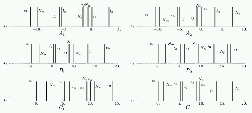
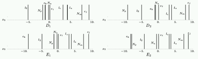
Figure 4: Complete field position configurations along the extra dimension (parameterized by $x_{5}$ in units of $\mu^{-1}$) associated to one point in each of the domains $A_{1,2},B_{1,2},C_{1,2},D_{1,2},E_{1,2}$ (see text) of parameter space $\{e,l,N,M_{R}\}$. The $e$ indices $\{i,j,k\}$ (distributed among $[1,2,3]$) and $l$ indices $\{a,c\}$ (distributed among $[1,3]$) obey to the same indice notation as the one adopted in Eq.(B.11). Thus, some of the distances, between $l$ and $e$ positions, shown here are given by Eq.(B.11). Similarly, the $N$ indices $\{m,n,p\}$ (distributed among $[1,2,3]$) correspond to the indices of Eq.(B.12), Eq.(B.13) and Eq.(B.14), so that the configurations of $l$ and $N$ presented here are quantified in those relations. Each point has been chosen in order to have $l_{2}$ given by the value associated to highest peak of its distribution (for the relevant domain).

\psfrag{l1}[c][c][1]{$l_{1}$}\psfrag{l2}[c][c][1]{$l_{2}$}\includegraphics[height=113.81102pt,width=216.81pt]{l1l2B1.eps}	\psfrag{l1}[c][c][1]{$l_{1}$}\psfrag{N1}[c][c][1]{$N_{1}$}\includegraphics[height=113.81102pt,width=216.81pt]{N1l1B1.eps}
\psfrag{N1}[c][c][1]{$N_{1}$}\psfrag{N2}[c][c][1]{$N_{2}$}\includegraphics[height=113.81102pt,width=216.81pt]{N1N2B1.eps}	\psfrag{N1}[c][c][1]{$N_{1}$}\psfrag{N3}[c][c][1]{$N_{3}$}\includegraphics[height=113.81102pt,width=216.81pt]{N1N3B1.eps}

Figure 5: Fundamental parameters $l_{1,2}$ and $N_{1,2,3}$ (units of $\mu^{-1}$) in the domain $B_{1}$ (see text) for which $0=e_{1}\simeq l_{3}-\mu^{-1}\sqrt{-2\ln(m^{exp}_{e^{\pm}}/\rho)}$, $e_{2}\simeq l_{1}+\mu^{-1}\sqrt{-2\ln(m^{exp}_{\tau^{\pm}}/\rho)}$, $e_{3}\simeq l_{2}+\mu^{-1}\sqrt{-2\ln(m^{exp}_{\mu^{\pm}}/\rho)}$ (we take $i=1$, $j=2$, $k=3$, $a=1$, $c=3$ in Eq.(B.11)), and, $N_{2}\approx{3l_{b}-l_{2}\over 2}$, $N_{1}\approx N_{3}\approx{l_{b}+l_{2}\over 2}$ (we choose $m=2$, $n=1$, $p=3$ in Eq.(B.12)).

In order to illustrate these results, we show explicitly, on Fig.(4), a given point in each of the 10 distinct regions $A_{i},B_{i},C_{i},D_{i},E_{i}\ [i=1,2]$ of parameter space $\{e_{i},l_{j},N_{k},M_{R}\}$. Furthermore, on Fig.(5), we present the entire region in $\{e_{i},l_{j},N_{k}\}$ associated to $B_{1}$.

Based on the physical interpretation of the 2 flavor case given in Section 3.2, we discuss now the various mixing angles associated to the obtained solutions $A_{i},B_{i},C_{i},D_{i},E_{i}\ [i=1,2]$.
Let us begin with an explanation of the two types of characteristic configurations (B.12) and (B.13) for positions $l_{i},N_{j}$. For simplification reasons, we take for instance $m=1$, $n=2$ and $p=3$ in both Eq.(B.12) and Eq.(B.13). Then, Eq.(B.13) can be rewritten as,

$$N_{1}\approx{3l_{1}-l_{2}\over 2},\ N_{2}\approx{l_{1}+l_{2}\over 2},$$ (107)

$$N_{2}\approx{l_{2}+l_{3}\over 2},\ N_{3}\approx{3l_{2}-l_{3}\over 2}.$$ (108)

These typical configurations (107) and (108) are equivalent to the configuration (33), with respectively $N_{1}$ and $N_{3}$ far from $N_{2}$ (see Fig.(1)[c,d]), which leads to a nearly maximum mixing in the neutrino sector within the context of 2 flavors. Hence, the configurations (107) and (108) give rise to the neutrino mixing angle values: $\theta_{12}^{\nu}\approx\pi/4$ and $\theta_{23}^{\nu}\approx\pi/4$. Indeed, the sectors $\nu_{e}-\nu_{\mu}$ and $\nu_{\mu}-\nu_{\tau}$ decouple from each other, due to a small value for $\theta_{13}^{\nu}$, and can thus be treated as separated 2 flavor sectors. More precisely, in Eq.(107) and Eq.(108), while the relation involving $N_{2}$ leads to $\theta_{12}^{\nu}\approx\pi/4$ and $\theta_{23}^{\nu}\approx\pi/4$ (like in Eq.(33)), the relations on $N_{1}$ and $N_{3}$ give rise to $\theta_{13}^{\nu}\approx 0$ as well as field positions compatible with the experimental neutrino mass squared differences.
Similarly, for $m=1$, $n=2$ and $p=3$, Eq.(B.12) can be rewritten:

$$N_{1}\approx{3l_{1}-l_{2}\over 2},\ N_{2}\approx{l_{1}+l_{2}\over 2},$$ (109)

$$N_{2}\approx{l_{2}+l_{3}\over 2},\ N_{3}\approx{l_{2}+l_{3}\over 2}.$$ (110)

The typical configuration (110) is identical to $N_{2}+N_{3}\approx l_{2}+l_{3}$ (see Eq.(34)), for $N_{2}\approx N_{3}$ (see Fig.(1)[c,d]), leading to a quasi maximal mixing in the neutrino sector if only 2 flavors are considered. As before, in Eq.(109) and Eq.(110), the relations involving $N_{2}$ and $N_{3}$ lead thus to $\theta_{12}^{\nu}\approx\pi/4$ and $\theta_{23}^{\nu}\approx\pi/4$, whereas the formula in which enters $N_{1}$ gives rise to $\theta_{13}^{\nu}\approx 0$ and allows the neutrino mass squared differences to have correct values.
To sum up, the characteristic 3 flavor configuration of $l_{i},N_{j}$ given by Eq.(B.12) is based on the two typical configurations (33) and (34) described in details in Section 3.2 and leading both to a quasi maximal mixing for the neutrino sector within a 2 flavor framework. In contrast, the typical 3 flavor configuration (B.13) is only based on the 2 flavor configuration (33) explained and interpreted in Section 3.2.
We conclude from this discussion that the parameters in regions $A_{i},B_{i},C_{i},D_{i},E_{i}\ [i=1,2]$, which obey to the relations (B.12) if $i=1$ and (B.13) if $i=2$, lead to $\theta_{12}^{\nu}\approx\pi/4$, $\theta_{23}^{\nu}\approx\pi/4$ and $\theta_{13}^{\nu}\approx 0$. Now, the solutions $A_{i},B_{i},C_{i},D_{i},E_{i}\ [i=1,2]$ reproduce the wanted values for the 3 mixing angles parameterizing $U_{MNS}$ (see Eq.(95)), namely $|\theta_{12}|\approx\pi/4$ (Eq.(102)), $|\theta_{23}|\approx\pi/4$ (Eq.(99)) and $\theta_{13}\approx 0$ (Eq.(96)). Therefore (see Eq.(31)), in the domains $A_{i},B_{i},C_{i},D_{i},E_{i}\ [i=1,2]$, the 3 mixing angles of charged lepton sector, which parameterize $U_{lL}$, are approximately equal to either $0$ or $\pi/2$. It means that there is an almost vanishing effective mixing in the charged lepton sector for the typical localization configurations of $e_{i},l_{j}$ (consistent with $m_{e^{\pm},\mu^{\pm},\tau^{\pm}}=m^{exp}_{e^{\pm},\mu^{\pm},\tau^{\pm}}$) given by Eq.(B.11) (classes of solutions described in Section 4.1), as we said in Section 4.1.

4.2.4 Conclusion

In summary of this section, we have found the less fine-tuned solutions in parameter space $\{e_{i},l_{j},N_{k}$, $M_{R}\}$ in agreement with all the present experimental data on charged lepton masses, neutrino mass squared differences and leptonic mixing angles (Eq.(96), Eq.(99) and Eq.(102)). These solutions can be classified into some of the different types of $e_{i},l_{j}$ configurations defined in Section 4.1, which correspond to a nearly vanishing effective mixing in the charged lepton sector. In fact, these solutions obey to the characteristic relations (B.12) or (B.13) on field positions $l_{j},N_{k}$, leading both to neutrino mixing angles responsible for almost the whole leptonic mixing observed experimentally. We have explained and interpreted those final solutions, and we have presented (description in Appendix B together with Fig.(4)) all the associated regions of parameter space $\{e_{i},l_{j},N_{k}$,$M_{R}\}$ ($A_{1,2},B_{1,2},C_{1,2},D_{1,2},E_{1,2}$), except the ranges of values for the typical Majorana mass scale $M_{R}$ that we will give and discuss in Section 5.

4.3 Discussion

4.3.1 Fine-tuning

We estimate here the variation ratio of type (46) for the different parameters in domain $B_{1}$ (see Section 4.2), for example. Remind that the solution $B_{1}$ reproduces all the present experimental data on leptonic sector: the experimental values for $m^{exp}_{e^{\pm},\mu^{\pm},\tau^{\pm}}$ and the constraints of Eq.(96), Eq.(99) and Eq.(102). As in Fig.(5), we consider the domain $B_{1}$ characterized by $i=1$, $j=2$, $k=3$, $a=1$, $c=3$ (see Eq.(B.11)) and $m=2$, $n=1$, $p=3$ (see Eq.(B.12)). The largest quantities (46) are the following ones. From Eq.(B.11), we obtain an analytical expression for the partial derivative of $m_{\tau^{\pm}}$ relatively to $e_{2}$, from which we deduce,

$$\bigg{|}{\delta\ln m_{\tau^{\pm}}\over\delta\ln e_{2}}\bigg{|}=-2\ln(m^{exp}_{\tau^{\pm}}/\rho)\simeq 10.$$ (111)

Similarly, Eq.(B.11) leads to,

$$\bigg{|}{\delta\ln m_{\mu^{\pm}}\over\delta\ln e_{3}}\bigg{|}=-2\ln(m^{exp}_{\mu^{\pm}}/\rho)\simeq 16,\ \bigg{|}{\delta\ln m_{e^{\pm}}\over\delta\ln l_{3}}\bigg{|}=-2\ln(m^{exp}_{e^{\pm}}/\rho)\simeq 26.$$ (112)

Within the region $B_{1}$, and for the smallest $N_{1}$ values, the quantity $\delta\ln X_{i}$, where $X_{i}=\{l_{1},l_{2},N_{1},N_{2},N_{3}\}$, is about $\delta\ln X_{i}\sim 10^{-1}$, as illustrated by Fig.(5). Hence, based on Eq.(96), Eq.(99) and Eq.(102), we find,

$$\bigg{|}{\delta\ln(\sin\theta_{13})\over\delta\ln X_{i}}\bigg{|}\simeq 20,\ \bigg{|}{\delta\ln(\tan^{2}\theta_{23})\over\delta\ln X_{i}}\bigg{|}\simeq 16,\ \bigg{|}{\delta\ln(\tan^{2}\theta_{12})\over\delta\ln X_{i}}\bigg{|}\simeq 12,$$ (113)

$$\bigg{|}{\delta\ln(\Delta m^{2}_{23})\over\delta\ln X_{i}}\bigg{|}\simeq 9,\ \bigg{|}{\delta\ln(\Delta m^{2}_{12})\over\delta\ln X_{i}}\bigg{|}\simeq 14.$$ (114)

Finally, in the part of $B_{1}$ where the $N_{1}$ values are minimum, one has $10^{4}{\rm GeV}\lesssim M_{R}\lesssim 10^{12}{\rm GeV}$ and the variation of $M_{R}$ (entire width of interval (106)), associated to the variations of $\Delta m^{2}_{23}$ and $\Delta m^{2}_{12}$ within their respective experimental range, reads as $\delta\ln M_{R}\simeq 0.43$. We thus find (see Eq.(99) and Eq.(102)),

$$\bigg{|}{\delta\ln(\Delta m^{2}_{23})\over\delta\ln M_{R}}\bigg{|}\simeq 2,\ \bigg{|}{\delta\ln(\Delta m^{2}_{12})\over\delta\ln M_{R}}\bigg{|}\simeq 3.$$ (115)

4.3.2 Perturbative bound

Let us make here a fundamental comment concerning the quantity $\Delta X_{MAX}$ (introduced in Section 3.4), namely the largest difference $|X_{i}-X_{j}|$ where $X_{i,j}=\{e_{1,2,3},l_{1,2,3},N_{1,2,3}\}$. Inside the whole domains of parameter space obtained ($A_{1,2},B_{1,2},C_{1,2},D_{1,2},E_{1,2}$), which fit all the present experimental data on leptonic sector, one has systematically,

$$15\mu^{-1}\lesssim\Delta X_{MAX}\lesssim 30\mu^{-1},$$ (116)

as can be deduced from Eq.(B.11), Eq.(B.12), Eq.(B.13), Eq.(B.15) and Eq.(B.17). This result on $\Delta X_{MAX}$ can be clearly seen in Fig.(5), for the example of entire region $B_{1}$. By consequence (since $\Delta X_{MAX}\lesssim L$), for all our final solutions in parameter space $\{e_{1,2,3},l_{1,2,3},N_{1,2,3},M_{R}\}$, the important constraint on wall thickness $L\lesssim 30\mu^{-1}$ (see Eq.(14)), coming from considerations concerning perturbativity, can be well respected.

We end up this part by noting that the less fine-tuned consistent realizations of the AS scenario, that we obtain (regions $A_{1,2},B_{1,2},C_{1,2},D_{1,2},E_{1,2}$ of parameter space), do not recover the particular field localization configuration proposed in [30] for justifying a minimal see-saw model.

5 Predictions

In this part, we will describe some features and predictions for neutrino sector, within the see-saw model, which are provided by the complete and consistent realizations of AS scenario obtained in Section 4.2. We will have a look on the light left-handed neutrino sector and then on the heavy right-handed one. Our solutions are quite predictive on the mixing angle $\theta_{13}$ and lead to a more precise prediction on the lightest neutrino mass eigenvalue $m_{\nu_{1}}$. So we will compare our predictions on those two physical quantities with the corresponding present and future neutrino experiment sensitivities. We will finish by important comments on the value of parameter $\rho$.

We will first consider the case of normal hierarchy for light left-handed neutrino masses (as before), and the inverted hierarchy case will be discussed after in a separate section.

5.1 Normal Mass Hierarchy

\psfrag{m1}[c][c][1]{{\myblue$m_{\nu_{1}}$}}\psfrag{m2}[c][c][1]{{\mygreen$m_{\nu_{2}}$}}\psfrag{m3}[c][c][1]{{\myred$m_{\nu_{3}}$}}\psfrag{lmi}[c][r][1][90]{$Log_{10}[m_{\nu_{i}}\ {\rm(eV)}]$}\psfrag{logMGeV}[c][r][1]{$Log_{10}[M_{R}\ {\rm({\rm GeV})}]$}\includegraphics[width=216.81pt,height=142.26378pt]{miM.eps}	\psfrag{myF1}[c][c][1][90]{$m_{\nu_{1}}\ ({\rm eV})$}\psfrag{m1max}[c][c][1]{{\scriptsize{\myblue$m^{min}_{\nu_{1}}$}}}\psfrag{m1min}[c][c][1]{{\scriptsize{\mygreen$m^{max}_{\nu_{1}}$}}}\psfrag{LogMGeV}[c][r][1]{$Log_{10}[M_{R}\ {\rm(GeV)}]$}\includegraphics[width=216.81pt,height=142.26378pt]{m1rangeM.eps}
[a]	[b]

Figure 6: Light neutrino masses $m_{\nu_{1}}$, $m_{\nu_{2}}$ and $m_{\nu_{3}}$ (eV) [a] and boundaries of the allowed range for $m_{\nu_{1}}$ (eV) [b] as a function of right-handed Majorana neutrino mass $M_{R}$ (GeV). The $m_{\nu_{i}}$ values in [a] correspond to the lower limit of allowed mass range (in particular, $m_{\nu_{1}}$ in [a] corresponds to $m_{\nu_{1}}^{min}$ in [b]). The values shown in [a] and [b] correspond to the solutions $A,B,C,D,E|_{1,2}$ defined in Appendix B.

5.1.1 Light left-handed sector

The $M_{R}$ values being given by the range (106), we derive from Eq.(30) the ground of light neutrino masses $m_{\nu_{1}}$, i.e. the corresponding range for the lightest neutrino: $m_{\nu_{1}}\in[m^{min}_{\nu_{1}},m_{\nu_{1}}^{max}]$, where,

$$m_{\nu_{1}}^{max}=INF\left(\sqrt{\Delta m^{2}_{12max}}{V_{1}\over\sqrt{V^{2}_{2}-V_{1}^{2}}}\ ,\ \sqrt{\Delta m^{2}_{23max}}{V_{1}\over\sqrt{V^{2}_{3}-V_{2}^{2}}}\right),$$ (117)

and,

$$m_{\nu_{1}}^{min}=SUP\left(\sqrt{\Delta m^{2}_{12min}}{V_{1}\over\sqrt{V^{2}_{2}-V_{1}^{2}}}\ ,\ \sqrt{\Delta m^{2}_{23min}}{V_{1}\over\sqrt{V^{2}_{3}-V_{2}^{2}}}\right).$$ (118)

Our solutions exhibit a quite remarkable feature. Indeed, for all our final models, though running together over several orders of magnitude, $V_{1}$, $V_{2}$ and $V_{3}$ remain actually of the same order and such that the ratios $V_{1}/\sqrt{V^{2}_{2}-V_{1}^{2}}$ and $V_{1}/\sqrt{V^{2}_{3}-V_{2}^{2}}$ are close to one, leading to nearly constant bounds $m^{min}_{\nu_{1}}$ and $m^{max}_{\nu_{1}}$. Furthermore, those two bounds are systematically close, which gives rise to the generic prediction:

$$m_{\nu_{1}}\sim 10^{-2}{\rm eV},$$

and consequently to the typical spectrum:

$$m_{\nu_{1}}\sim m_{\nu_{2}}\lesssim m_{\nu_{3}}.$$

This picture is illustrated on Fig.(6). A more physical way to understand the constance of $m_{\nu_{1}}$ in our solutions is the following: there is a compensation in Eq.(30) between the variations of $M_{R}$ (entering the suppression factor $\rho/M_{R}$ due to the see-saw mechanism) and $V_{i}$ (depending on the suppression factors issued from wave function overlaps).

Besides, our solutions correspond to $0.05{\rm eV}<\sum m_{i}<0.12{\rm eV}$ which agrees with the upper cosmological bound $\sum m_{i}<0.7-1.01{\rm eV}$ (depending on cosmological priors) coming from WMAP and 2dFGRS galaxy survey [39].

5.1.2 Heavy right-handed sector

Lepton masses and mixings fix the positions $\{e_{i},l_{j},N_{k}\}$ accordingly to configurations such that $N_{1},N_{2}$ and $N_{3}$ are quite far from each other (see Fig.(4)). This leads to a quasi diagonal Majorana mass matrix $M_{ij}$ (Eq.(11)), up to essentially one non-diagonal term $M_{np}$ ($n$ and $p$ correspond to the $N$ indices in Fig.(4)) which can reach $\sim 0.5M_{R}$ in solutions $A,B,C,D,E|_{1}$. This texture gives rise to three eigenvalues $M_{i}$, for the Majorana mass matrix $M_{ij}$ (Eq.(11)), of the same order of magnitude:

$$M_{1}\sim M_{2}\sim M_{3}\sim M_{R},$$

especially in the second type of solutions $A,B,C,D,E|_{2}$ where, $|N_{n}-N_{p}|$ being higher (see Fig.4), one has an almost exact degeneracy. This is illustrated on Fig.(7)[a].

\psfrag{M1}[c][c][1]{{\myblue$M_{1}$}}\psfrag{M2}[c][c][1]{{\mygreen$M_{2}$}}\psfrag{M3}[c][c][1]{{\myred$M_{3}$}}\psfrag{lMi}[c][r][1][90]{$Log_{10}[M_{i}\ {\rm(GeV)}]$}\psfrag{logMGeV}[c][r][1]{$Log_{10}[M_{R}\ {\rm(GeV)}]$}\includegraphics[width=216.81pt,height=142.26378pt]{MiM.eps}	\psfrag{ABCDE1}[c][r][1][1]{\scriptsize{{\myblue$A,B,C,D,E|_{1}$}}}\psfrag{ABCDE2}[c][r][1][1]{\scriptsize{{\myred$A,B,C,D,E|_{2}$}}}\psfrag{l1N3}[c][r][1][90]{$|l_{1}-N_{3}|\ (\mu^{-1})$}\psfrag{logMGeV}[c][r][1]{$Log_{10}[M_{R}\ {\rm(GeV)}]$}\includegraphics[width=216.81pt,height=142.26378pt]{l1N3M.eps}
[a]	[b]

Figure 7: [a] Right-handed neutrino masses $M_{1},M_{2},M_{3}$ (GeV) as function of the common scale $M_{R}$ (GeV) (Eq.(11)). [b] Correlation of $M_{R}$ with the field position difference $|l_{1}-N_{3}|$ (in units of $\mu^{-1}$). The values shown in [a] and [b] correspond to the solutions $A,B,C,D,E|_{1,2}$ defined in Appendix B.

Let us now discuss the $M_{R}$ values associated to all our solutions. We have chosen to present in Fig.(6) and Fig.(7) the $M_{R}$ values corresponding to the upper boundary of allowed range (106), the two boundaries being actually close ($0.65<{\rm ratio}<1$) for each point of our solutions. When field positions vary, due to the presence of exponential factors, the eigenvalues $V_{i}$ vary strongly so that $M_{R}$ spans several orders of magnitude (see Eq.(106)). As we want to stay in the see-saw mechanism spirit, we impose as a minimum $M_{R}\gtrsim 10^{2}{\rm GeV}$, which explains the lower $M_{R}$ axis boundary on Fig.(6) and Fig.(7).
In contrast, the upper bound appearing on Fig.(6) and Fig.(7), namely:

$$M_{R}\lesssim 10^{12}{\rm GeV},$$

is a consequence of the localization configurations we have obtained. Let us try to understand this bound. Due to the small value of mixing angle $\theta_{13}$, the sectors $\nu_{e}-\nu_{\mu}$ and $\nu_{\mu}-\nu_{\tau}$ decouple. Hence, we deduce from the discussion within the 2 lepton flavor case (end of Section 3.3) that the quantities $M^{max}_{R12}$ (defined in Eq.(104)) and $M^{max}_{R23}$ (defined in Eq.(105)) satisfy to $M^{max}_{R12}\lesssim 10^{16}{\rm GeV}$ and $M^{max}_{R23}\lesssim 10^{15}{\rm GeV}$ (see Eq.(45)). Nevertheless, $M^{max}_{R12}$ and $M^{max}_{R23}$ do not reach their upper value in the same region of parameter space $\{e_{i},l_{j},N_{k}\}$ (otherwise Eq.(106) would lead to $M_{R}<INF(M^{max}_{R12},M^{max}_{R23})\lesssim INF(10^{16}{\rm GeV},10^{15}{\rm GeV})=10^{15}{\rm GeV}$) which explains why the resulting upper limit on $M_{R}$, namely $\sim 10^{12}{\rm GeV}$, is smaller than $\sim 10^{15}{\rm GeV}$.
Why the upper limit on $M_{R}$ is higher for solutions $A,B,C,D,E|_{1}$ than $A,B,C,D,E|_{2}$ ? In solutions of type 1, the position difference $|l_{b}-N_{p}|$ [$b=1,3$] is systematically smaller than in configurations of type 2, as it is clear on Fig.(4). Therefore, the eigenvalues $V_{i}$ are typically larger in solutions of type 1 than in solutions of type 2. The consequence (see Eq.(106)) is that $M_{R}$ can reach larger values in solutions of type 1. This argument is illustrated in Fig.(3)[b] for the case: $b=1$ and $p=3$.

Finally, our result of three right-handed Majorana masses remaining of the same order, over ten orders of magnitude, is interesting with regard to the leptogenesis. We postpone leptogenesis, in this AS framework based on the see-saw mechanism, for a next coming paper [40].

5.1.3 Comparison with experimental sensitivities

Today, there are still two measurable quantities (forgetting relevant phases) undetermined (actually weakly constrained), in the light neutrino sector: the ground of neutrino masses (namely $m_{\nu_{1}}$, in the normal hierarchy case with our conventions) and the mixing angle $\theta_{13}$. For those two physical quantities, we are going to briefly remind the experimental status and then compare the experimental sensitivities with our predictions.

Concerning the lightest neutrino mass, the present measurements of kinematics in tritium $\beta$ decay give rise to the bound $m_{\nu_{1}}<2.2{\rm eV}$ (Mainz [43] and Troisk [44] Collaborations). This result will be improved by the KATRIN project [45] down to $m_{\nu_{1}}<0.35{\rm eV}$.
Furthermore, neutrinoless double $\beta$ decay (see [46] for a recent review) experiments are sensitive to the so-called effective neutrino mass: $m_{ee}=|\sum_{i}U^{2}_{ei}m_{\nu_{i}}|$ ($U_{ei}$ are the first line elements of $U_{MNS}$ matrix (95)). Those measurements are complementary with those on $m_{\nu_{1}}$ because they require neutrinos to be Majorana particles. The Heidelberg-Moscow experiment [47] obtains the lowest limit: $m_{ee}<0.35{\rm eV}$. This bound will be improved by next generation experiments like EXO [48], MOON [49], XMASS [50], NEMO3 [51], CUORE [52] and GENIUS [53], down to $m_{ee}\lesssim 10^{-2}{\rm eV}$ (highest expected sensitivity) for the latter.

Concerning the $\theta_{13}$ mixing angle, $s_{13}$ (same notation as in Eq.(95)) is up to now constrained by the CHOOZ experiment [38]. For the $\Delta m^{2}_{13}$ value that we obtain: $\sqrt{\Delta m^{2}_{13}}\sim 5\ 10^{-2}{\rm eV}$ (see Fig.(6)), the bound from CHOOZ experiment is approximately $s_{13}<0.18$ [38], as we have imposed in our analysis (see Eq.(96)). This bound on $s_{13}$ will be improved (see e.g. [54, 55]) by superbeams like CNGS [56], JHF [57] and neutrino factories [58]. Depending on possible improvement, JHF-SK, JHF-HK (or low luminosity neutrino factories which have quite similar performances on $s_{13}$ measurement) and finally high luminosity neutrino factories will at least improve the bound down to respectively [54]: $s_{13}\lesssim 7\ 10^{-2}$, $1.6\ 10^{-2}$, $1.1\ 10^{-2}$.

\psfrag{se3}[c][r][1]{$s_{13}$}\psfrag{logm1eV}[c][r][1]{$Log_{10}[m_{\nu_{1}}\ {\rm(eV)}]$}\psfrag{katrin}[c][c][1]{{\scriptsize KATRIN}}\psfrag{mainz}[c][c][1]{{\scriptsize Mainz,}}\psfrag{troisk}[c][ct][1]{{\scriptsize Troisk}}\psfrag{JHF}[l][l][1]{{\scriptsize JHF-SK}}\psfrag{nuF}[l][l][1]{{\scriptsize$\nu$F2}}\includegraphics[width=216.81pt,height=142.26378pt]{m1se3.eps}

\psfrag{C}[l][l][1]{{\scriptsize CHOOZ}}\psfrag{J}[l][l][1]{{\scriptsize JHF-SK}}\psfrag{J2}[l][l][1]{{\scriptsize JHF-HK/$\nu$F1}}\psfrag{nuF}[l][l][1]{{\scriptsize$\nu$F2}}\psfrag{H}[l][l][1]{{\scriptsize Heidel}}\psfrag{N3}[l][l][1]{{\scriptsize NEMO3}}\psfrag{G}[l][l][1]{{\scriptsize GENIUS}}\psfrag{lse3}[c][r][1][90]{$Log_{10}[s_{13}]$}\psfrag{logmeeeV}[c][r][1]{$Log_{10}[m_{ee}\ {\rm(eV)}]$}\psfrag{-2.1}[c][r][1]{}\psfrag{-1.9}[c][r][1]{}\psfrag{-1.7}[c][r][1]{}\psfrag{-1.5}[c][r][1]{}\includegraphics[width=216.81pt,height=142.26378pt]{meese3manip.eps}

[a]

[b]

Figure 8: [a] $(m_{\nu_{1}},s_{13})$ plane with present (Mainz and Troisk) and future (KATRIN) experimental sensitivities on $m_{\nu_{1}}$. [b] $(m_{ee},s_{13})$ plane with current (Heidelberg) and future (NEMO3, GENIUS) bounds on $m_{ee}$ from double $\beta$ decay experiments. Current (CHOOZ) and future superbeams (JHF-SK, JHF-HK) and neutrino factories (low luminosity: $\nu$F1, high luminosity: $\nu$F2) sensitivities on $s_{13}$ are also represented. The values shown in [a,b] correspond to the solutions $A,B,C,D,E|_{1,2}$ and to the lower limit of neutrino mass interval (for instance, the $m_{\nu_{1}}$ value is taken equal to $m_{\nu_{1}}^{min}$).

All those sensitivities are indicated on Fig.(8) where we also show all our solutions: $A,B,C,$ $D,E|_{1,2}$ in the planes $(s_{13},m_{\nu_{1}})$ and $(s_{13},m_{ee})$. Our models are not extremely predictive on $s_{13}$ although they “prefer” the range:

$$10^{-2}\lesssim s_{13}\lesssim 10^{-1},$$

to which belongs most of our final solutions. It is interesting to remark that this range contains the best-fit value $s_{13}\simeq 0.1$ obtained in the global three neutrino oscillation analysis of [27]. Furthermore, this favored range will be directly tested by JHF-SK(HK) and neutrino factories. Concerning the masses, the relatively precise prediction on $m_{\nu_{1}}$ and $m_{ee}$, in the AS scenario based on the see-saw mechanism, is particularly clear on Fig.(8). The predicted value of $m_{\nu_{1}}$ is out of reach of Mainz and Troisk current bound and will not be reached by the future Katrin sensitivity (Fig.(8)[a]). Nevertheless, assuming zero-phases in $m_{ee}$ (our $U_{ei}$ being real), our solutions lead to the value $m_{ee}\sim 10^{-2}{\rm eV}$ which will be accessible by some future double $\beta$ decay experiments. Indeed, the GENIUS experiment should be able to test a wide set of our solutions, as shown in Fig.(8)[b]. Hence, future measurements on $\theta_{13}$ and $m_{\nu_{1}}$ will allow to either motivate or exclude most of our theoretical models.

5.1.4 Choice of the $\rho$ value

As explained in Section 3.1, within the considered AS scenario, the parameter $\rho=\kappa(m_{top})\langle h\rangle$ (defined in Eq.(6)) must be of the order of magnitude of the electroweak scale, since one should have $\kappa(m_{top})\approx 1$. Hence, one could assume an exact $\rho$ value a bit different from the one we have chosen, namely $\rho=1.5m_{top}(m_{top})$ (see Eq.(24)), as long as $\rho$ remains of the same order of magnitude of the electroweak scale. The important message that we deliver here is that such a different choice of $\rho$ would not have significantly affected our predictions on neutrino sector (both in the normal and inverted mass hierarchy cases).

As it is clear from Eq.(106), a modification of $\rho$ leads to a variation of $M_{R}$. Nevertheless, for a small modification of $\rho$ (such that $\rho$ remains of the order of electroweak scale), the $M_{R}$ values do not vary significantly.

Besides, within the present framework, the variations of left-handed neutrino masses $m_{\nu_{i}}=m_{\nu_{i}}(l_{j},N_{k})$ (given by Eq.(117) and Eq.(118)), due to a modification of $\rho$, would only originate from the variations of $V_{i}(l_{j},N_{k})$ eigenvalues (defined in Eq.(30)). Indeed, the obtained values of parameter $l_{j}$ (and $e_{i}$), and thus of $V_{i}(l_{j},N_{k})$, depend on $\rho$ (see Eq.(6)).
We find numerically that for a small modification of $\rho$ ($\rho$ staying around the order of magnitude of electroweak scale), the variations of all neutrino masses $m_{\nu_{i}}(l_{j},N_{k})$ are negligible. It is due to the fact that the constraints on parameters $l_{j},N_{k}$ (and $e_{i}$), issued from requiring lepton mixing angles compatible with their experimental bounds, are exactly invariant under a modification of $\rho$.

5.2 Inverted Mass Hierarchy

Here, we discuss the inverted hierarchy case which is characterized by:

$$m_{\nu_{3}}<m_{\nu_{2}}<m_{\nu_{1}},$$

with $\Delta m^{2}_{23}=m_{\nu_{2}}^{2}-m_{\nu_{3}}^{2}$ given by atmospheric neutrino oscillation data, and, $\Delta m^{2}_{12}=m_{\nu_{1}}^{2}-m_{\nu_{2}}^{2}$ given by solar neutrino oscillation data. For this neutrino mass hierarchy, our models lead to the same picture for $s_{13}$ and again three left-handed neutrino masses quite close to each other. However, this time the prediction is on $m_{\nu_{3}}$ (with the above notation):

$$m_{\nu_{3}}\sim 10^{-2}{\rm eV},$$

with the following spectrum:

$$\ m_{\nu_{3}}\lesssim m_{\nu_{1}}\sim m_{\nu_{2}}.$$

In the right-handed sector, the picture of three heavy masses of the same order of magnitude, namely $M_{i}\sim M_{R}$, is unchanged. Furthermore, due to the suppression of $m_{\nu_{3}}$ by $U_{e3}^{2}$ (small $s_{13}$ value) in the $m_{ee}$ expression, $m_{ee}$ is a bit higher in the inverted hierarchy case than in the normal hierarchy case. The cloud of our solutions would thus be centered on $m_{ee}\sim 4\ 10^{-2}{\rm eV}$ in the inverted hierarchy case (instead of $m_{ee}\sim 10^{-2}{\rm eV}$ as in the normal hierarchy case of Fig.(8)[b]), which implies that the GENIUS experiment would be able to test almost all our solutions.

6 Conclusion

We have studied the structure of lepton flavor space in the framework of the AS scenario with an extra dimension, under the assumption that neutrinos acquire Majorana masses via the see-saw mechanism.
First, we have given a generic description of the AS models reproducing the correct charged lepton masses and corresponding to a minimal fine-tuning of parameters. Then, we have shown that one can construct realistic AS models, namely compatible with all the present experimental data on the entire leptonic sector (charged lepton masses, and, constraints on mixing angles and neutrino masses), in which neutrinos acquire masses through the see-saw mechanism. We have found the realistic AS models of this kind giving rise to a minimum fine-tuning of the fundamental parameters (lepton field positions and neutrino Majorana mass scale $M_{R}$). Those AS models can be classified into some of the different types of localization configurations defined in Section 4.1, and, verify either the characteristic relation (B.12) or (B.13). Furthermore, all these AS models, which have been explained and interpreted, lead to neutrino mixing angles responsible for almost the whole effective leptonic mixing measured experimentally.

We have found that, within the considered AS framework based on the see-saw mechanism, the minimal fine-tuning on parameters (reached when examining all the relevant parameter space) is weaker than in the AS scenario where neutrinos acquire Dirac masses [24]. This is due to the fact that the parameters of our model are those of the AS scenario with neutrino Dirac masses (lepton field positions) plus an additional parameter ($M_{R}$). In the AS scenario with neutrino Dirac masses, there is an important fine-tuning of parameters, which can be considered as not acceptable [24]. In contrast, we have shown that some of our final solutions associated to the see-saw model (as for instance $B_{1}$), fitting all the experimental results on charged leptons and neutrinos, correspond to an acceptable fine-tuning of parameters. It means that, if nature has chosen the AS scenario in order to generate the whole lepton flavor structure, the case in which neutrino masses are produced via the see-saw mechanism seems to be the most favored one, as it can lead to a reasonable fine-tuning of parameters.

Moreover, we have demonstrated that, in the AS scenarios based on see-saw model that we have obtained, for $M_{R}$ values much greater than the electroweak symmetry breaking scale, the lepton field positions can be significantly closer to each other than in the whole parameter space of AS scenarios with neutrino Dirac masses [24]. In other terms, the see-saw mechanism is in favor of the naturality of the AS scenario, in the sense given in Section 1. Besides, we have obtained the important result that, even when considering the entire leptonic sector, the constraint on domain wall thickness along the extra dimension: $L\lesssim 30\mu^{-1}$, coming from considerations concerning perturbativity, can be well respected in concrete realizations of the AS scenario based on the see-saw model (as it occurs in all our final solutions).

One of our major quantitative results is the following one. The less fine-tuned realistic AS models based on the see-saw mechanism, that we have obtained, give rise to predictions on the whole neutrino sector. Indeed, our final models lead to three right-handed neutrino Majorana masses of the same order of magnitude:

$$M_{1}\sim M_{2}\sim M_{3}\sim M_{R},$$

and which can run between $\sim 10^{2}{\rm GeV}$ and $\sim 10^{12}{\rm GeV}$. Moreover, those models predict a ground level for left-handed neutrino Majorana masses, leading to the following typical mass spectrum,

$$m_{\nu_{1}}\sim m_{\nu_{2}}\sim 10^{-2}{\rm eV}<m_{\nu_{3}}\sim 5\ 10^{-2}{\rm eV} \quad{\rm[normal\ hierarchy]},$$

$$m_{\nu_{3}}\sim 10^{-2}{\rm eV}<m_{\nu_{2}}\sim m_{\nu_{1}}\sim 5\ 10^{-2}{\rm eV} \quad{\rm[inverted\ hierarchy]}.$$

Most of the values found for the effective neutrino mass $m_{ee}$, which correspond to this predicted spectrum, should be testable in future double $\beta$ decay experiments. Finally, our AS models favor the range of $\theta_{13}$ mixing angle value defined by,

$$10^{-2}\lesssim s_{13}\lesssim 10^{-1},$$

which should be accessible by future superbeam and neutrino factory sensitivities.

In fact, the concrete realization of AS scenario based on the see-saw mechanism that we have elaborated, together with the AS model in [23] which fits all quark masses and mixing angles, constitute the first realistic and complete realization of the AS scenario with one extra dimension. A complete realization in the sense that it reproduces all the present experimental data on SM fermions, and a realistic one in the three following senses. First, this realistic realization allows a reasonable fine-tuning of parameters. Secondly, in this realization, the experimental bounds on proton lifetime and FCNC rates are well respected. These bounds are satisfied thanks to the existence of large mass scales (see Section 2.3), which is possible as we have assumed that the fundamental energy scale is high ($M_{\star}^{5D}\gtrsim 10^{16}{\rm GeV}$). Thirdly, in this physical realization, the width of $x_{5}$ interval along the extra dimension, inside which all lepton (quark) fields are localized, ranges approximately between $15\mu^{-1}$ ($20\mu^{-1}$) and $30\mu^{-1}$ ($25\mu^{-1}$), as shown in our relation (116) (in [23]). Therefore, if both the lepton and quark fields are trapped in the same region of extra dimension, then the perturbativity condition on domain wall thickness $L\lesssim 30\mu^{-1}$ can be fulfilled.

How the hypothesis of a fundamental scale smaller than the GUT scale would have modify our study ? For $M_{\star}^{5D}\lesssim 10^{16}{\rm GeV}$, the interactions mediating proton decay (and FCNC reactions) should be partially suppressed through a localization of quarks and leptons (and SM fermions of different families) at far positions from each other, the suppression due to large mass scales being not sufficient (see Section 2.3). For instance, if $M_{\star}^{5D}\sim 1{\rm TeV}$, the proton can be stable enough, for a distance between quark and lepton positions in the extra dimension of at least $\sim 10\mu^{-1}$ [13]. Those lower bounds on distances between field positions make that the perturbativity condition on domain wall width $L\lesssim 30\mu^{-1}$ is not necessarily (or easily) satisfied when one considers all the SM fermions, depending on the $M_{\star}^{5D}$ value and localization configuration. In particular, the FCNC constraints on field positions could even be not compatible with the experimental data on SM fermions.

Finally, let us comment on the other hierarchy problem in the SM: the instability of the Higgs boson mass, and thus the electroweak energy scale, with respect to quantum corrections. In a reasonable realization of the AS scenario with only one extra dimension, this hierarchy problem does not seem to be able to be solved by bringing the Planck scale down to just above the electroweak scale (as proposed in [2]). Indeed, as discussed previously, in complete realistic AS models with one extra dimension, the width of $x_{5}$ range, in which all fields are localized, must be larger than at least $\sim 10\mu^{-1}$ typically (for instance, in the quark model of [23], it is larger than $\sim 20\mu^{-1}$), so that one has $L\gtrsim 10\mu^{-1}$. Now, this bound on $L$ together with the constraint characteristic of the AS scenario, $\mu^{2}L<M_{\star}^{5D}$ (see Section 2.3), imply the typical limit on fundamental scale: $M_{\star}^{5D}\gtrsim 100L^{-1}\gtrsim 100{\rm TeV}$, as $L^{-1}$ cannot be pushed significantly below roughly $1{\rm TeV}$. Nevertheless, one could try to find a particular realization of AS scenario with more than one extra dimension, which would allow to greatly reduce the $M_{\star}^{5D}$ value. Anyway, if the hierarchy problem of Higgs mass instability is solved by bringing the Planck scale down to $M_{\star}^{5D}={\cal O}(1){\rm TeV}$, then the motivation for the see-saw model becomes weaker. As a matter fact, in such a situation, the Majorana mass scale is bounded by $M_{R}\lesssim 1{\rm TeV}$, so that the see-saw mechanism cannot be responsible for a significant suppression of left-handed neutrino masses relatively to the electroweak scale ($\rho$: see Eq.(12)) and looses thus its important rôle with regard to neutrino mass generation. Therefore, in realizations of the AS scenario, based on the see-saw mechanism, it is desirable that the hierarchy problem can be solved by a model compatible with a $M_{\star}^{5D}$ value larger than the electroweak scale. For example, the Higgs mass can be stabilized in a supersymmetric theory softly broken at the electroweak scale, because of the cancellation of all quadratically divergent quantum corrections.

Acknowledgments

The authors are grateful to P. Aliani, M. V. Libanov and J. Orloff for interesting discussions. G. M. and E. N. acknowledge support from the Belgian Federal Government under contract IAP V/27, the French Community of Belgium (ARC) and the IISN.

Appendix

Appendix A Neutrino Mass Matrix Expression

In the case of two lepton flavors ($\{i,j\}=2,3$), the expression for left-handed neutrino mass matrix generated by the see-saw mechanism within an AS context (namely the Majorana mass matrix of Eq.(12)) reads as,

$$m^{\nu}_{ij}\simeq\left(\begin{array}[]{cc}m^{\nu}_{22}&m^{\nu}_{23}\\ m^{\nu}_{23}&m^{\nu}_{33}\end{array}\right),\ \mbox{with},\$$

$$m^{\nu}_{22} = -{\rho^{2}\over M_{R}(1-e^{-\mu^{2}(N_{2}-N_{3})^{2}})}\bigg{(}e^{-\mu^{2}(l_{2}-N_{2})^{2}}+e^{-\mu^{2}(l_{2}-N_{3})^{2}}$$ (A.2)

$$-2e^{-{\mu^{2}\over 2}[(N_{2}-N_{3})^{2}+(l_{2}-N_{2})^{2}+(l_{2}-N_{3})^{2}]}\bigg{)},$$

$$m^{\nu}_{33} = -{\rho^{2}\over M_{R}(1-e^{-\mu^{2}(N_{2}-N_{3})^{2}})}\bigg{(}e^{-\mu^{2}(l_{3}-N_{2})^{2}}+e^{-\mu^{2}(l_{3}-N_{3})^{2}}$$ (A.4)

$$-2e^{-{\mu^{2}\over 2}[(N_{2}-N_{3})^{2}+(l_{3}-N_{2})^{2}+(l_{3}-N_{3})^{2}]}\bigg{)},$$

$$m^{\nu}_{23} = -{\rho^{2}\over M_{R}(1-e^{-\mu^{2}(N_{2}-N_{3})^{2}})}\bigg{(}e^{-{\mu^{2}\over 2}[(l_{3}-N_{2})^{2}+(l_{2}-N_{2})^{2}]}+e^{-{\mu^{2}\over 2}[(l_{3}-N_{3})^{2}+(l_{2}-N_{3})^{2}]}$$ (A.6)

$$-e^{-{\mu^{2}\over 2}[(N_{2}-N_{3})^{2}+(l_{3}-N_{2})^{2}+(l_{2}-N_{3})^{2}]}-e^{-{\mu^{2}\over 2}[(N_{2}-N_{3})^{2}+(l_{2}-N_{2})^{2}+(l_{3}-N_{3})^{2}]}\bigg{)}.$$

Appendix B Final 3 Flavor Solutions

The less fine-tuned solutions in parameter space $\{e_{i},l_{j},N_{k},M_{R}\}$ fitting all the present experimental data on leptons ($m_{e^{\pm},\mu^{\pm},\tau^{\pm}}=m^{exp}_{e^{\pm},\mu^{\pm},\tau^{\pm}}$ together with the ranges of Eq.(96), Eq.(99) and Eq.(102)) constitute ten distinct and limited regions, that we denote as $A_{i},B_{i},C_{i},D_{i},E_{i}\ [i=1,2]$. In this appendix, we describe those regions in details.

First, the regions $A_{i},B_{i},C_{i},D_{i},E_{i}\ [i=1,2]$ correspond to some of the different types of localization configurations consistent with the experimental charged lepton masses described in Section 4.1. Indeed, the points in these domains have coordinates obeying to the following respective relations ($\{i,j,k\}$ are distributed among $[1,2,3]$, and, $\{a,c\}$ among $[1,3]$),

$$A_{1,2}:\ \ \ \ \ \ \ \ \ \ \ \ \ \ \ \ \ \ \ \ \ \ \ \ \ \ \ \ \ \ \ \ \ \ \ \ \ \ \ \ \ \ \ \ \ \ \ \ \ \ \ \ \ \ \ \ \ \ \ \ \ \ \ \ \ \ \ \ \ \ \ \ \ \ \ \ \ \ \ \ \ \ \ \ \ \ \ \ \ \ \ \ \ \ \ \ \ \ \ \ \ \ \ \ \ \ \ \ \ \ \ \ \ \ \ \ \$$ (B.1)

$$e_{i}\simeq l_{2}-\mu^{-1}\sqrt{-2\ln(m^{exp}_{\tau^{\pm}}/\rho)};e_{j}\simeq l_{c}+\mu^{-1}\sqrt{-2\ln(m^{exp}_{\mu^{\pm}}/\rho)};e_{k}\simeq l_{a}-\mu^{-1}\sqrt{-2\ln(m^{exp}_{e^{\pm}}/\rho)},$$ (B.2)

$$B_{1,2}:\ \ \ \ \ \ \ \ \ \ \ \ \ \ \ \ \ \ \ \ \ \ \ \ \ \ \ \ \ \ \ \ \ \ \ \ \ \ \ \ \ \ \ \ \ \ \ \ \ \ \ \ \ \ \ \ \ \ \ \ \ \ \ \ \ \ \ \ \ \ \ \ \ \ \ \ \ \ \ \ \ \ \ \ \ \ \ \ \ \ \ \ \ \ \ \ \ \ \ \ \ \ \ \ \ \ \ \ \ \ \ \ \ \ \ \ \$$ (B.3)

$$e_{i}\simeq l_{c}-\mu^{-1}\sqrt{-2\ln(m^{exp}_{e^{\pm}}/\rho)};e_{j}\simeq l_{a}+\mu^{-1}\sqrt{-2\ln(m^{exp}_{\tau^{\pm}}/\rho)};e_{k}\simeq l_{2}+\mu^{-1}\sqrt{-2\ln(m^{exp}_{\mu^{\pm}}/\rho)},$$ (B.4)

$$C_{1,2}:\ \ \ \ \ \ \ \ \ \ \ \ \ \ \ \ \ \ \ \ \ \ \ \ \ \ \ \ \ \ \ \ \ \ \ \ \ \ \ \ \ \ \ \ \ \ \ \ \ \ \ \ \ \ \ \ \ \ \ \ \ \ \ \ \ \ \ \ \ \ \ \ \ \ \ \ \ \ \ \ \ \ \ \ \ \ \ \ \ \ \ \ \ \ \ \ \ \ \ \ \ \ \ \ \ \ \ \ \ \ \ \ \ \ \ \ \$$ (B.5)

$$e_{i}\simeq l_{c}-\mu^{-1}\sqrt{-2\ln(m^{exp}_{e^{\pm}}/\rho)};e_{j}\simeq l_{a}+\mu^{-1}\sqrt{-2\ln(m^{exp}_{\tau^{\pm}}/\rho)};e_{k}\simeq l_{2}-\mu^{-1}\sqrt{-2\ln(m^{exp}_{\mu^{\pm}}/\rho)},$$ (B.6)

$$D_{1,2}:\ \ \ \ \ \ \ \ \ \ \ \ \ \ \ \ \ \ \ \ \ \ \ \ \ \ \ \ \ \ \ \ \ \ \ \ \ \ \ \ \ \ \ \ \ \ \ \ \ \ \ \ \ \ \ \ \ \ \ \ \ \ \ \ \ \ \ \ \ \ \ \ \ \ \ \ \ \ \ \ \ \ \ \ \ \ \ \ \ \ \ \ \ \ \ \ \ \ \ \ \ \ \ \ \ \ \ \ \ \ \ \ \ \ \ \ \$$ (B.7)

$$e_{i}\simeq l_{c}-\mu^{-1}\sqrt{-2\ln(m^{exp}_{\tau^{\pm}}/\rho)};e_{j}\simeq l_{a}+\mu^{-1}\sqrt{-2\ln(m^{exp}_{e^{\pm}}/\rho)};e_{k}\simeq l_{2}+\mu^{-1}\sqrt{-2\ln(m^{exp}_{\mu^{\pm}}/\rho)},$$ (B.8)

$$E_{1,2}:\ \ \ \ \ \ \ \ \ \ \ \ \ \ \ \ \ \ \ \ \ \ \ \ \ \ \ \ \ \ \ \ \ \ \ \ \ \ \ \ \ \ \ \ \ \ \ \ \ \ \ \ \ \ \ \ \ \ \ \ \ \ \ \ \ \ \ \ \ \ \ \ \ \ \ \ \ \ \ \ \ \ \ \ \ \ \ \ \ \ \ \ \ \ \ \ \ \ \ \ \ \ \ \ \ \ \ \ \ \ \ \ \ \ \ \ \$$ (B.9)

$$e_{i}\simeq l_{c}-\mu^{-1}\sqrt{-2\ln(m^{exp}_{\tau^{\pm}}/\rho)};e_{j}\simeq l_{a}+\mu^{-1}\sqrt{-2\ln(m^{exp}_{e^{\pm}}/\rho)};e_{k}\simeq l_{2}-\mu^{-1}\sqrt{-2\ln(m^{exp}_{\mu^{\pm}}/\rho)},$$ (B.10)

(B.11)

with $e_{i}=0$.

Secondly, in the regions $A_{1},B_{1},C_{1},D_{1},E_{1}$, the parameters are such that ($\{m,n,p\}$ are distributed among $[1,2,3]$, and, $b=1,3$: see Eq.(B.15)),

$$N_{m}\approx{3l_{b}-l_{2}\over 2},\ N_{n}\approx N_{p}\approx{l_{b}+l_{2}\over 2},$$ (B.12)

whereas for $A_{2},B_{2},C_{2},D_{2},E_{2}$, one has (with the same indice notation),

$$N_{m}\approx{3l_{b}-l_{2}\over 2},\ N_{n}\approx{l_{b}+l_{2}\over 2},\ N_{p}\approx{3l_{2}-l_{b}\over 2}.$$ (B.13)

Note that both of these characteristic types of displacement configurations (B.12) and (B.13) give rise to the pattern (same indice convention):

$$|N_{m}-l_{b}|\approx|N_{n}-l_{b}|\approx|N_{n}-l_{2}|\approx|N_{p}-l_{2}|\approx|{l_{b}-l_{2}\over 2}|.$$ (B.14)

Thirdly, the field positions of lepton doublets satisfy to ($b=1,3$),

$$0.5\lesssim|l_{1}-l_{3}|\lesssim 1\ \mbox{in}\ A_{i},B_{i},C_{i},D_{i},E_{i}\ [i=1,2],$$ (B.15)

$$6.5\lesssim|l_{2}-l_{b}|\lesssim 13.5\ \mbox{in}\ A_{1},B_{1},C_{1},D_{1},E_{1},$$ (B.16)

$$6.5\lesssim|l_{2}-l_{b}|\lesssim 11.7\ \mbox{in}\ A_{2},B_{2},C_{2},D_{2},E_{2}.$$ (B.17)

In Eq.(B.17), the lower limit ($\sim 6.5$) is related to the experimental values for charged lepton masses (see examples of configurations given in Section 4.1). In contrast, the existence of an upper limit ($\sim 13.5$ for configuration (B.12) of parameters $l_{i},N_{j}$ and $\sim 11.7$ for (B.13)) in Eq.(B.17) is caused by the experimental constraints on mixing angles and neutrino mass squared differences (Eq.(96), Eq.(99) and Eq.(102)).

In fact, each of the domains $A_{i},B_{i},C_{i},D_{i},E_{i}\ [i=1,2]$ in $\{e,l,N,M_{R}\}$, reproducing all the present experimental data on leptons, has a multiple nature. In the sense that there is some freedom in the distribution of $e$ indices $\{i,j,k\}$, $l$ indices $\{a,c\}$ (in Eq.(B.11)) and $N$ indices $\{m,n,p\}$ (in Eq.(B.12) and Eq.(B.13)). The fact, that the choice of distribution for $e$ indices $\{i,j,k\}$ is arbitrary, is due to the existence of an exact and formal symmetry, as explained in Section 4.1. In contrast, the invariance of solutions under any redistribution of the $N$ indices $\{m,n,p\}$, as well as the possibility to exchange $l_{1}$ and $l_{3}$ in regions $A_{i},B_{i},C_{i},D_{i},E_{i}\ [i=1,2]$, originate from accidental symmetries of the lepton mass matrices. In the sense that those non-trivial symmetries are caused by the specific structure of final solutions in $\{e,l,N,M_{R}\}$, and are thus correlated to the reproduced experimental results.

Finally, we mention that other similar solutions in $\{e_{i},l_{j},N_{k},M_{R}\}$, fitting all the experimental results on the entire leptonic sector, can be obtained (see Eq.(B.11)) from the domains $A_{1,2}$ via the mass permutation $m^{exp}_{\mu^{\pm}}\leftrightarrow m^{exp}_{\tau^{\pm}}$, from $B_{1,2}$ via $m^{exp}_{\mu^{\pm}}\leftrightarrow m^{exp}_{e^{\pm}}$ or $m^{exp}_{\mu^{\pm}}\leftrightarrow m^{exp}_{\tau^{\pm}}$, from $C_{1,2}$ via $m^{exp}_{\mu^{\pm}}\leftrightarrow m^{exp}_{\tau^{\pm}}$, from $D_{1,2}$ via $m^{exp}_{\mu^{\pm}}\leftrightarrow m^{exp}_{\tau^{\pm}}$ and from $E_{1,2}$ via $m^{exp}_{\mu^{\pm}}\leftrightarrow m^{exp}_{e^{\pm}}$ or $m^{exp}_{\mu^{\pm}}\leftrightarrow m^{exp}_{\tau^{\pm}}$. Nevertheless, from any point of view, these new field position configurations do not differ significantly from the ones from which they are derived.

References

- [1] C. D. Froggatt and H. B. Nielsen, Nucl. Phys. B 147 (1979) 277.
- [2] N. Arkani-Hamed, S. Dimopoulos and G. Dvali, Phys. Lett. B 429 (1998) 263; I. Antoniadis, N. Arkani-Hamed, S. Dimopoulos and G. Dvali, Phys. Lett. B 436 (1998) 257; N. Arkani-Hamed, S. Dimopoulos and G. Dvali, Phys. Rev. D 59 (1999) 086004.
- [3] L. Randall and R. Sundrum, Phys. Rev. Lett. 83 (1999) 3370.
- [4] T. Gherghetta and A. Pomarol, Nucl. Phys. B 586 (2000) 141.
- [5] S. J. Huber and Q. Shafi, Phys. Lett. B 498 (2001) 256.
- [6] D. Dooling and K. Kang, Phys. Lett. B 502 (2001) 189.
- [7] K. R. Dienes, E. Dudas and T. Gherghetta, Phys. Lett. B 436 (1998) 55.
- [8] K. R. Dienes, E. Dudas and T. Gherghetta, Nucl. Phys. B 537 (1999) 47.
- [9] K. Yoshioka, Mod. Phys. Lett. A 15 (2000) 29.
- [10] M. Bando, T. Kobayashi, T. Noguchi and K. Yoshioka, Phys. Rev. D 63 (2001) 113017.
- [11] A. Neronov, Phys. Rev. D 65 (2002) 044004.
- [12] N. Arkani-Hamed et al., Phys. Rev. D 61 (2000) 116003.
- [13] N. Arkani-Hamed and M. Schmaltz, Phys. Rev. D 61 (2000) 033005.
- [14] R. Jackiw and C. Rebbi, Phys. Rev. D 13 (1976) 3398.
- [15] M. V. Libanov and S. V. Troitsky, Nucl. Phys. B 599 (2001) 319; J.-M. Frère, M. V. Libanov and S. V. Troitsky, Phys. Lett. B 512 (2001) 169; J.-M. Frère, M. V. Libanov and S. V. Troitsky, JHEP 0111 (2001) 025; M. V. Libanov and E. Ya. Nougaev, JHEP 0204 (2002) 055.
- [16] G. Dvali and M. Shifman, Phys. Lett. B 475 (2000) 295.
- [17] P. Q. Hung, Phys. Rev. D 67 (2003) 095011.
- [18] D. E. Kaplan and T. M. P. Tait, JHEP 0006 (2000) 020.
- [19] D. E. Kaplan and T. M. P. Tait, JHEP 0111 (2001) 051.
- [20] M. Kakizaki and M. Yamaguchi, Prog. Theor. Phys. 107 (2002) 433; hep-ph/0110266.
- [21] C. V. Chang et al., Phys. Lett. B 558 (2003) 92.
- [22] S. Nussinov and R. Shrock, Phys. Lett. B 526 (2002) 137.
- [23] E. A. Mirabelli and M. Schmaltz, Phys. Rev. D 61 (2000) 113011.
- [24] G. Barenboim, G. C. Branco, A. de Gouvêa and M. N. Rebelo, Phys. Rev. D 64 (2001) 073005.
- [25] G. C. Branco, A. de Gouvêa and M. N. Rebelo, Phys. Lett. B 506 (2001) 115.
- [26] P. Q. Hung and M. Seco, Nucl. Phys. B 653 (2003) 123.
- [27] M. C. Gonzalez-Garcia and C. Peña-Garay, Report No. YITP-SB-26-03, hep-ph/0306001.
- [28] M. Gell-Mann, P. Ramond and R. Slansky, in Supergravity, Stony Brook, New York, 1979, edited by P. van Nieuwenhuizen and D. Freedman (North-Holland, Amsterdam), p. 315; T. Yanagida, in Workshop on Unified Theories and Baryon Number in the Universe, Tsukuba, Japan, 1979, edited by A. Sawada and A. Sugamoto, KEK Report No. 79-18, Tsukuba, p. 95; R. N. Mohapatra and G. Senjavić, Phys. Rev. Lett. 44 (1980) 912.
- [29] H. V. Klapdor-Kleingrothaus and U. Sarkar, Phys. Lett. B 541 (2002) 332.
- [30] M. Raidal and A. Strumia, Phys. Lett. B 553 (2003) 72.
- [31] K. R. Dienes, E. Dudas and T. Gherghetta, Nucl. Phys. B 557 (1999) 25.
- [32] N. Arkani-Hamed et al., Phys. Rev. D 65 (2002) 024032.
- [33] N. Arkani-Hamed and S. Dimopoulos, Phys. Rev. D 65 (2002) 052003, hep-ph/9811353.
- [34] C. Wetterich, Nucl. Phys. B 187 (1981) 343.
- [35] A. Delgado, A. Pomarol and M. Quiros, JHEP 0001 (2000) 030.
- [36] K. Hagiwara et al. [Particle Data Group Collaboration], Phys. Rev. D 66 (2002) 010001.
- [37] B. Pontecorvo, J. Exptl. Theoret. Phys. 33 (1957) 549 [Sov. Phys. JETP 6 (1957) 429]; Z. Maki, M. Nakagawa and S. Sakata, Prog. Theor. Phys. 28 (1962) 870; M. Kobayashi and T. Maskawa, Prog. Theor. Phys. 49 (1973) 652.
- [38] M. Apollonio et al., Eur. Phys. J. C 27 (2003) 331.
- [39] S. Hannestad, astro-ph/0303076.
- [40] in preparation.
- [41] C. Weinheimer, Proc. of CLII, Course of Int. School of Physics “Enrico Fermi”, Varenna, Italy, 2002, hep-ex/0210050.
- [42] J. L. Vuilleumier, Proceedings of the ‘XXXVIII Rencontres de Moriond’, Electroweak Interactions and Unified Theories, Les Arcs, France, 2003, hep-ex/0306010.
- [43] V. M. Lobashev et al., Phys. Lett. B 460 (1999) 227.
- [44] J. Bonn et al., Nucl. Phys. Proc. Suppl. 91 (2001) 273.
- [45] A. Osipowicz et al. [KATRIN Collaboration], hep-ex/0109033.
- [46] S. R. Elliott and P. Vogel, Ann. Rev. Nucl. Part. Sci. 52 (2002) 115.
- [47] H. V. Klapdor-Kleingrothaus et al, Eur. Phys. J. A 12 (2001) 147.
- [48] S. Waldman, Talk presented at International Workshop on Technology and Application of Xenon Detectors (Xenon01), ICRR, Kashiwa, Japan, 2001.
- [49] H. Ejiri, J. Engel, R. Hazama, P. Krastev, N. Kudomi and R. G. Robertson, Phys. Rev. Lett. 85 (2000) 2917.
- [50] H. Moriyama, Talk presented at International Workshop on Technology and Application of Xenon Detectors (Xenon01), ICRR, Kashiwa, Japan, 2001.
- [51] X. Sarazin and D. Lalanne [NEMO Collaboration], LAL 00-31, hep-ex/0006031.
- [52] C. Arnaboldi et al. [CUORE Collaboration], submitted to NIM, hep-ex/0212053.
- [53] H. V. Klapdor-Kleingrothaus, Talk presented at the second Workshop on Neutrino Oscillations and Their Origin, Tokyo, Japan, 2000, edited by Y. Suzuki et al., World Scientific, Singapore (2001), hep-ph/0103074.
- [54] P. Huber, M. Lindner and W. Winter, Nucl. Phys. B 645 (2002) 3.
- [55] P. Huber, M. Lindner, T. Schwetz and W. Winter, TUM-HEP-504/03, hep-ph/0303232.
- [56] G. Acquistapace et al., CERN-98-02.
- [57] Y. Itow et al., KEK Report 2001-4, hep-ex/0106019.
- [58] N. Holtkamp and D. Finley, Tech. Rep., FNAL (2002), see the web page: http:www.fnal.govprojectsmuon_collidernu-factorynu-factory.html