CAFPE-23/03

LU TP 03-43

UG-FT-153/03

hep-ph/0309216

Hadronic Matrix Elements for Kaons
Johan Bijnens^a), Elvira Gámiz^b) and Joaquim Prades^b)
a) Department of Theoretical Physics 2, Lund University

Sölvegatan 14A, S-22362 Lund, Sweden.

^b) Centro Andaluz de Física de las Partículas Elementales (CAFPE) and Departamento de Física Teórica y del Cosmos, Universidad de Granada

Campus de Fuente Nueva, E-18002 Granada, Spain.

We review some work done by us calculating matrix elements for Kaons. Emphasis is put on the matrix elements which are relevant to predict non-leptonic Kaon CP violating observables. In particular, we recall our results for the $\hat{B}_{K}$ parameter which governs the $\overline{K^{0}}-K^{0}$ mixing and update our results for $\varepsilon^{\prime}_{K}$ including estimated all-higher-order CHPT corrections and the new results from recent analytical calculations of the $\Delta I=3/2$ component. Some comments on future prospects on calculating matrix elements for Kaons are also added.

September 2003

1 Outline

Here we review some work done by us in [1, 2, 3, 4, 5] devoted to the calculation of matrix elements of Kaons. The main motivation for these calculations is the reduction of the hadronic uncertainty in those matrix elements which are necessary to test the Standard Model and unveil beyond the Standard Model physics.

We will limit our discussion to matrix elements related to CP-violating effects involving Kaons: namely, the $B_{K}$-parameter governing the indirect CP-violation in the $\overline{K^{0}}-K^{0}$ mixing [1, 4] and the direct CP-violating parameter $\varepsilon_{K}^{\prime}$ [3, 5]. We update $\varepsilon_{K}^{\prime}$ by including the non-Final State Interaction (non-FSI) contributions, the new full isospin breaking corrections [6] as well as new results for some of the inputs used. We also use the results from the analytical results for the $\Delta I=3/2$ component [5] to substitute the ones used in [3], these two are, incidentally, in numerical agreement.

We don’t discuss the light-by-light hadronic contributions to the muon $g-2$ [7] nor the matrix elements of Kaons needed to quantify the electromagnetic mass difference [8]. Both calculations were done using techniques similar to those discussed here and can be improved along the lines discussed in the last section.

2 Motivation and Notation

We study here matrix elements related to two aspects of CP violation in Kaon physics; namely,

a) The $\hat{B}_{K}$ parameter, defined as [$C(\nu)$ is a Wilson coefficient]

$$\hskip-19.91684ptC(\nu)\,\langle{\overline{K}^{0}}|\int{\rm d}^{4}x\,{\cal Q}_{\Delta S=2}(x)|{K^{0}}\rangle\equiv\frac{16}{3}\,\hat{B}_{K}\,f_{K}^{2}m_{K}^{2}\,;$$

$$\hskip-14.22636pt{\cal Q}_{\Delta S=2}(x)=4L^{\mu}(x)L_{\mu}(x)\hskip 14.22636pt{\rm and}$$ (1)

$$\hskip-14.22636pt2L^{\mu}(x)=[\overline{s}\gamma^{\mu}(1-\gamma_{5})d](x)\,.$$

which enters in the indirect CP violating parameter $\varepsilon_{K}$. The $\hat{B}_{K}$ parameter is an important input for the analysis of one of the Cabibbo-Kobayashi-Maskawa (CKM) unitarity triangles –see [9] for more information–

and b) The direct CP violation in $K\to\pi\pi$ decays parameterized through $\varepsilon^{\prime}_{K}$, defined as

$$\hskip-19.91684pt\frac{\sqrt{2}\varepsilon_{K}^{\prime}}{\varepsilon_{K}}=\frac{A\left[K_{L}\!\to\!(\pi\pi)_{I=2}\right]}{A\left[K_{L}\!\to\!(\pi\pi)_{I=0}\right]}-\frac{A\left[K_{S}\!\to\!(\pi\pi)_{I=2}\right]}{A\left[K_{S}\!\to\!(\pi\pi)_{I=0}\right]}.$$

In the isospin symmetry limit, $K\to\pi\pi$ invariant amplitudes can be decomposed into definite isospin amplitudes as $[A\equiv-iT]$

$$i\,A[K^{0}\to\pi^{0}\pi^{0}] \equiv {\frac{a_{0}}{\sqrt{3}}}\,e^{i\delta_{0}}-\frac{2\,a_{2}}{\sqrt{6}}\,e^{i\delta_{2}}\,,$$

$$i\,A[K^{0}\to\pi^{+}\pi^{-}] \equiv {\frac{a_{0}}{\sqrt{3}}}\,e^{i\delta_{0}}+\frac{a_{2}}{\sqrt{6}}\,e^{i\delta_{2}}\,$$ (2)

with $\delta_{0}$ and $\delta_{2}$ the FSI phases and under very reasonable approximations, one can get

$$\varepsilon^{\prime}_{K}\simeq\frac{ie^{i(\delta_{2}-\delta_{0})}}{\sqrt{2}}\frac{\mbox{Re}\,a_{2}}{\mbox{Re}\,a_{0}}\left[-\frac{\mbox{Im}\,a_{0}}{\mbox{Re}\,a_{0}}+\frac{\mbox{Im}\,a_{2}}{\mbox{Re}\,a_{2}}\right]\,.$$ (3)

To lowest order (LO) in Chiral Perturbation Theory (CHPT), i.e. order $e^{0}p^{2}$ and $e^{2}p^{0}$, strong and electromagnetic interactions between $\pi$, $K$, $\eta$ and external sources are described by

$${\cal L}^{(2)}=\frac{F_{0}^{2}}{4}\mathrm{tr}\left(u_{\mu}u^{\mu}+\chi_{+}\right)+e^{2}\widetilde{C}_{2}\mathrm{tr}\left(QUQU^{\dagger}\right)$$ (4)

with $U=u^{2}=\exp(\lambda^{a}\pi^{a}/F_{0})$ and $u_{\mu}=iu^{\dagger}(D_{\mu}U)u^{\dagger}$. $\lambda^{a}$ are the Gell-Mann matrices and the $\pi^{a}$ are the pseudo-scalar-mesons $\pi$, $K$, and $\eta$. $Q=\mbox{diag}(2/3,-1/3,-1/3)$ is the light-quark-charge matrix and $\chi_{+}=u^{\dagger}\chi u^{\dagger}+u\chi^{\dagger}u$ and $\chi=2B_{0}\,\mbox{diag}(m_{u},m_{d},m_{s})$ collects the light-quark masses. To this order, $f_{\pi}=F_{0}=$ 87 MeV is the pion decay coupling constant. Introductions to CHPT can be found in [10].

To the same order in CHPT, the chiral Lagrangians describing $|\Delta S|=2$ and $|\Delta S|=1$ transitions are respectively

$$\hskip-28.45274pt{\cal L}^{(2)}_{|\Delta S|=2}=\widehat{C}F_{0}^{4}G_{\Delta S=2}\mathrm{tr}\left(\Delta_{32}u^{\mu}\right)\mathrm{tr}\left(\Delta_{32}u_{\mu}\right)+\mbox{h.c.}$$

and

$${\cal L}^{(2)}_{|\Delta S|=1} = CF_{0}^{6}e^{2}G_{E}\,\mathrm{tr}\left(\Delta_{32}u^{\dagger}Qu\right)$$ (6)

$$\hskip-56.9055pt+CF_{0}^{4}\Bigg{[}G_{8}\mathrm{tr}\left(\Delta_{32}u_{\mu}u^{\mu}\right)+G_{8}^{\prime}\mathrm{tr}\left(\Delta_{32}\chi_{+}\right)$$

$$\hskip-56.9055pt+G_{27}t^{ij,kl}\mathrm{tr}\left(\Delta_{ij}U_{\mu}\right)\mathrm{tr}\left(\Delta_{kl}u^{\mu}\right)\Bigg{]}+\mbox{h.c.}\ .$$

Here $\Delta_{ij}=u\lambda_{ij}u^{\dagger}$ and $(\lambda_{ij})_{ab}=\delta_{ia}\delta_{jb}$.

$$C=-\frac{3}{5}\frac{G_{F}}{\sqrt{2}}\,V_{ud}V_{us}^{*}\approx-1.07\times 10^{-6}\,{\rm GeV}^{-2}\,.$$ (7)

The normalization $\widehat{C}$ is a known function of the $W$-boson, top and charm quark masses and of the CKM matrix elements. The SU(3) $\times$ SU(3) tensor $t^{ij,kl}$ can be found in [11].

In the Standard Model (SM), $\mbox{Im}\,G_{27}$ vanishes and $\mbox{Im}\,G_{8}$ and $\mbox{Im}\,G_{E}$ are proportional to CP-violating phases –to $\mbox{Im}\,\tau$ with $\tau\equiv-\lambda_{t}/\lambda_{u}$ and $\lambda_{i}\equiv V_{id}V_{is}^{*}$ where $V_{ij}$ are CKM matrix elements.

At this order one gets

$$\hat{B}_{K}^{\chi}=\frac{3}{4}\,G_{\Delta S=2}\,,$$ (8)

$$\left(\frac{\mbox{Re}\,a_{0}}{\mbox{Re}\,a_{2}}\right)^{(2)}\simeq{\sqrt{2}}\,\frac{9\mbox{Re}\,G_{8}+G_{27}}{10G_{27}}\,,$$ (9)

$$\left(\frac{\mbox{Im}\,a_{0}}{\mbox{Re}\,a_{0}}\right)^{(2)}\simeq\frac{\mbox{Im}\,G_{8}}{\mbox{Re}\,G_{8}+G_{27}/9}\,,$$ (10)

and

$$\left(\frac{\mbox{Im}\,a_{2}}{\mbox{Re}\,a_{2}}\right)^{(2)}\simeq-\frac{3}{5}\frac{F_{0}^{2}}{m_{K}^{2}-m_{\pi}^{2}}\frac{\mbox{Im}\,(e^{2}G_{E})}{G_{27}}\,.$$ (11)

where we have disregarded some tiny electroweak corrections proportional to $\mbox{Re}\,(e^{2}G_{E})$.

The large number of colors ($N_{c}$) predictions for the couplings in (2) and (6) come from factorisable diagrams, one gets

$$G_{\Delta S=2}=G_{8}=G_{27}=1\,;\hskip 14.22636pt{\rm and}\hskip 14.22636ptG_{E}=0\,.$$ (12)

Our goal in [1, 2, 3, 4, 5] was to calculate the next-to-leading order (NLO) in $1/N_{c}$ contributions to these couplings as well as the chiral corrections to $\hat{B}_{K}$. Due to the lack of space, we will not go into details about the technique used to calculate hadronic matrix elements in those references. All the details on the X-boson method and on the short-distance matching were given there. Just to comment here that, in general, we compute a two-point function

$${\bf\Pi}_{ij}(q^{2})\equiv$$

$$i\int{\rm d}^{4}x\,e^{iq\cdot x}\,\langle 0|T\left(P_{i}^{\dagger}(0)P_{j}(x)e^{i{\bf\Gamma_{LD}}}\right)|0\rangle$$

in the presence of the long-distance effective action of the Standard Model ${\bf\Gamma_{\rm LD}}$. The pseudo-scalar sources $P_{i}(x)$ have the appropriate quantum numbers to describe $K\to\pi$ transitions. The effective action ${\bf\Gamma_{LD}}$ reproduces the physics of the SM at low energies by the exchange of colorless heavy X-bosons. To obtain it we make a short-distance matching analytically, which takes into account exactly the short-distance scale and scheme dependence. We are left with the couplings of the X-boson long-distance effective action completely fixed in terms of the Standard Model ones. This action is regularized with a four-dimensional cut-off, $\mu_{C}$. Our X-boson effective action has the technical advantage to separate the short-distance of the two-quark currents or densities from the purely four-quark short-distance which is always only logarithmically divergent and regularized by the X boson mass in our approach. The cut-off $\mu_{C}$ only appears in the short-distance of the two-quark currents or densities and can be thus taken into account exactly.

Taylor expanding the two-point function (2) in $q^{2}$ and quark masses one can extract the CHPT couplings $G_{\Delta S=2}$, $G_{8}$, $G_{27}$, $\cdots$ and make the predictions of the physical quantities at lowest order. One can also go further and extract the NLO CHPT weak counterterms needed for instance in the isospin breaking corrections or in the rest of NLO CHPT corrections.

After following the procedure sketched above we are able to write $\hat{B}_{K}$, $\mbox{Re}\,G_{8}$, $\mbox{Im}\,G_{8}$, and $G_{27}$ as some known effective coupling [3, 4] $|g_{i}|^{2}(M_{X},\mu_{C},\cdots)$ times

$$\int^{\infty}_{0}{\rm d}Q^{2}\,\frac{Q^{2}}{Q^{2}+M_{X}^{2}}\,{\bf\Pi}_{PPAB}(Q^{2},q^{2})$$ (14)

where ${\bf\Pi}_{PPAB}(Q^{2},q^{2})$ is a four-point function with $AB$ being either $L^{\mu}L_{\mu}$ or $L^{\mu}R_{\mu}$; $L^{\mu}$ and $R^{\mu}$ are left and right currents, respectively, and $Q=|p_{X}^{E}|$ is the X-boson momentum in Euclidean space. The case of $\mbox{Im}\,(e^{2}G_{E})$ can be written as [5]

$$\int^{\infty}_{0}{\rm d}Q^{2}\,\frac{Q^{4}}{Q^{2}+M_{X}^{2}}\,{\bf\Pi}_{LR}(Q^{2})\,.$$ (15)

Therefore in this case one can use data as done in [5, 12, 13]. In [14], a Minimal Hadronic Approximation to large $N_{c}$ was used to saturate the relevant two-point function.

We split the 0 to $\infty$ integration in (14) and (15) into a long-distance (LD) piece (from 0 to $\mu$) and a short-distance piece (SD) (from $\mu$ to $\infty$). The SD piece we do using the Operator Product Expansion (OPE) in QCD and the result is thus model independent. For the long-distance piece we used data for ${\bf\Pi}_{LR}$ and, as a first step, the ENJL model [15] for the four-point Green’s functions. The good features and drawbacks of the ENJL model we used have been raised several times in [3, 7]. The most important drawback is that it does not contain all QCD constraints [16]. There is work in progress to substitute it by a ladder resummation inspired hadronic model that in addition to the good features of the ENJL model (contains some short-distance QCD constraints, CHPT up to order $p^{4}$, good phenomenology, $\cdots$) includes large $N_{c}$ QCD as well as more short-distance QCD constraints, see last section.

3 Results for $\hat{B}_{K}$

Here we only recall our results in [1, 4].

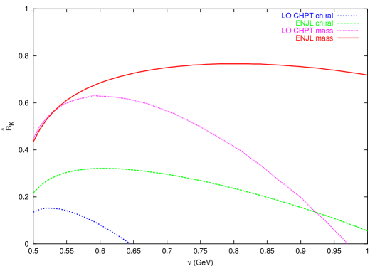
Figure 1: Matching of the short-distance scale for our $\hat{B}_{K}$ prediction. From down to up curves: using CHPT at LO in the chiral limit, using ENJL in the chiral limit, using CHPT at LO with physical masses, using ENJL with physical masses. Notice the quality of this last curve.

We got good numerical scale matching for $\hat{B}_{K}$ for the real case and not so good for the $\chi$-limit $\hat{B}_{K}^{\chi}$, see Figure 1. Our results are also analytically scheme independent [4].

$$\hat{B}_{K}^{\chi}=\frac{3}{4}(0.43\pm 0.20)=0.32\pm 0.15$$ (16)

in the chiral limit and

$$\hat{B}_{K}=0.77\pm 0.10$$ (17)

for the case of real pion and Kaon masses.

4 Results for $\varepsilon^{\prime}_{K}$

In [3] we made a prediction for $\varepsilon^{\prime}_{K}$ which we would like to update now. The new things we would like to input are the non-FSI corrections which after the work in [11, 17, 18, 19] are known. We also use the recent complete isospin breaking result of [6] and the new analytical results for $\mbox{Im}\,(e^{2}G_{E})$ [5, 12, 13]. Our result in [3] did contain the FSI corrections but not the non-FSI which were unknown at that time.

In [5, 12, 13] there are recent calculations of $\mbox{Im}\,(e^{2}G_{E})$ using dispersion relations. The results there are valid to all orders in $1/N_{c}$ and NLO in $\alpha_{S}$. They are obtained using the hadronic tau data collected by ALEPH [20] and OPAL [21] at LEP. The agreement between them is quite good and their results can be summarized in

$$\mbox{Im}\,(e^{2}G_{E})=-(4.0\pm 0.9)\,\left(\frac{87{\rm MeV}}{F_{0}}\right)^{6}\,\mbox{Im}\,\tau\,.$$ (18)

In the Standard Model

$$\mbox{Im}\,\tau=-(6.05\pm 0.50)\times 10^{-4}\,.$$ (19)

In [14], they used a Minimal Hadronic Approximation (MHA) to large $N_{c}$ QCD to calculate $\mbox{Im}\,(e^{2}G_{E})$ with the result

$$\mbox{Im}\,(e^{2}G_{E})=-(6.7\pm 2.0)\,\left(\frac{87{\rm MeV}}{F_{0}}\right)^{6}\,\mbox{Im}\,\tau\,,$$ (20)

which is also in agreement with though somewhat larger than (18). There are also lattice results for $\mbox{Im}\,(e^{2}G_{E})$ both using domain-wall fermions [22] and Wilson fermions [23]. All of them made the chiral limit extrapolations, their results are in agreement between themselves (see comparison Table in first reference in [12]) and their average gives

$$\mbox{Im}\,(e^{2}G_{E})=-(3.2\pm 0.3)\,\left(\frac{87{\rm MeV}}{F_{0}}\right)^{6}\,\mbox{Im}\,\tau\,.$$ (21)

The result we found in [3] for $\mbox{Im}\,G_{8}$ was

$$\mbox{Im}\,G_{8}=(4.4\pm 2.2)\,\left(\frac{87{\rm MeV}}{F_{0}}\right)^{4}\,\mbox{Im}\,\tau$$ (22)

at NLO in $1/N_{c}$. The uncertainty is dominated by the quark condensate error, we used [24]

$$\langle 0|\overline{q}q|0\rangle_{\overline{\rm MS}}(2{\rm GeV})=-(0.018\pm 0.004)\,{\rm GeV}^{3}$$ (23)

which agrees with the most recent sum rule determinations of this condensate and of light quark masses –see [25] for instance– and the lattice light quark masses world average [26].

We also made a calculation for $\mbox{Re}\,G_{8}$ and $G_{27}$ using the technique explained in Section 2 which reproduced the $\Delta I=1/2$ rule for Kaons within 40% through a very large $Q_{2}$ penguin-like contribution –see [2] for details. The results obtained there are

$$\mbox{Re}\,G_{8}=\left(6.0\pm 1.7\right)\,\left(\frac{87{\rm MeV}}{F_{0}}\right)^{4}\,,$$

$${\rm and}\hskip 14.22636ptG_{27}=\left(0.35\pm 0.15\right)\,\left(\frac{87{\rm MeV}}{F_{0}}\right)^{4}\,,$$ (24)

in good agreement with the results obtained in [19] from a fit of $K\to\pi\pi$ and $K\to 3\pi$ amplitudes at NLO to data

$$\mbox{Re}\,G_{8}=\left(7.0\pm 0.6\right)\,\left(\frac{87{\rm MeV}}{F_{0}}\right)^{4}\,$$

$${\rm and}\hskip 14.22636ptG_{27}=\left(0.50\pm 0.06\right)\,\left(\frac{87{\rm MeV}}{F_{0}}\right)^{4}\,.$$ (25)

Very recently, using a MHA to large $N_{c}$ QCD, the authors of [27] found qualitatively similar results to those in [2, 3]. I.e., enhancement toward the explanation of the $\Delta I=1/2$ rule trough large $Q_{2}$ penguin-like diagrams and a matrix element of the gluonic penguin $Q_{6}$ around three times the factorisable contribution. Indications of large values of $\mbox{Im}\,G_{8}$ were also found in [28].

The chiral corrections to (9), (10), and (11) can be introduced through the $C_{\Delta I=1/2}$, $C_{0}$ and $C_{2}$ factors as follows

$$\frac{\mbox{Re}\,a_{0}}{\mbox{Re}\,a_{2}} = \left(\frac{\mbox{Re}\,a_{0}}{\mbox{Re}\,a_{2}}\right)^{(2)}\,C_{\Delta I=1/2}\,;$$

$$\frac{\mbox{Im}\,a_{0}}{\mbox{Re}\,a_{0}} = \left(\frac{\mbox{Im}\,a_{0}}{\mbox{Re}\,a_{0}}\right)^{(2)}\,C_{0}\,;$$ (26)

$$\frac{\mbox{Im}\,a_{2}}{\mbox{Re}\,a_{2}} = \left(\frac{\mbox{Im}\,a_{2}}{\mbox{Re}\,a_{2}}\right)^{(2)}\,C_{2}+\Omega_{\rm eff}\,\frac{\mbox{Im}\,a_{0}}{\mbox{Re}\,a_{0}}\,.$$

The full isospin breaking corrections are included here through the effective parameter $\Omega_{\rm eff}=(0.060\pm 0.077)$ recently calculated in [6].

We get from the fit to experimental $K\to\pi\pi$ amplitudes in [19]

$$C_{\Delta I=1/2}=\frac{{\cal S}_{0}}{{\cal S}_{2}}=\frac{1.90\pm 0.16}{1.56\pm 0.19}=1.22\pm 0.15\,\,\,$$ (27)

Where ${\cal S}_{\rm I}$ are the chiral corrections to $\mbox{Re}\,a_{I}$ to all orders while we call $\cal{T}_{\rm I}$ to the chiral corrections to $\mbox{Im}\,a_{I}$ to all orders. Therefore, they contain the FSI corrections which were exhaustively studied in [17] plus the non-FSI corrections which are a sizeable effect and of opposite direction. All these chiral corrections contain the large overall known factor $f_{K}f_{\pi}^{2}/F_{0}^{3}\simeq 1.47$ from wave function renormalization.

The imaginary parts $\mbox{Im}\,a_{I}$ get FSI corrections identical to $\mbox{Re}\,a_{I}$ owing to Watson’s theorem. In addition, both due to octet dominance in $\mbox{Re}\,a_{0}$ and $\mbox{Im}\,a_{0}$ and to the numerical dominance of the non-analytic terms at NLO in $K\to\pi\pi$ amplitudes [11, 17, 19]

$$C_{0}=\,{{\cal T}_{0}}/{{\cal S}_{0}}\,\simeq 1.0\pm 0.2\,,$$ (28)

to a good approximation.

The situation is quite different for $\mbox{Im}\,a_{2}$ which is proportional to $\mbox{Im}\,(e^{2}G_{E})$ at lowest order since $\mbox{Im}\,G_{27}=0$ in the Standard Model. From the works [17, 18, 19] we also know that

$$C_{2} = \frac{{\cal T}_{2}}{{\cal S}_{2}}\simeq\frac{0.70\pm 0.21-0.73L_{4}/10^{-3}}{1.56\pm 0.18}$$ (29)

$$= 0.45\pm 0.15-0.47\frac{L_{4}}{10^{-3}}\,.$$

Putting all together, we get at LO in CHPT (using (18) and (22))

$$-\frac{1}{|\varepsilon_{K}|\sqrt{2}}\left(\frac{\mbox{Re}\,a_{2}}{\mbox{Re}\,a_{0}}\frac{\mbox{Im}\,a_{0}}{\mbox{Re}\,a_{0}}\right)^{(2)} \hskip-12.91663pt=\hskip-4.30554pt \hskip-4.30554pt-(10.8\pm 5.4)\,\mbox{Im}\,\tau\,\,$$

$$\frac{1}{|\varepsilon_{K}|\sqrt{2}}\left(\frac{\mbox{Re}\,a_{2}}{\mbox{Re}\,a_{0}}\frac{\mbox{Im}\,a_{2}}{\mbox{Re}\,a_{2}}\right)^{(2)} \hskip-12.91663pt=\hskip-4.30554pt (2.7\pm 0.8)\,\mbox{Im}\,\tau\,.$$

And therefore,

$$\left(\frac{\varepsilon^{\prime}_{K}}{\varepsilon_{K}}\right)^{(2)}=((-10.8\pm 5.4)+(2.7\pm 0.8))\,\mbox{Im}\,\tau\,$$

$$=-(8.1\pm 5.5)\,\mbox{Im}\,\tau=(4.9\pm 3.3)\times 10^{-3}\,.$$ (31)

This result is scheme independent and very stable against the short-distance scale as can be seen in Figure 2.

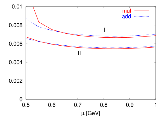
Figure 2: Matching of the short-distance scale dependence of our LO in CHPT $\varepsilon^{\prime}_{K}/\varepsilon_{K}$ prediction. Labels I and II are for two different values of $\alpha_{S}$. The two curves for two choices of perturbative matching, see [3]. Notice the quality of the matching.

The difference with the result in Figure 2 [3] is due to the new values of $\mbox{Im}\,\tau$ in (19) and $\mbox{Re}\,G_{8}$ and $G_{27}$ in (4).

Including the known and estimated higher order CHPT corrections, we get

$$-\frac{1}{|\varepsilon_{K}|\sqrt{2}}\,\frac{\mbox{Re}\,a_{2}}{\mbox{Re}\,a_{0}}\,\frac{\mbox{Im}\,a_{0}}{\mbox{Re}\,a_{0}}=-(8.9\pm 4.8)\,\mbox{Im}\,\tau\,$$ (32)

and

$$-\frac{1}{|\varepsilon_{K}|\sqrt{2}}\,\frac{\mbox{Re}\,a_{2}}{\mbox{Re}\,a_{0}}\,\frac{\mbox{Im}\,a_{2}}{\mbox{Re}\,a_{2}}=$$

$$\hskip-21.52771pt((1.0\pm 0.3)+(0.5\pm 0.7))\,\mbox{Im}\,\tau\,=(1.5\pm 0.8)\,\mbox{Im}\,\tau\,.$$

where the second part comes from isospin breaking contribution with $\Omega_{eff}=0.06\pm 0.08$ [6], and we used $L_{4}=0$ in (29). And therefore,

$$\frac{\varepsilon^{\prime}_{K}}{\varepsilon_{K}}=((-8.9\pm 4.8)+(1.5\pm 0.8))\,\mbox{Im}\,\tau\,$$

$$=-(7.4\pm 4.9)\,\mbox{Im}\,\tau=(4.5\pm 3.0)\times 10^{-3}$$ (34)

to be compared to the world average [29, 30]

$$\mbox{Re}\,\left(\frac{\varepsilon^{\prime}_{K}}{\varepsilon_{K}}\right){\Bigg{|}}_{\rm exp}=(1.66\pm 0.16)\times 10^{-3}\,.$$ (35)

Though the central value of our Standard Model prediction in (4) is a factor around 3 too large, within the big uncertainties it is still compatible with the experimental result. Two immediate consequences of the analysis above, namely, the LO CHPT prediction (4) is actually very close of the the final result (4) and second, the part with $\Delta I=1/2$ dominates when all higher order CHPT corrections are included.

5 Conclusions and Prospects

The large final uncertainty we quote in (4) is mainly due to the uncertainties of (1) the chiral limit quark condensate, which is not smaller than 20%, (2) $L_{5}$, which is around 30%, and (3) the NLO in $1/N_{c}$ corrections to the matrix element of $Q_{6}$, which is around 20%. All of them together make the present prediction for the $\Delta I=1/2$ contribution to $\varepsilon^{\prime}_{K}$ to have an error around 55%. Reduction in the uncertainty of all these inputs, especially of the quark condensate and $L_{5}$ is needed to obtain a reasonable final uncertainty.

We substituted the value used in [3] for $\mbox{Im}\,(e^{2}G_{E})$ by the one in (18), notice however that numerically they coincide within errors. There are also large uncertainties in the $\Delta I=3/2$ component coming from isospin breaking [6], and more moderate in the non-FSI corrections to $\mbox{Im}\,a_{2}$, fortunately the impact of them in the final result is not as large as the ones associated to the $\Delta I=1/2$ component.

Assuming the $\Delta I=3/2$ component of $\varepsilon^{\prime}_{K}$ is fixed to be the one in (18) as indicated by the analytic methods [5, 12, 13, 14] and lattice [22, 23], one can try to extract the value of $\mbox{Im}\,G_{8}$ from the experimental result in (35). We get

$$\mbox{Im}\,G_{8}=(2.0^{+0.7}_{-0.4})\,\left(\frac{87{\rm MeV}}{F_{0}}\right)^{4}\,\mbox{Im}\,\tau$$ (36)

i.e. the central value coincides with the large $N_{c}$ result for $\mbox{Im}\,G_{8}$ within 30% of uncertainty. This value has to be compared to our result in (22).

We have presented in [31] a ladder resummation hadronic model which keeps the good features of the ENJL model –CHPT at NLO, for instance– and improves adding more short-distance QCD constraints and the analytic structure of large $N_{c}$. We intend to use the Green’s functions calculated within this hadronic model analytically, and study the relevant internal cancellations and dominant hadronic parameters in the quantities we calculate with them. Work in this direction where we will study the origin of the large chiral corrections to $\hat{B}_{K}$ we found in [1] is in progress [32]. This program will also be extended to study the origin of the large value for $\mbox{Im}\,G_{8}$ in (22) which we got in [3]. Large values of $\mbox{Im}\,G_{8}$ were previously pointed out in [28] and more recently in [27].

References

- [1] J. Bijnens and J. Prades, Phys. Lett. B 342 (1995) 331 [arXiv:hep-ph/9409255]; Nucl. Phys. B 444 (1995) 523 [arXiv:hep-ph/9502363].
- [2] J. Bijnens and J. Prades, J. High Energy Phys. 01 (1999) 023 [arXiv:hep-ph/9811472]; J. Prades, Nucl. Phys. B (Proc. Suppl.) 86 (2000) 294 [arXiv:hep-ph/9909245]; J. Bijnens, arXiv:hep-ph/9907514.
- [3] J. Bijnens and J. Prades, J. High Energy Phys. 06 (2000) 035 [arXiv:hep-ph/0005189]; arXiv:hep-ph/0009155; arXiv:hep-ph/0009156; Nucl. Phys. B (Proc. Suppl.) 96 (2001) 354 [arXiv:hep-ph/0010008].
- [4] J. Bijnens and J. Prades, J. High Energy Phys. 01 (2000) 002 [arXiv:hep-ph/9911392].
- [5] J. Bijnens, E. Gámiz and J. Prades, J. High Energy Phys. 10 (2001) 009 [arXiv:hep-ph/0108240]; arXiv:hep-ph/0209089.
- [6] V. Cirigliano, A. Pich, G. Ecker and H. Neufeld, arXiv:hep-ph/0307030.
- [7] J. Bijnens, E. Pallante and J. Prades, Nucl. Phys. B 626 (2002) 410 [arXiv:hep-ph/0112255]; Nucl. Phys. B 474 (1996) 379 [arXiv:hep-ph/9511388]; Phys. Rev. Lett. 75 (1995) 1447 [Erratum-ibid. 75 (1995) 3781] [arXiv:hep-ph/9505251]; J. Prades, arXiv:hep-ph/0108192.
- [8] J. Bijnens and J. Prades, Nucl. Phys. B 490 (1997) 239 [arXiv:hep-ph/9610360].
- [9] M. Battaglia et al., arXiv:hep-ph/0304132; M. Ciuchini, E. Franco, F. Parodi, V. Lubicz, L. Silvestrini and A. Stocchi, arXiv:hep-ph/0307195.
- [10] G. Ecker, arXiv:hep-ph/0011026; A. Pich, arXiv:hep-ph/9806303.
- [11] J. Bijnens, E. Pallante and J. Prades, Nucl. Phys. B 521 (1998) 305 [arXiv:hep-ph/9801326].
- [12] V. Cirigliano, J.F. Donoghue, E. Golowich and K. Maltman, Phys. Lett. B 555 (2003) 71 [arXiv:hep-ph/0211420]; Phys. Lett. B 522 (2001) 245 [arXiv:hep-ph/0109113]; J.F. Donoghue and E. Golowich, Phys. Lett. B 478 (2000) 172 [arXiv:hep-ph/9911309].
- [13] S. Narison, Nucl. Phys. B 593 (2001) 3 [arXiv:hep-ph/0004247].
- [14] M. Knecht, S. Peris and E. de Rafael, Phys. Lett. B 508 (2001) 117 [arXiv:hep-ph/0102017]; Phys. Lett. B 457 (1999) 227 [arXiv:hep-ph/9812471].
- [15] J. Bijnens, C. Bruno and E. de Rafael, Nucl. Phys. B 390 (1993) 501 [arXiv:hep-ph/9206236]; J. Prades, Z. Phys. C 63 (1994) 491 [Erratum Eur. J. Phys. C 11 (1999) 571] [arXiv:hep-ph/9302246]; J. Bijnens, E. de Rafael and H.q. Zheng, Z. Phys. C 62 (1994) 437 [arXiv:hep-ph/9306323]; J. Bijnens and J. Prades, Phys. Lett. B 320 (1994) 130 [arXiv:hep-ph/9310355]; Z. Phys. C 64 (1994) 475 [arXiv:hep-ph/9403233].; Nucl. Phys. B (Proc. Suppl.) 39BC (1995) 245 [arXiv:hep-ph/9409231]; J. Bijnens, Phys. Rept. 265 (1996) 369 [arXiv:hep-ph/9502335].
- [16] S. Peris, M. Perrottet and E. de Rafael, J. High Energy Phys. 05 (1998) 011 [arXiv:hep-ph/9805442].
- [17] E. Pallante, A. Pich and I. Scimemi, Nucl. Phys. B 617 (2001) 441 [arXiv:hep-ph/0105011]; E. Pallante and A. Pich, Nucl. Phys. B 592 (2001) 294 [arXiv:hep-ph/0007208]; Phys. Rev. Lett. 84 (2000) 2568 [arXiv:hep-ph/9911233].
- [18] V. Cirigliano and E. Golowich, Phys. Rev. D 65 (2002) 054014 [arXiv:hep-ph/0109265]; Phys. Lett. B 475 (2000) 351 [arXiv:hep-ph/9912513].
- [19] J. Bijnens, P. Dhonte and F. Persson, Nucl. Phys. B 648 (2003) 317 [arXiv:hep-ph/0205341].
- [20] R. Barate et al. [ALEPH Collaboration], Eur. Phys. J. C 4 (1998) 409.
- [21] K. Ackerstaff et al. [OPAL Collaboration], Eur. Phys. J. C 7 (1999) 571 [arXiv:hep-ex/9808019].
- [22] J.I. Noaki et al. [CP-PACS Collaboration], Phys. Rev. D 68 (2003) 014501 [arXiv:hep-lat/0108013]; T. Blum et al. [RBC Collaboration], arXiv:hep-lat/0110075.
- [23] D. Bećirević et al. [SPQCDR Collaboration], arXiv:hep-lat/0209136.
- [24] J. Bijnens, J. Prades and E. de Rafael, Phys. Lett. B 348 (1995) 226 [arXiv:hep-ph/9411285]; J. Prades, Nucl. Phys. B (Proc. Suppl.) 64 (1998) 253 [arXiv:hep-ph/9708395].
- [25] M. Jamin, Phys. Lett. B 538 (2002) 71 [arXiv:hep-ph/0201174]; M. Jamin, J.A. Oller and A. Pich, Eur. Phys. J. C 24 (2002) 237 [arXiv:hep-ph/0110194]; K. Maltman and J. Kambor, Phys. Lett. B 517 (2001) 332 [arXiv:hep-ph/0107060].
- [26] H. Wittig, arXiv:hep-lat/0210025.
- [27] T. Hambye, S. Peris and E. de Rafael, J. High Energy Phys. 05 (2003) 027 [arXiv:hep-ph/0305104].
- [28] T. Hambye, G.O. Köhler, E.A. Paschos and P.H. Soldan, Nucl. Phys. B 564 (2000) 391 [arXiv:hep-ph/9906434]; T. Hambye, G.O. Köhler, E.A. Paschos, P.H. Soldan and W.A. Bardeen, Phys. Rev. D 58 (1998) 014017 [arXiv:hep-ph/9802300].
- [29] J.R. Batley et al. [NA48 Collaboration], Phys. Lett. B 544 (2002) 97 [arXiv:hep-ex/0208009].
- [30] A. Alavi-Harati et al. [KTeV Collaboration], Phys. Rev. D 67 (2003) 012005 [arXiv:hep-ex/0208007].
- [31] J. Bijnens, E. Gámiz, E. Lipartia and J. Prades, J. High Energy Phys. 04 (2003) 055 [arXiv:hep-ph/0304222].
- [32] J. Bijnens, E. Gámiz, E. Lipartia and J. Prades, work in preparation.