Quantum Field Theory of particle mixing and oscillations

Abstract

We report on recent results on the Quantum Field Theory of mixed particles. The quantization procedure is discussed in detail, both for fermions and for bosons and the unitary inequivalence of the flavor and mass representations is proved. Oscillation formulas exhibiting corrections with respect to the usual quantum mechanical ones are then derived.

1 Introduction

The chapter of particle mixing and oscillations [1] is one of the most important and fascinating in the book of modern Particle Physics. This is especially true after the recent experimental results [2] which finally confirm, after a long search, the reality of neutrino oscillations [3, 4]: this represents indeed the first clear evidence for physics beyond the Standard Model.

Many unanswered questions about the physics of particle mixing are however still there, in particular from a theoretical point of view. Apart from the problem of the origin of mixing and of the small neutrino masses, difficulties arise already in the attempt to find a proper mathematical setting for the description of mixed particles in Quantum Field Theory (QFT).

It is indeed well known [5] that mixing of states with different masses is not allowed in non-relativistic Quantum Mechanics (QM). In spite of this fact, the quantum mechanical treatment is the one usually adopted for its simplicity and elegance. A review of the problems connected with the QM of mixing and oscillations can be found in Ref.[7]. Difficulties in the construction of the Hilbert space for mixed neutrinos were pointed out in Ref.[8].

Only recently [9]-[22] a consistent treatment of mixing and oscillations in QFT has been achieved and we report here on these results.

The main point of our analysis [9] consists in the observation that a problem of representation (i.e. choice of the Hilbert space) may arise when we start to mix fields with different masses. This has to do with the peculiar mathematical structure of QFT, where unitarily inequivalent representations of the algebra of fields do exist [23, 24]: a classical example is the one of theories with spontaneous breakdown of symmetry. This situation is in contrast to the one of QM, which deals with systems with a finite number of degrees of freedom and where only one Hilbert space is admitted (von Neumann theorem).

On this basis, a careful analysis of the usual mixing transformations in QFT reveals a rich non-perturbative structure associated to the vacuum for mixed particles, which appears to be a condensate of particle-antiparticle pairs, both for fermions and bosons. The vacuum for the mixed fields is a generalized coherent state à la Perelomov [25].

The structure of flavor vacuum reflects into observable quantities: exact oscillation formulas [11, 18] are derived in QFT exhibiting corrections with respect to the usual QM ones. We also show that a geometric phase is associated to flavor oscillations [26].

The material here presented is organized in the following way:

In Section 2, the mixing transformations are studied in QFT, both for fermions and bosons, in the case of two flavors. The currents and charges for mixed fields are also introduced and then used in Section 3 to derive exact oscillation formulas for charged fields (bosons and fermions). The case of neutral fields is treated in Section 3.3.

The geometric phase for oscillating particles is studied in Section 4. In Section 5 the case of three flavor mixing is considered and the deformation of the associated algebra due to CP violation is discussed. Finally, in Section 6, a space dependent oscillation formula for neutrinos is derived using the relativistic flavor current.

2 Mixing transformations in Quantum Field Theory

In this Section we study the quantization of mixed fields both for Dirac fermions and for charged bosons [9, 10, 18]. For simplicity, we limit ourselves to the case of two generations (flavors) although the main results presented below have general validity [14]. Three flavor fermion mixing [19] is discussed in §5.

2.1 Fermion mixing

Let us consider two flavor fields $\nu_{e}$, $\nu_{\mu}$. The mixing relations are [3]

$$\nu_{e}(x) = \cos\theta\;\nu_{1}(x)\,+\,\sin\theta\;\nu_{2}(x)$$

$$\nu_{\mu}(x) = -\sin\theta\;\nu_{1}(x)\,+\,\cos\theta\;\nu_{2}(x)\;,$$ (1)

Here $\nu_{e}$, $\nu_{\mu}$ are the (Dirac) neutrino fields with definite flavors. $\nu_{1}$, $\nu_{2}$ are the (free) neutrino fields with definite masses $m_{1}$, $m_{2}$, respectively. $\theta$ is the mixing angle. The fields $\nu_{1}$ and $\nu_{2}$ are expanded as

$$\nu_{i}(x)=\frac{1}{\sqrt{V}}\sum_{{\bf k},r}\left[u^{r}_{{\bf k},i}(t)\alpha^{r}_{{\bf k},i}\>+v^{r}_{-{\bf k},i}(t)\beta^{r{\dagger}}_{-{\bf k},i}\right]e^{i{\bf k}\cdot{\bf x}},\;\quad i=1,2\;.$$ (2)

where $u^{r}_{{\bf k},i}(t)=e^{-i\omega_{k,i}t}u^{r}_{{\bf k},i}$ and $v^{r}_{{\bf k},i}(t)=e^{i\omega_{k,i}t}v^{r}_{{\bf k},i}$, with $\omega_{k,i}=\sqrt{{\bf k}^{2}+m_{i}^{2}}$. The $\alpha^{r}_{{\bf k},i}$ and the $\beta^{r}_{{\bf k},i}$ ($r=1,2$), are the annihilation operators for the vacuum state $|0\rangle_{1,2}\equiv|0\rangle_{1}\otimes|0\rangle_{2}$: $\alpha^{r}_{{\bf k},i}|0\rangle_{1,2}=\beta^{r}_{{\bf k},i}|0\rangle_{1,2}=0$. The anticommutation relations are:

$$\{\nu^{\alpha}_{i}(x),\nu^{\beta{\dagger}}_{j}(y)\}_{t=t^{\prime}}=\delta^{3}({\bf x}-{\bf y})\delta_{\alpha\beta}\delta_{ij}\;,\;\;\;\;\;\alpha,\beta=1,..,4\;,$$ (3)

$$\{\alpha^{r}_{{\bf k},i},\alpha^{s{\dagger}}_{{\bf q},j}\}=\delta_{{\bf k}q}\delta_{rs}\delta_{ij};\qquad\{\beta^{r}_{{\bf k},i},\beta^{s{\dagger}}_{{\bf q},j}\}=\delta_{{\bf k}q}\delta_{rs}\delta_{ij},\;\;\;\;i,j=1,2\;.$$ (4)

All other anticommutators are zero. The orthonormality and completeness relations are:

$$u^{r{\dagger}}_{{\bf k},i}u^{s}_{{\bf k},i}=v^{r{\dagger}}_{{\bf k},i}v^{s}_{{\bf k},i}=\delta_{rs}\;,\quad u^{r{\dagger}}_{{\bf k},i}v^{s}_{-{\bf k},i}=v^{r{\dagger}}_{-{\bf k},i}u^{s}_{{\bf k},i}=0\;,$$ (5)

$$\sum_{r}(u^{r}_{{\bf k},i}u^{r{\dagger}}_{{\bf k},i}+v^{r}_{-{\bf k},i}v^{r{\dagger}}_{-{\bf k},i})=1{\rm I}\;.$$ (6)

In QFT the basic dynamics, i.e. the Lagrangian and the resulting field equations, is given in terms of Heisenberg (or interacting) fields. The physical observables are expressed in terms of asymptotic in- (or out-) fields, also called physical or free fields. In the LSZ formalism of QFT [23, 24], the free fields, say for definitiveness the in-fields, are obtained by the weak limit of the Heisenberg fields for time $t\rightarrow-\infty$. The meaning of the weak limit is that the realization of the basic dynamics in terms of the in-fields is not unique so that the limit for $t\rightarrow-\infty$ (or $t\rightarrow+\infty$ for the out-fields) is representation dependent.

Typical examples are the ones of spontaneously broken symmetry theories, where the same set of Heisenberg field equations describes the normal (symmetric) phase as well as the symmetry broken phase. Since observables are described in terms of asymptotic fields, unitarily inequivalent representations describe different, i.e. physically inequivalent, phases. It is therefore of crucial importance, in order to get physically meaningful results, to investigate with much care the mapping among Heisenberg or interacting fields and free fields, i.e. the dynamical map.

With this warnings, mixing relations such as the relations (1) deserve a careful analysis, since they actually represent a dynamical mapping. It is now our purpose to investigate the structure of the Fock spaces ${\cal H}_{1,2}$ and ${\cal H}_{e,\mu}$ relative to $\nu_{1}$, $\nu_{2}$ and $\nu_{e}$, $\nu_{\mu}$, respectively. In particular we want to study the relation among these spaces in the infinite volume limit. As usual, we will perform all computations at finite volume $V$ and only at the end we will put $V\rightarrow\infty$.

Our first step is the study of the generator of Eqs.(1) and of the underlying group theoretical structure. Eqs.(1) can be recast as [9]:

$$\nu_{e}^{\alpha}(x) = G^{-1}_{\theta}(t)\;\nu_{1}^{\alpha}(x)\;G_{\theta}(t)$$ (7)

$$\nu_{\mu}^{\alpha}(x) = G^{-1}_{\theta}(t)\;\nu_{2}^{\alpha}(x)\;G_{\theta}(t)\;,$$ (8)

where $G_{\theta}(t)$ is given by

$$G_{\theta}(t)=\exp\left[\theta\int d^{3}{\bf x}\left(\nu_{1}^{{\dagger}}(x)\nu_{2}(x)-\nu_{2}^{{\dagger}}(x)\nu_{1}(x)\right)\right]\;,$$ (9)

and is (at finite volume) an unitary operator: $G^{-1}_{\theta}(t)=G_{-\theta}(t)=G^{{\dagger}}_{\theta}(t)$, preserving the canonical anticommutation relations (3). Eq.(9) follows from $\frac{d^{2}}{d\theta^{2}}\nu^{\alpha}_{e}=-\nu^{\alpha}_{e}\;,\;\;\;\frac{d^{2}}{d\theta^{2}}\nu^{\alpha}_{\mu}=-\nu^{\alpha}_{\mu}$ with the initial conditions $\nu^{\alpha}_{e}|_{\theta=0}=\nu^{\alpha}_{1}$, $\frac{d}{d\theta}\nu^{\alpha}_{e}|_{\theta=0}=\nu^{\alpha}_{2}$ and $\nu^{\alpha}_{\mu}|_{\theta=0}=\nu^{\alpha}_{2}$, $\frac{d}{d\theta}\nu^{\alpha}_{\mu}|_{\theta=0}=-\nu^{\alpha}_{1}$.

Note that $G_{\theta}$ is an element of $SU(2)$ since it can be written as

$$G_{\theta}(t)=\exp[\theta(S_{+}(t)-S_{-}(t))]\;,$$ (10)

$$S_{+}(t)=S^{{\dagger}}_{-}(t)\equiv\int d^{3}{\bf x}\;\nu_{1}^{{\dagger}}(x)\nu_{2}(x)\,.$$ (11)

By introducing then

$$S_{3}\equiv\frac{1}{2}\int d^{3}{\bf x}\left(\nu_{1}^{{\dagger}}(x)\nu_{1}(x)-\nu_{2}^{{\dagger}}(x)\nu_{2}(x)\right)\;,$$ (12)

the $su(2)$ algebra is closed (for $t$ fixed):

$$[S_{+}(t),S_{-}(t)]=2S_{3}\;\;\;,\;\;\;[S_{3},S_{\pm}(t)]=\pm S_{\pm}(t)\;.$$ (13)

The action of the mixing generator on the vacuum $|0\rangle_{1,2}$ is non-trivial and we have (at finite volume $V$):

$$|0(t)\rangle_{e,\mu}\equiv G^{-1}_{\theta}(t)\;|0\rangle_{1,2}\;.$$ (14)

$|0(t)\rangle_{e,\mu}$ is the flavor vacuum, i.e. the vacuum for the flavor fields. Note that $G^{-1}_{\theta}(t)$ is just the generator for generalized coherent states of $SU(2)$ [25]: the flavor vacuum is therefore an $SU(2)$ (time dependent) coherent state. Let us now investigate the infinite volume limit of Eq.(14). Using the Gaussian decomposition, $G^{-1}_{\theta}$ is written as [25]

$$\exp[\theta(S_{-}-S_{+})]=\exp(-\tan\theta\;S_{+})\;\exp(-2\ln\>\cos\theta\;S_{3})\;\exp(\tan\theta\;S_{-})$$

where $0\leq\theta<\frac{\pi}{2}$. We then compute ${}_{1,2}\langle 0|0(t)\rangle_{e,\mu}$ and obtain

$${}_{1,2}\langle 0|0(t)\rangle_{e,\mu}=\prod_{{\bf k}}\left(1-\sin^{2}\theta\;|V_{{\bf k}}|^{2}\right)^{2}\equiv\prod_{{\bf k}}\Gamma(k)=e^{\sum_{{\bf k}}ln\;\Gamma(k)}.$$ (15)

where the function $|V_{{\bf k}}|^{2}$ is defined in Eq.(25) and plotted in Fig.1. Note that $|V_{\bf k}|^{2}$ depends on ${|\bf k}|$, it is always in the interval $[0,\frac{1}{2}[$ and goes to zero for $|{\bf k}|\rightarrow\infty$. By using the customary continuous limit relation $\sum_{{\bf k}}\;\rightarrow\;\frac{V}{(2\pi)^{3}}\int d^{3}{\bf k}$, in the infinite volume limit we obtain (for any $t$)

$$\lim_{V\rightarrow\infty}\;{}_{1,2}\langle 0|0(t)\rangle_{e,\mu}=\lim_{V\rightarrow\infty}\;e^{\frac{V}{(2\pi)^{3}}\int d^{3}{\bf k}\;ln\;\Gamma(k)}=0$$ (16)

since $\Gamma({\bf k})<1$ for any value of ${\bf k}$ and of $m_{1}$ and $m_{2}$ (with $m_{2}\neq m_{1}$).

Notice that (16) shows that the orthogonality between $|0(t)\rangle_{e,\mu}$ and $|0\rangle_{1,2}$ is due to the infrared contributions which are taken in care by the infinite volume limit and therefore high momentum contributions do not influence the result (for this reason here we do not need to consider the regularization problem of the UV divergence of the integral of $\ln\;\Gamma({\bf k})$). Of course, this orthogonality disappears when $\theta=0$ and/or when $m_{1}=m_{2}$ (in this case $V_{{\bf k}}=0$ for any ${\bf k}$ ).

Eq.(16) expresses the unitary inequivalence in the infinite volume limit of the flavor and the mass representations and shows the non-trivial nature of the mixing transformations (1), resulting in the condensate structure of the flavor vacuum. In Section 3 we will see how such a vacuum structure leads to phenomenological consequences in the neutrino oscillations, which may be possibly experimentally tested.

By use of $G_{\theta}(t)$, the flavor fields can be expanded as:

$${}\nu_{\sigma}(x)\,=\,\sum_{r=1,2}\int\frac{d^{3}{\bf{k}}}{(2\pi)^{\frac{3}{2}}}\left[u^{r}_{{\bf k},i}(t)\alpha^{r}_{{\bf k},\sigma}(t)+v^{r}_{-{\bf k},i}(t)\beta^{r{\dagger}}_{-{\bf k},\sigma}(t)\right]e^{i{\bf k}\cdot{\bf x}}\,,$$ (17)

with $(\sigma,i)=(e,1),(\mu,2)$. The flavor annihilation operators are defined as $\alpha^{r}_{{\bf k},\sigma}(t)\equiv G^{-1}_{\bf\theta}(t)\alpha^{r}_{{\bf k},i}G_{\bf\theta}(t)$ and $\beta^{r{\dagger}}_{{-\bf k},\sigma}(t)\equiv G^{-1}_{\bf\theta}(t)\beta^{r{\dagger}}_{{-\bf k},i}G_{\bf\theta}(t)$. In the reference frame such that ${\bf k}=(0,0,|{\bf k}|)$, we have the simple expressions:

$${}\alpha^{r}_{{\bf k},e}(t)=\cos\theta\;\alpha^{r}_{{\bf k},1}\;+\;\sin\theta\;\left(U_{{\bf k}}^{*}(t)\;\alpha^{r}_{{\bf k},2}\;+\;\epsilon^{r}\;V_{{\bf k}}(t)\;\beta^{r{\dagger}}_{-{\bf k},2}\right)$$ (18)

$${}\alpha^{r}_{{\bf k},\mu}(t)=\cos\theta\;\alpha^{r}_{{\bf k},2}\;-\;\sin\theta\;\left(U_{{\bf k}}(t)\;\alpha^{r}_{{\bf k},1}\;-\;\epsilon^{r}\;V_{{\bf k}}(t)\;\beta^{r{\dagger}}_{-{\bf k},1}\right)$$ (19)

$${}\beta^{r}_{-{\bf k},e}(t)=\cos\theta\;\beta^{r}_{-{\bf k},1}\;+\;\sin\theta\;\left(U_{{\bf k}}^{*}(t)\;\beta^{r}_{-{\bf k},2}\;-\;\epsilon^{r}\;V_{{\bf k}}(t)\;\alpha^{r{\dagger}}_{{\bf k},2}\right)$$ (20)

$${}\beta^{r}_{-{\bf k},\mu}(t)=\cos\theta\;\beta^{r}_{-{\bf k},2}\;-\;\sin\theta\;\left(U_{{\bf k}}(t)\;\beta^{r}_{-{\bf k},1}\;+\;\epsilon^{r}\;V_{{\bf k}}(t)\;\alpha^{r{\dagger}}_{{\bf k},1}\right)$$ (21)

where $\epsilon^{r}=(-1)^{r}$ and

$${}U_{{\bf k}}(t)\equiv u^{r{\dagger}}_{{\bf k},2}(t)u^{r}_{{\bf k},1}(t)=v^{r{\dagger}}_{-{\bf k},1}(t)v^{r}_{-{\bf k},2}(t)=\,|U_{{\bf k}}|\,e^{i(\omega_{k,2}-\omega_{k,1})t}$$ (22)

$${}V_{{\bf k}}(t)\equiv\epsilon^{r}\;u^{r{\dagger}}_{{\bf k},1}(t)v^{r}_{-{\bf k},2}(t)=-\epsilon^{r}\;u^{r{\dagger}}_{{\bf k},2}(t)v^{r}_{-{\bf k},1}(t)=\,|V_{{\bf k}}|\;e^{i(\omega_{k,2}+\omega_{k,1})t}$$ (23)

$$|U_{{\bf k}}|=\frac{|{\bf k}|^{2}+(\omega_{k,1}+m_{1})(\omega_{k,2}+m_{2})}{2\sqrt{\omega_{k,1}\omega_{k,2}(\omega_{k,1}+m_{1})(\omega_{k,2}+m_{2})}}$$ (24)

$$|V_{{\bf k}}|=\frac{(\omega_{k,1}+m_{1})-(\omega_{k,2}+m_{2})}{2\sqrt{\omega_{k,1}\omega_{k,2}(\omega_{k,1}+m_{1})(\omega_{k,2}+m_{2})}}\,|{\bf k}|$$ (25)

$$|U_{{\bf k}}|^{2}+|V_{{\bf k}}|^{2}=1.$$ (26)

Figure 1: The fermion condensation density $|V_{\bf k}|^{2}$ as a function of $|{\bf k}|$ for $m_{1}=1$, $m_{2}=100$ (solid line) and $m_{1}=10$, $m_{2}=100$ (dashed line).

The condensation density of the flavor vacuum is given by

$$\;{}_{e,\mu}\langle 0(t)|\alpha_{{\bf k},i}^{r{\dagger}}\alpha^{r}_{{\bf k},i}|0(t)\rangle_{e,\mu}=\sin^{2}\theta\;|V_{{\bf k}}|^{2},\qquad i=1,2\,,$$ (27)

with the same result for antiparticles. Note that the $|V_{{\bf k}}|^{2}$ has a maximum at $\sqrt{m_{1}m_{2}}$ and $|V_{{\bf k}}|^{2}\simeq\frac{(m_{{}_{2}}-m_{{}_{1}})^{2}}{4|{\bf k}|^{2}}$ for $|{\bf k}|\gg\sqrt{m_{{}_{1}}m_{{}_{2}}}$.

2.2 Boson mixing

Let us now consider boson mixing [10, 18] in the case of charged fields. We define the mixing relations as:

$$\phi_{A}(x) = \cos\theta\;\phi_{1}(x)+\sin\theta\;\phi_{2}(x)$$

$$\phi_{B}(x) = -\sin\theta\;\phi_{1}(x)+\cos\theta\;\phi_{2}(x)$$ (28)

where generically we denote the mixed fields with suffixes $A$ and $B$. Let the fields $\phi_{i}(x)$, $i=1,2$, be free complex fields with definite masses. Their conjugate momenta are $\pi_{i}(x)=\partial_{0}\phi_{i}^{{\dagger}}(x)$ and the commutation relations are the usual ones:

$$\left[\phi_{i}(x),\pi_{j}(y)\right]_{t=t^{\prime}}=\left[\phi_{i}^{{\dagger}}(x),\pi_{j}^{{\dagger}}(y)\right]_{t=t^{\prime}}=i\delta^{3}({\bf x}-{\bf y})\,\delta_{ij}$$ (29)

with $i,j=1,2$ and the other equal–time commutators vanishing. The Fourier expansions of fields and momenta are:

$$\phi_{i}(x)=\int\frac{d^{3}{\bf k}}{(2\pi)^{\frac{3}{2}}}\frac{1}{\sqrt{2\omega_{k,i}}}\left(a_{{\bf k},i}\,e^{-i\omega_{k,i}t}+b^{{\dagger}}_{-{\bf k},i}\,e^{i\omega_{k,i}t}\right)e^{i{\bf k}\cdot{\bf x}}$$ (30)

$$\pi_{i}(x)=i\,\int\frac{d^{3}{\bf k}}{(2\pi)^{\frac{3}{2}}}\sqrt{\frac{\omega_{k,i}}{2}}\left(a^{{\dagger}}_{{\bf k},i}\,e^{i\omega_{k,i}t}-b_{-{\bf k},i}\,e^{-i\omega_{k,i}t}\right)e^{i{\bf k}\cdot{\bf x}}\,,$$ (31)

where $\omega_{k,i}=\sqrt{{\bf k}^{2}+m_{i}^{2}}$ and $\left[a_{{\bf k},i},a_{{\bf p},j}^{{\dagger}}\right]=\left[b_{{\bf k},i},b_{{\bf p},j}^{{\dagger}}\right]=\delta^{3}({\bf k}-{\bf p})\delta_{ij}\,,$ with $i,j=1,2\,$ and the other commutators vanishing.

We proceed in a similar way as for fermions and write Eqs.(28) as

$$\phi_{\sigma}(x) = G^{-1}_{\theta}(t)\;\phi_{i}(x)\;G_{\theta}(t)$$ (32)

with $(\sigma,i)=(A,1),(B,2)$, and similar expressions for $\pi_{A}$, $\pi_{B}$. We have

$$G_{\theta}(t)=\exp[\theta(S_{+}(t)-S_{-}(t))]~{}.$$ (33)

The operators

$$S_{+}(t)=S_{-}^{{\dagger}}(t)\equiv-i\;\int d^{3}{\bf x}\;(\pi_{1}(x)\phi_{2}(x)-\phi_{1}^{{\dagger}}(x)\pi_{2}^{{\dagger}}(x))\,,$$

$${}S_{3}\equiv\frac{-i}{2}\int d^{3}{\bf x}\left(\pi_{1}(x)\phi_{1}(x)-\phi_{1}^{{\dagger}}(x)\pi_{1}^{{\dagger}}(x)-\pi_{2}(x)\phi_{2}(x)+\phi_{2}^{{\dagger}}(x)\pi_{2}^{{\dagger}}(x)\right)$$

close the $su(2)$ algebra (at a given $t$).

As for fermions, the action of the generator of the mixing transformations on the vacuum $|0\rangle_{1,2}$ for the fields $\phi_{1,2}$ is non-trivial and induces on it a $SU(2)$ coherent state structure [25]:

$$|0(t)\rangle_{{}_{A,B}}\equiv G^{-1}_{\theta}(t)\;|0\rangle_{1,2}\,.$$ (36)

We will refer to the state $|0(t)\rangle_{{}_{A,B}}$ as to the flavor vacuum for bosons. The orthogonality between $|0(t)\rangle_{{}_{A,B}}$ and $|0\rangle_{1,2}$ can be proved [18]. The Fourier expansion for the flavor fields is:

$$\phi_{\sigma}(x)=\int\frac{d^{3}{\bf k}}{(2\pi)^{\frac{3}{2}}}\frac{1}{\sqrt{2\omega_{k,i}}}\left(a_{{\bf k},\sigma}(t)\,e^{-i\omega_{k,i}t}+b^{{\dagger}}_{-{\bf k},\sigma}(t)\,e^{i\omega_{k,i}t}\right)e^{i{\bf k}\cdot{\bf x}}$$ (37)

with $(\sigma,i)=(A,1),(B,2)$, and similar expressions for $\pi_{A}$, $\pi_{B}$.

The annihilation operators for the vacuum $|0(t)\rangle_{{}_{A,B}}$ are defined $a_{{\bf k},A}(t)\equiv G^{-1}_{\theta}(t)\;a_{{\bf k},1}\;G_{\theta}(t)$, etc. We have:

$${}a_{{\bf k},A}(t)\,=\,\cos\theta\;a_{{\bf k},1}\;+\;\sin\theta\;\left(U^{*}_{{\bf k}}(t)\;a_{{\bf k},2}\;+\;V_{{\bf k}}(t)\;b^{{\dagger}}_{-{\bf k},2}\right)\,,$$ (38)

$${}a_{{\bf k},B}(t)\,=\,\cos\theta\;a_{{\bf k},2}\;-\;\sin\theta\;\left(U_{{\bf k}}(t)\;a_{{\bf k},1}\;-\;V_{{\bf k}}(t)\;b^{{\dagger}}_{-{\bf k},1}\right)\,,$$ (39)

$${}b_{-{\bf k},A}(t)\,=\,\cos\theta\;b_{-{\bf k},1}\;+\;\sin\theta\;\left(U^{*}_{{\bf k}}(t)\;b_{-{\bf k},2}\;+\;V_{{\bf k}}(t)\;a^{{\dagger}}_{{\bf k},2}\right)\,,$$ (40)

$${}b_{-{\bf k},B}(t)\,=\,\cos\theta\;b_{-{\bf k},2}\;-\;\sin\theta\;\left(U_{{\bf k}}(t)\;b_{-{\bf k},1}\;-\;V_{{\bf k}}(t)\;a^{{\dagger}}_{{\bf k},1}\right)~{}.$$ (41)

These operators satisfy the canonical commutation relations (at equal times).

Figure 2: The boson condensation density $|V_{\bf k}|^{2}$ as a function of $|{\bf k}|$ for $m_{1}=1$, $m_{2}=10$ (solid line) and $m_{1}=2$, $m_{2}=10$ (dashed line).

As for the case of the fermion mixing, the structure of the flavor ladder operators Eqs.(38)-(41) is recognized to be the one of a rotation combined with a Bogoliubov transformation. Indeed, in the above equations appear the Bogoliubov coefficients:

$${}U_{{\bf k}}(t)\equiv|U_{{\bf k}}|\;e^{i(\omega_{k,2}-\omega_{k,1})t}\quad,\quad V_{{\bf k}}(t)\equiv|V_{{\bf k}}|\;e^{i(\omega_{k,1}+\omega_{k,2})t}$$ (42)

$${}|U_{{\bf k}}|\equiv\frac{1}{2}\left(\sqrt{\frac{\omega_{k,1}}{\omega_{k,2}}}+\sqrt{\frac{\omega_{k,2}}{\omega_{k,1}}}\right)\;,\quad|V_{{\bf k}}|\equiv\frac{1}{2}\left(\sqrt{\frac{\omega_{k,1}}{\omega_{k,2}}}-\sqrt{\frac{\omega_{k,2}}{\omega_{k,1}}}\right)$$ (43)

$${}|U_{{\bf k}}|^{2}-|V_{{\bf k}}|^{2}=1\,,$$ (44)

Note the difference with respect to the fermionic case Eq.(26).

The condensation density of the flavor vacuum is given for any $t$ by

$${}_{{}_{A,B}}\langle 0(t)|a_{{\bf k},i}^{{\dagger}}a_{{\bf k},i}|0(t)\rangle_{{}_{A,B}}=\,\sin^{2}\theta\;|V_{{\bf k}}|^{2},\qquad i=1,2\,,$$ (45)

with same result for antiparticles. The function $|V_{{\bf k}}|^{2}$ is maximal at $|{\bf k}|=0$ ($|V_{max}|^{2}=\frac{(m_{1}-m_{2})^{2}}{4m_{1}m_{2}}$) and $|V_{{\bf k}}|^{2}\simeq\left(\frac{\Delta m^{2}}{4|{\bf k}|^{2}}\right)^{2}$ for $|{\bf k}|^{2}\gg\frac{m_{{}_{1}}^{2}+m_{{}_{2}}^{2}}{2}$. A plot is given in Fig.2 for sample values of the masses.

2.3 Currents and charges for mixed fields

We now study the transformations acting on a doublet of free fields with different masses. The results of this Section clarify the meaning of the $su(2)$ algebraic structure found before and will be useful in the discussion of neutrino oscillations.

2.3.1 Fermions

Let us consider the Lagrangian for two free Dirac fields, with masses $m_{1}$ and $m_{2}$:

$${\cal L}(x)\,=\,{\bar{\Psi}_{m}}(x)\left(i\not\!\partial-M_{d}\right)\Psi_{m}(x)$$ (46)

where $\Psi_{m}^{T}=(\nu_{1},\nu_{2})$ and $M_{d}=diag(m_{1},m_{2})$. We introduce a subscript $m$ to denote quantities which are in terms of fields with definite masses.

${\cal L}$ is invariant under global $U(1)$ phase transformations of the type $\Psi_{m}^{\prime}\,=\,e^{i\alpha}\,\Psi_{m}$: as a result, we have the conservation of the Noether charge $Q=\int d^{3}{\bf x}\,I^{0}(x)$ (with $I^{\mu}(x)={\bar{\Psi}}_{m}(x)\,\gamma^{\mu}\,\Psi_{m}(x)$) which is indeed the total charge of the system (i.e. the total lepton number). Consider then the global $SU(2)$ transformation [16]:

$$\Psi_{m}^{\prime}(x)\,=\,e^{i\alpha_{j}\tau_{j}}\,\Psi_{m}(x),\qquad\qquad j\,=\,1,2,3.$$ (47)

with $\tau_{j}=\sigma_{j}/2$ and $\sigma_{j}$ being the Pauli matrices. For $m_{1}\neq m_{2}$, the Lagrangian is not generally invariant under the above transformations. We have indeed:

$$\delta{\cal L}(x) = i\alpha_{j}\,{\bar{\Psi}_{m}}(x)\,[\tau_{j},M_{d}]\,\Psi_{m}(x)\,=\,-\alpha_{j}\,\partial_{\mu}J_{m,j}^{\mu}(x)$$ (48)

$$J^{\mu}_{m,j}(x) = {\bar{\Psi}_{m}}(x)\,\gamma^{\mu}\,\tau_{j}\,\Psi_{m}(x),\qquad\qquad j\,=\,1,2,3.$$ (49)

Explicitly:

$$J^{\mu}_{m,1}(x) = \frac{1}{2}\left[{\bar{\nu}}_{{}_{1}}(x)\,\gamma^{\mu}\,\nu_{{}_{2}}(x)\,+\,{\bar{\nu}}_{{}_{2}}(x)\,\gamma^{\mu}\,\nu_{{}_{1}}(x)\right]$$ (50)

$$J^{\mu}_{m,2}(x) = \frac{i}{2}\left[{\bar{\nu}}_{{}_{1}}(x)\,\gamma^{\mu}\,\nu_{{}_{2}}(x)\,-\,{\bar{\nu}}_{{}_{2}}(x)\,\gamma^{\mu}\,\nu_{{}_{1}}(x)\right]$$ (51)

$$J^{\mu}_{m,3}(x) = \frac{1}{2}\left[{\bar{\nu}}_{{}_{1}}(x)\,\gamma^{\mu}\,\nu_{{}_{1}}(x)\,-\,{\bar{\nu}}_{{}_{2}}(x)\,\gamma^{\mu}\,\nu_{{}_{2}}(x)\right]$$ (52)

The charges $Q_{m,j}(t)\equiv\int d^{3}{\bf x}\,J^{0}_{m,j}(x)$ satisfy the $su(2)$ algebra (at equal times): $[Q_{m,j}(t),Q_{m,k}(t)]\,=\,i\,\epsilon_{jkl}\,Q_{m,l}(t)\,$. Note that $2Q_{m,2}(t)$ is indeed the generator of mixing transformations introduced in §2.1. Also note that Casimir operator is proportional to the total (conserved) charge: $C_{m}\,=\,\frac{1}{2}Q$ and that, since $Q_{m,3}$ is conserved in time, we have

$${}Q_{1}\,\equiv\,\frac{1}{2}Q\,+\,Q_{m,3}\quad,\quad Q_{2}\,\equiv\,\frac{1}{2}Q\,-\,Q_{m,3}$$ (53)

$${}Q_{i}\,=\,\sum_{r}\int d^{3}{\bf k}\left(\alpha^{r{\dagger}}_{{\bf k},i}\alpha^{r}_{{\bf k},i}\,-\,\beta^{r{\dagger}}_{-{\bf k},i}\beta^{r}_{-{\bf k},i}\right)\quad,\quad i=1,2.$$ (54)

These are nothing but the Noether charges associated with the non-interacting fields $\nu_{1}$ and $\nu_{2}$: in the absence of mixing, they are the flavor charges, separately conserved for each generation.

2.3.2 Bosons

The above analysis can be easily extended to the boson case. We consider the Lagrangian

$${\cal L}(x)\,=\,\partial_{\mu}\Phi_{m}^{\dagger}(x)\partial^{\mu}\Phi_{m}(x)\,-\,\Phi_{m}^{\dagger}(x)M_{d}\Phi_{m}(x)$$ (55)

with $\Phi_{m}^{T}=(\phi_{1},\phi_{2})$ being charged scalar fields and $M_{d}=diag(m_{1}^{2},m_{2}^{2})$.

We have now [16]

$$\Phi_{m}^{\prime}(x) = e^{i\alpha_{j}\,\tau_{j}}\,\Phi_{m}(x)$$ (56)

$$\delta{\cal L}(x) = i\,\alpha_{j}\,\Phi_{m}^{\dagger}(x)\,[\tau_{j}\,,\,M_{d}]\,\Phi_{m}(x)\,=\,-\alpha_{j}\,\partial_{\mu}\,J^{\mu}_{m,j}(x)\,,$$ (57)

$$J^{\mu}_{m,j}(x) = i\,\Phi_{m}^{\dagger}(x)\,\tau_{j}\,\stackrel{{\scriptstyle\leftrightarrow}}{{\partial^{\mu}}}\,\Phi_{m}(x)\;,\qquad j\,=\,1,2,3.$$ (58)

Again, the corresponding charges $Q_{m,j}(t)$ satisfy the $su(2)$ algebra and the mixing generator for bosons is proportional to $Q_{m,2}(t)$.

2.4 Generalization of mixing transformations

We have seen in §2.1 how the fields $\nu_{e}$ and $\nu_{\mu}$ can be expanded in the same bases as $\nu_{1}$ and $\nu_{2}$, see Eq.(17). As observed in Ref.[13], however, such a choice is actually a special one, and a more general possibility exists. Indeed, in the expansion Eq.(17) one could use eigenfunctions with arbitrary masses $\mu_{\sigma}$ and write the flavor fields as [13]:

$$\nu_{\sigma}(x)\,=\,\sum_{r=1,2}\int\frac{d^{3}{\bf{k}}}{(2\pi)^{\frac{3}{2}}}\left[u^{r}_{{\bf k},\sigma}{\widetilde{\alpha}}^{r}_{{\bf k},\sigma}(t)+v^{r}_{-{\bf k},\sigma}{\widetilde{\beta}}^{r{\dagger}}_{-{\bf k},\sigma}(t)\right]e^{i{\bf k}\cdot{\bf x}},$$ (59)

where $u_{\sigma}$ and $v_{\sigma}$ are the eigenfunctions with mass $\mu_{\sigma}$ ($\sigma=e,\mu$). We denote by a tilde the generalized flavor operators introduced in Ref.[13]. The expansion Eq.(59) is more general than the one in Eq.(17) since the latter corresponds to the particular choice $\mu_{e}\equiv m_{1}$, $\mu_{\mu}\equiv m_{2}$. The relation between the general flavor operators of Eq.(59) and those of Eq.(17) is

$$\left(\begin{array}[]{c}{\widetilde{\alpha}}^{r}_{{\bf k},\sigma}(t)\\ {\widetilde{\beta}}^{r{\dagger}}_{{-\bf k},\sigma}(t)\end{array}\right)=J^{-1}(t)\left(\begin{array}[]{c}\alpha^{r}_{{\bf k},\sigma}(t)\\ \beta^{r{\dagger}}_{{-\bf k},\sigma}(t)\end{array}\right)J(t)~{}~{},$$ (64)

$${}J(t)=\prod_{{\bf k},r}\,\exp\left\{i\mathop{\sum_{(\sigma,j)}}\xi_{\sigma,j}^{\bf k}\left[\alpha^{r{\dagger}}_{{\bf k},\sigma}(t)\beta^{r{\dagger}}_{{-\bf k},\sigma}(t)+\beta^{r}_{{-\bf k},\sigma}(t)\alpha^{r}_{{\bf k},\sigma}(t)\right]\right\}\,.$$

where $\xi_{\sigma,j}^{\bf k}\equiv(\chi_{\sigma}-\chi_{j})/2$ with $\cot\chi_{\sigma}=|{\bf k}|/\mu_{\sigma}$ and $\cot\chi_{j}=|{\bf k}|/m_{j}$.

Thus the Hilbert space for the flavor fields is not unique: an infinite number of vacua can be generated by introducing the arbitrary mass parameters $\mu_{\sigma}$. It is obvious that physical quantities must not depend on these parameters. Similar results are valid for bosons, see Ref.[18].

3 Flavor oscillations in QFT

As an application of the theoretical scheme above developed, we study flavor oscillations, both for fermions and for bosons. The QFT treatment leads to exact oscillation formulas exhibiting corrections with respect to the usual QM ones.

3.1 Neutrino oscillations

Let us now return to the Lagrangian Eq.(46) and write it in the flavor basis (subscript $f$ denotes here flavor)

$${\cal L}(x)\,=\,{\bar{\Psi}_{f}}(x)\left(i\not\!\partial-M\right)\Psi_{f}(x)$$ (65)

where $\Psi_{f}^{T}=(\nu_{e},\nu_{\mu})$ and $M=\left(\begin{array}[]{cc}m_{e}&m_{e\mu}\\ m_{e\mu}&m_{\mu}\end{array}\right)$. Obviously, ${\cal L}$ is still invariant under $U(1)$. We then consider the $SU(2)$ transformation [16]:

$$\Psi_{f}^{\prime}(x) = e^{i\alpha_{j}\tau_{j}}\,\Psi_{f}(x),$$ (66)

$$\delta{\cal L}(x) = i\alpha_{j}\,{\bar{\Psi}_{f}}(x)\,[\tau_{j},M]\,\Psi_{f}(x)\,=\,-\alpha_{j}\,\partial_{\mu}J_{f,j}^{\mu}(x)\,,$$ (67)

$$J^{\mu}_{f,j}(x) = {\bar{\Psi}_{f}}(x)\,\gamma^{\mu}\,\tau_{j}\,\Psi_{f}(x),\quad\qquad j\,=\,1,2,3.$$ (68)

The charges $Q_{f,j}(t)\equiv\int d^{3}{\bf x}\,J^{0}_{f,j}(x)$ satisfy the $su(2)$ algebra. Note that, because of the off–diagonal (mixing) terms in the mass matrix $M$, $Q_{f,3}$ is not anymore conserved. This implies an exchange of charge between $\nu_{e}$ and $\nu_{\mu}$, resulting in the phenomenon of flavor oscillations.

Let us indeed define the flavor charges for mixed fields as

$$Q_{e}(t) \equiv \int d^{3}{\bf x}\,\nu_{e}^{\dagger}(x)\nu_{e}(x)\,=\,\frac{1}{2}Q\,+\,Q_{f,3}(t)$$ (69)

$$Q_{\mu}(t) \equiv \int d^{3}{\bf x}\,\nu_{\mu}^{\dagger}(x)\nu_{\mu}(x)\,=\,\frac{1}{2}Q\,-\,Q_{f,3}(t)$$ (70)

where $Q_{e}(t)\,+\,Q_{\mu}(t)\,=\,Q$. They are related to the Noether charges as

$$Q_{\sigma}(t) = G_{\theta}^{-1}(t)\,Q_{i}\,G_{\theta}(t)$$ (71)

with ${\small(\sigma,i)=(e,1),(\mu,2)}$. From Eq.(71), it follows that the flavor charges are diagonal in the flavor ladder operators:

$${}Q_{\sigma}(t) = \sum_{r}\int d^{3}{\bf k}\left(\alpha^{r{\dagger}}_{{\bf k},\sigma}(t)\alpha^{r}_{{\bf k},\sigma}(t)\,-\,\beta^{r{\dagger}}_{-{\bf k},\sigma}(t)\beta^{r}_{-{\bf k},\sigma}(t)\right)\,,$$ (72)

with $\sigma=e,\mu$. We work in the Heisenberg picture and define the state for a particle with definite (electron) flavor, spin and momentum as:

$$|\alpha^{r}_{{\bf k},e}\rangle\equiv\alpha^{r\dagger}_{{\bf k},e}(0)|0\rangle_{e,\mu}=G_{\theta}^{-1}(0)\alpha^{r\dagger}_{{\bf k},1}|0\rangle_{{}_{1,2}}\;,$$ (73)

where $|0\rangle_{e,\mu}\equiv|0(0)\rangle_{e,\mu}$. Note that the $|\alpha^{r}_{{\bf k},e}\rangle$ is an eigenstate of $Q_{e}(t)$, at $t=0$: $Q_{e}(0)|\alpha^{r}_{{\bf k},e}\rangle=|\alpha^{r}_{{\bf k},e}\rangle$. We thus have $\;{}_{e,\mu}\langle 0|Q_{\sigma}(t)|0\rangle_{e,\mu}\;=\;0$ and

$${\cal Q}_{{\bf k},\sigma}(t) \equiv \langle\alpha^{r}_{{\bf k},e}|Q_{\sigma}(t)|\alpha^{r}_{{\bf k},e}\rangle$$ (74)

$$= \left|\left\{\alpha^{r}_{{\bf k},\sigma}(t),\alpha^{r{\dagger}}_{{\bf k},\rho}(0)\right\}\right|^{2}\;+\;\left|\left\{\beta_{{-\bf k},\sigma}^{r{\dagger}}(t),\alpha^{r{\dagger}}_{{\bf k},\rho}(0)\right\}\right|^{2}$$

Charge conservation is ensured at any time: ${\cal Q}_{{\bf k},e}(t)+{\cal Q}_{{\bf k},\mu}(t)\;=\;1$. The oscillation formulas for the flavor charges are then [11]

$${}{\cal Q}_{{\bf k},e}(t) = 1\,-\,\sin^{2}(2\theta)\,|U_{{\bf k}}|^{2}\;\sin^{2}\left(\frac{\omega_{k,2}-\omega_{k,1}}{2}t\right)$$ (75)

$$+\sin^{2}(2\theta)\,|V_{{\bf k}}|^{2}\;\sin^{2}\left(\frac{\omega_{k,2}+\omega_{k,1}}{2}t\right)\,,$$

$${}{\cal Q}_{{\bf k},\mu}(t) = \sin^{2}(2\theta)\,|U_{{\bf k}}|^{2}\;\sin^{2}\left(\frac{\omega_{k,2}-\omega_{k,1}}{2}t\right)$$ (76)

$$+\sin^{2}(2\theta)\,|V_{{\bf k}}|^{2}\;\sin^{2}\left(\frac{\omega_{k,2}+\omega_{k,1}}{2}t\right)\,.$$

This result is exact. There are two differences with respect to the usual formula for neutrino oscillations: the amplitudes are energy dependent, and there is an additional oscillating term.

In the relativistic limit ($|{\bf k}|\gg\sqrt{m_{{}_{1}}m_{{}_{2}}}$) we obtain ($\theta=\pi/4$):

$${}{\cal Q}_{{\bf k},\mu}(t)\simeq\,\left(1-\frac{(\Delta m)^{2}}{4|{\bf k}|^{2}}\right)\sin^{2}\left[\frac{\Delta m^{2}}{4|{\bf k}|}\,t\right]\,$$

$${}\hskip 56.9055pt+\,\frac{(\Delta m)^{2}}{4k^{2}}\sin^{2}\left[\left(|{\bf k}|+\frac{m_{{}_{1}}^{2}+m_{{}_{2}}^{2}}{4|{\bf k}|}\right)\,t\right]\,.$$ (77)

The usual QM formulas [3], are thus approximately recovered. Observe that for small times we have:

$${}{\cal Q}_{{\bf k},\mu}(t)\simeq\frac{(m_{{}_{2}}-m_{{}_{1}})^{2}}{4}\,\left(1\,+\,\frac{m_{{}_{1}}^{2}+m_{{}_{2}}^{2}}{2|{\bf k}|^{2}}\,+\,\frac{(m_{{}_{1}}+m_{{}_{2}})^{2}}{4|{\bf k}|^{2}}\right)t^{2}.$$ (78)

Thus, even for the case of relativistic neutrinos, QFT corrections are in principle observable (for sufficiently small time arguments).

We also note that the above quantities are not interpreted as probabilities, rather they have a sense as statistical averages, i.e. as mean values. This is because the structure of the theory for mixed field is that of a many–body theory, where does not make sense to talk about single–particle states. This situation has a formal analogy with QFT at finite temperature, where only statistical averages are well defined.

We now show [15] that the above results are consistent with the generalization introduced in §2.4, i.e. that the exact oscillation probabilities are independent of the arbitrary mass parameters.

It can be indeed explicitly checked that

$$\langle{\widetilde{\alpha}}^{r}_{{\bf k},e}|{\widetilde{Q}}_{\sigma}(t)|{\widetilde{\alpha}}^{r}_{{\bf k},e}\rangle\,=\,\langle\alpha^{r}_{{\bf k},e}|Q_{\sigma}(t)|\alpha^{r}_{{\bf k},e}\rangle$$ (79)

which ensure the cancellation of the arbitrary mass parameters.

Note that the flavor charge operators $Q_{\sigma}(t)$ are invariant under the action of the Bogoliubov generator Eq.(2.4); however this is not sufficient to guarantee the result Eq.(79) which is non-trivial and provide a criterion for the selection of the observables for mixed fields [22]. As a matter of fact, the number operators for mixed fields are not good observables since their expectation values do depend on the arbitrary mass parameters. In §3.3 we will consider another observable, the momentum operator.

3.2 Meson oscillations

The bosonic counterpart of the above oscillation formulas can be derived in a similar way by use of the flavor charges for boson fields [18]. By defining the mixed bosonic state as:

$$|a_{{\bf k},A}\rangle\,\equiv\,a^{{\dagger}}_{{\bf k},A}(0)\,|0\rangle_{{}_{A,B}}$$ (80)

and the flavor charges ($\sigma=A,B$):

$$Q_{\sigma}(t)=\int d^{3}{\bf k}\left(a^{{\dagger}}_{{\bf k},\sigma}(t)a_{{\bf k},\sigma}(t)\,-\,b^{{\dagger}}_{-{\bf k},\sigma}(t)b_{-{\bf k},\sigma}(t)\right)\,,$$ (81)

we obtain ${}_{{}_{A,B}}\langle 0|\,Q_{\sigma}(t)\,|0\rangle_{{}_{A,B}}\,=\,0$ and

$${\cal Q}_{{\bf k},\sigma}(t) \equiv \langle a_{{\bf k},A}|\,Q_{\sigma}(t)\,|a_{{\bf k},A}\rangle$$ (82)

$$= \left|\left[a_{{\bf k},\sigma}(t),a^{{\dagger}}_{{\bf k},A}(0)\right]\right|^{2}\;-\;\left|\left[b^{\dagger}_{-{\bf k},\sigma}(t),a^{{\dagger}}_{{\bf k},A}(0)\right]\right|^{2}.$$

The conservation of the total charge gives $\sum_{\sigma}{\cal Q}_{{\bf k},\sigma}(t)\,=\,1$ and the oscillation formulas are:

$${}{\cal Q}_{{\bf k},A}(t) = 1\,-\,\sin^{2}(2\theta)\,|U_{{\bf k}}|^{2}\,\sin^{2}\left(\frac{\omega_{k,2}-\omega_{k,1}}{2}t\right)$$ (83)

$${}\hskip 11.38092pt+\sin^{2}(2\theta)\,|V_{{\bf k}}|^{2}\,\sin^{2}\left(\frac{\omega_{k,2}+\omega_{k,1}}{2}t\right)\,,$$

$${\cal Q}_{{\bf k},B}(t) = \sin^{2}(2\theta)\,|U_{{\bf k}}|^{2}\,\sin^{2}\left(\frac{\omega_{k,2}-\omega_{k,1}}{2}t\right)$$ (84)

$$-\sin^{2}(2\theta)\,|V_{{\bf k}}|^{2}\,\sin^{2}\left(\frac{\omega_{k,2}+\omega_{k,1}}{2}t\right)\,.$$

Thus also for bosons, the non-trivial structure of the flavor vacuum induces corrections to the usual QM expressions for flavor oscillations. The most obvious difference with respect to fermionic case is in the negative sign which makes it possible a negative value for the bosonic flavor charges. This only reinforces the statistical interpretation given above, i.e. we are not dealing anymore with probabilities for single particle evolution. As already noted for neutrinos, in the relativistic limit the usual QM formulas are (approximately) recovered.

3.3 Mixing and oscillations of neutral particles

The above scheme is only valid for charged fields, since in the case of neutral fermions (Majorana) and bosons, the (flavor) charges vanish identically. It is however possible to identify also in this case the relevant observables for the description of flavor oscillations.

As an example, let us consider the case of a neutral boson field, analogous treatment can be done for the Majorana field [20]: the notation is the same as in §2.2, the mixing relations being given by Eq.(28). The expansion for the neutral field is (with $x_{0}\equiv t$):

$$\phi_{i}(x)\,=\,\int\frac{d^{3}{\bf k}}{(2\pi)^{\frac{3}{2}}}\frac{1}{\sqrt{2\omega_{k,i}}}\left(a_{{\bf k},i}\ e^{-i\omega_{k,i}t}+a^{{\dagger}}_{-{\bf k},i}\ e^{i\omega_{k,i}t}\right)e^{i{\bf k\cdot x}},$$ (85)

with $i=1,2$ and a similar expansion for the conjugate momenta $\pi_{i}(x)$. The generator of the mixing transformations can be written as by $G_{\theta}(t)=\exp[\theta(S_{+}(t)-S_{-}(t))]$ with

$${}S_{+}(t)\equiv-i\;\int d^{3}{\bf x}\;\pi_{1}(x)\phi_{2}(x),\quad S_{-}(t)\equiv-i\;\int d^{3}{\bf x}\;\pi_{2}(x)\phi_{1}(x)$$ (86)

$$S_{3}\equiv\frac{-i}{2}\int d^{3}{\bf x}\left(\pi_{1}(x)\phi_{1}(x)-\pi_{2}(x)\phi_{2}(x)\right)$$ (87)

The $SU(2)$ structure is thus still present, although being not related to any flavor charges.

The flavor annihilation operators take now the following form [20]:

$$a_{{\bf k},A}(t)\,=\,\cos\theta\;a_{{\bf k},1}\;+\;\sin\theta\;\left(U_{{\bf k}}^{*}(t)\;a_{{\bf k},2}\;+\;V_{{\bf k}}(t)\;a^{{\dagger}}_{-{\bf k},2}\right),$$ (88)

$$a_{{\bf k},B}(t)\,=\,\cos\theta\;a_{{\bf k},2}\;-\;\sin\theta\;\left(U_{{\bf k}}(t)\;a_{{\bf k},1}\;-\;V_{{\bf k}}(t)\;a^{{\dagger}}_{-{\bf k},1}\right).$$ (89)

where the Bogoliubov coefficients coincide with those above defined for charged bosons.

We then consider the momentum operator, defined as [23]: $P^{j}\equiv\int d^{3}{\bf x}\Theta^{0j}(x)$, with $\Theta^{\mu\nu}\equiv\partial^{\mu}\phi\partial^{\nu}\phi-g^{\mu\nu}\left[\frac{1}{2}(\partial\phi)^{2}-\frac{1}{2}m^{2}\phi^{2}\right]$. For the free fields $\phi_{i}$ we have:

$${}{\bf P}_{i}\,=\,\int d^{3}{\bf x}\;\pi_{i}(x){\bf\nabla}\phi_{i}(x)\,=\,\int d^{3}{\bf k}\,\frac{\bf k}{2}\,\left(a_{{\bf k},i}^{{\dagger}}a_{{\bf k},i}\,-\,a_{-{\bf k},i}^{{\dagger}}a_{-{\bf k},i}\right)\,,$$ (90)

with $i=1,2$. The momentum operator for mixed fields is:

$${\bf P}_{\sigma}(t)\equiv G^{-1}_{\theta}(t)\,{\bf P}_{i}\,G_{\theta}(t)=\int d^{3}{\bf k}\,\frac{\bf k}{2}\left(a_{{\bf k},\sigma}^{{\dagger}}(t)a_{{\bf k},\sigma}(t)-a_{-{\bf k},\sigma}^{{\dagger}}(t)a_{-{\bf k},\sigma}(t)\right),$$ (91)

with $\sigma=A,B$. Note that the total momentum is conserved in time: ${\bf P}_{A}(t)\,+\,{\bf P}_{B}(t)\,=\,{\bf P}_{1}\,+\,{\bf P}_{2}\,\equiv\,{\bf P}$. Let us now consider the expectation values of the momentum operator for flavor fields on the flavor state $|a_{{\bf k},A}\rangle_{{}_{A,B}}$, defined as in Eq.(80). Obviously, this is an eigenstate of ${\bf P}_{A}(t)$ at time $t=0$:

$${\bf P}_{A}(0)\,|a_{{\bf k},A}\rangle\,=\,{\bf k}\,|a_{{\bf k},A}\rangle,$$ (92)

which follows from ${\bf P}_{1}\,|a_{{\bf k},1}\rangle\,=\,{\bf k}\,|a_{{\bf k},1}\rangle$ by application of $G^{-1}_{\theta}(0)$.

At time $t\neq 0$, the expectation value of the momentum (normalized to the initial value) gives ${}_{{}_{A,B}}\langle 0|{\bf P}_{\sigma}(t)|0\rangle_{{}_{A,B}}\,=\,0$ and:

$${}{\cal P}_{\sigma}^{\bf k}(t) \equiv \frac{\langle a_{{\bf k},A}|{\bf P}_{\sigma}(t)|a_{{\bf k},A}\rangle}{\langle a_{{\bf k},A}|{\bf P}_{\sigma}(0)|a_{{\bf k},A}\rangle}\,$$ (93)

$$= \left|\left[a_{{\bf k},\sigma}(t),a^{{\dagger}}_{{\bf k},A}(0)\right]\right|^{2}\;-\;\left|\left[a^{\dagger}_{-{\bf k},\sigma}(t),a^{{\dagger}}_{{\bf k},A}(0)\right]\right|^{2}\,,$$

with $\sigma=A,B$, which is of the same form as the expression one obtains for the charged field. The oscillation formulas coincide with those in Eqs.(83),(84). Similar results are valid for Majorana neutrinos [20].

4 Geometric phase for oscillating particles

Let us now see how the notion of geometric phase [27] enters the physics of mixing by considering the example of neutrino oscillations.

We consider here two flavor mixing in the Pontecorvo approximation [26], for an extension to three flavors see Ref.[28]. The flavor states are:

$$|\nu_{e}\rangle = \cos\theta\;|\nu_{1}\rangle\;+\;\sin\theta\;|\nu_{2}\rangle\;$$ (94)

$$|\nu_{\mu}\rangle = -\sin\theta\;|\nu_{1}\rangle\;+\;\cos\theta\;|\nu_{2}\rangle\;.$$ (95)

The electron neutrino state at time $t$ is [3]

$${}|\nu_{e}(t)\rangle\equiv e^{-iHt}|\nu_{e}(0)\rangle=e^{-i\omega_{1}t}\left(\cos\theta\;|\nu_{1}\rangle\;+\;e^{-i(\omega_{2}-\omega_{1})t}\;\sin\theta\;|\nu_{2}\rangle\;\right),$$ (96)

where $H|\nu_{i}\rangle=\omega_{i}|\nu_{i}\rangle$, $i=1,2$. The state $|\nu_{e}(t)\rangle$, apart from a phase factor, reproduces the initial state $|\nu_{e}(0)\rangle$ after a period $T=\frac{2\pi}{\omega_{2}-\omega_{1}}$ :

$$|\nu_{e}(T)\rangle=e^{i\phi}|\nu_{e}(0)\rangle\;\;\;\;\;\;\;\;\;\;\;\;,\;\;\;\;\;\;\;\;\;\;\;\;\;\phi=-\frac{2\pi\omega_{1}}{\omega_{2}-\omega_{1}}\,.$$ (97)

We now show how such a time evolution does contain a purely geometric part. It is straightforward to separate the geometric and dynamical phases following the standard procedure [27]:

$${}\beta_{e}\,=\,\phi+\int_{0}^{T}\;\langle\nu_{e}(t)|\;i\partial_{t}\;|\nu_{e}(t)\rangle\,dt$$

$${}\,=\,-\frac{2\pi\omega_{1}}{\omega_{2}-\omega_{1}}+\frac{2\pi}{\omega_{2}-\omega_{1}}(\omega_{1}\;\cos^{2}\theta+\omega_{2}\;\sin^{2}\theta)\;=\;2\pi\sin^{2}\theta\,.$$ (98)

We thus see that there is indeed a non-zero geometrical phase $\beta_{e}$, related to the mixing angle $\theta$, and that it is independent from the neutrino energies $\omega_{i}$ and masses $m_{i}$. In a similar fashion, we obtain the Berry phase for the muon neutrino state:

$$\beta_{\mu}\,=\,\phi+\int_{0}^{T}\;\langle\nu_{\mu}(t)|\;i\partial_{t}\;|\nu_{\mu}(t)\rangle\,dt\,=\,2\pi\cos^{2}\theta\,.$$ (99)

Note that $\beta_{e}+\beta_{\mu}=2\pi$.

Generalization to $n-$cycles is also interesting. Eq.(98) can be rewritten for the $n-$cycle case as

$$\beta^{(n)}_{e}\,=\,\int_{0}^{nT}\;\langle\nu_{e}(t)|\;\left(i\partial_{t}-\omega_{1}\right)\;|\nu_{e}(t)\rangle\,dt\,=\,2\pi\,n\,\sin^{2}\theta\,,$$ (100)

Eq.(100) shows that the Berry phase acts as a “counter” of neutrino oscillations, adding up $2\pi\,\sin^{2}\theta$ to the phase of the (electron) neutrino state after each complete oscillation.

In Ref.[26], a gauge structure and a covariant derivative were introduced in connection with the above geometric structures.

The case of three flavor mixing has been analyzed in Ref.[28]. The above result also applies to other (similar) cases of particle oscillations, for example to Kaon oscillations. Finally, we note that a measurement of the above geometric phase would give a direct measurement of the mixing angle independently from the values of the masses.

5 Three flavor fermion mixing

We now consider some aspects of fermion mixing in the case of three flavors [9, 19]. This is particularly relevant because of the possibility of $CP$ violation associated with it. Among the various possible parameterizations of the mixing matrix for three fields, we choose to work with the standard representation of the CKM matrix [1]:

$${}\Psi_{f}(x)\,={\cal U}\,\Psi_{m}(x)$$ (101)

$${}{\cal U}=\left(\begin{array}[]{ccc}c_{12}c_{13}&s_{12}c_{13}&s_{13}e^{-i\delta}\\ -s_{12}c_{23}-c_{12}s_{23}s_{13}e^{i\delta}&c_{12}c_{23}-s_{12}s_{23}s_{13}e^{i\delta}&s_{23}c_{13}\\ s_{12}s_{23}-c_{12}c_{23}s_{13}e^{i\delta}&-c_{12}s_{23}-s_{12}c_{23}s_{13}e^{i\delta}&c_{23}c_{13}\end{array}\right),$$ (105)

with $c_{ij}=\cos\theta_{ij}$ and $s_{ij}=\sin\theta_{ij}$, being $\theta_{ij}$ the mixing angle between $\nu_{i},\nu_{j}$ and $\Psi_{m}^{T}=(\nu_{1},\nu_{2},\nu_{3})$, $\Psi_{f}^{T}=(\nu_{e},\nu_{\mu},\nu_{\tau})$.

As shown in Ref.[9], the generator of the transformation (101) is:

$$\nu_{\sigma}^{\alpha}(x)\equiv G^{-1}_{\bf\theta}(t)\,\nu_{i}^{\alpha}(x)\,G_{\bf\theta}(t),$$ (106)

with $(\sigma,i)=(e,1),(\mu,2),(\tau,3)$, and

$$G_{\bf\theta}(t)=G_{23}(t)G_{13}(t)G_{12}(t)\,,$$ (107)

where $G_{ij}(t)\equiv\exp\Big{[}\theta_{ij}L_{ij}(t)\Big{]}$ and

$$L_{12}(t)=\int d^{3}{\bf x}\left[\nu_{1}^{{\dagger}}(x)\nu_{2}(x)-\nu_{2}^{{\dagger}}(x)\nu_{1}(x)\right],$$ (108)

$$L_{23}(t)=\int d^{3}{\bf x}\left[\nu_{2}^{{\dagger}}(x)\nu_{3}(x)-\nu_{3}^{{\dagger}}(x)\nu_{2}(x)\right],$$ (109)

$$L_{13}(\delta,t)=\int d^{3}{\bf x}\left[\nu_{1}^{{\dagger}}(x)\nu_{3}(x)e^{-i\delta}-\nu_{3}^{{\dagger}}(x)\nu_{1}(x)e^{i\delta}\right].$$ (110)

It is evident from the above form of the generators, that the phase $\delta$ is unavoidable for three field mixing, while it can be incorporated in the definition of the fields in the two flavor case.

In Ref.[19], the flavor vacuum and the flavor annihilation operators were studied for the above mixing relations. Oscillation formulas were derived exhibiting $CP$ violation. Here we do not report on these results, rather we comment on the algebraic structure associated with the generator Eq.(107). Indeed, the generators Eqs.(108)-(110) can be obtained by acting on the triplet $\Psi_{m}^{T}=(\nu_{1},\nu_{2},\nu_{3})$ with global phase transformations, in analogy with what has been done in §2.3.1. One then obtains the following set of charges [19]:

$${}{\tilde{Q}}_{m,j}(t)\,=\,\int d^{3}{\bf x}\,\Psi^{\dagger}_{m}(x)\,{\tilde{F}}_{j}\,\Psi_{m}(x)\;,\qquad j=1,2,...,8.$$ (111)

where ${\tilde{F}}_{j}\equiv\frac{1}{2}{\tilde{\lambda}}_{j}$ and the ${\tilde{\lambda}}_{j}$ are a generalization of the usual Gell-Mann matrices $\lambda_{j}$:

$${}{\tilde{\lambda}}_{1}=\left(\begin{array}[]{ccc}0&e^{i\delta_{2}}&0\\ e^{-i\delta_{2}}&0&0\\ 0&0&0\end{array}\right)\;,\qquad{\tilde{\lambda}}_{2}=\left(\begin{array}[]{ccc}0&-ie^{i\delta_{2}}&0\\ ie^{-i\delta_{2}}&0&0\\ 0&0&0\end{array}\right)$$ (118)

$${}{\tilde{\lambda}}_{4}=\left(\begin{array}[]{ccc}0&0&e^{-i\delta_{5}}\\ 0&0&0\\ e^{i\delta_{5}}&0&0\end{array}\right)\;,\qquad{\tilde{\lambda}}_{5}=\left(\begin{array}[]{ccc}0&0&-ie^{-i\delta_{5}}\\ 0&0&0\\ ie^{i\delta_{5}}&0&0\end{array}\right)$$ (125)

$${}{\tilde{\lambda}}_{6}=\left(\begin{array}[]{ccc}0&0&0\\ 0&0&e^{i\delta_{7}}\\ 0&e^{-i\delta_{7}}&0\end{array}\right)\;,\qquad{\tilde{\lambda}}_{7}=\left(\begin{array}[]{ccc}0&0&0\\ 0&0&-ie^{i\delta_{7}}\\ 0&ie^{-i\delta_{7}}&0\end{array}\right)\;,$$ (132)

$${}{\tilde{\lambda}}_{3}=\left(\begin{array}[]{ccc}1&0&0\\ 0&-1&0\\ 0&0&0\end{array}\right)\;,\qquad{\tilde{\lambda}_{8}}=\frac{1}{\sqrt{3}}\left(\begin{array}[]{ccc}1&0&0\\ 0&1&0\\ 0&0&-2\end{array}\right).$$ (139)

These are normalized as $tr({\tilde{\lambda}}_{j}{\tilde{\lambda}}_{k})=2\delta_{jk}$. Thus the matrix Eq.(101) is generated by ${\tilde{Q}}_{m,2}(t)$, ${\tilde{Q}}_{m,5}(t)$ and ${\tilde{Q}}_{m,7}(t)$, with $\{\delta_{2},\delta_{5},\delta_{7}\}\rightarrow\{0,\delta,0\}$.

The interesting point is that the algebra generated by the matrices Eq.(139) is not $su(3)$ unless the condition $\Delta\equiv\delta_{2}+\delta_{5}+\delta_{7}=0$ is imposed: such a condition is however incompatible with the presence of a CP violating phase. When CP violation is allowed, then $\Delta\neq 0$ and the $su(3)$ algebra is deformed. To see this, let us introduce the raising and lowering operators, defined as [1]:

$${}{\tilde{T}}_{\pm}\equiv{\tilde{F}}_{1}\pm i{\tilde{F}}_{2}\quad,\quad{\tilde{U}}_{\pm}\equiv{\tilde{F}}_{6}\pm i{\tilde{F}}_{7}\quad,\quad{\tilde{V}}_{\pm}\equiv{\tilde{F}}_{4}\pm i{\tilde{F}}_{5}$$ (140)

We also define:

$${}{\tilde{T}}_{3}\equiv{\tilde{F}}_{3}\quad,\quad{\tilde{U}}_{3}\equiv\frac{1}{2}\left(\sqrt{3}{\tilde{F}}_{8}-{\tilde{F}}_{3}\right)\quad,\quad{\tilde{V}}_{3}\equiv\frac{1}{2}\left(\sqrt{3}{\tilde{F}}_{8}+{\tilde{F}}_{3}\right)$$ (141)

Then the deformed commutators are the following ones:

$${}[{\tilde{T}}_{+},{\tilde{V}}_{-}]\,=\,-{\tilde{U}}_{-}\,e^{2i\Delta{\tilde{U}}_{3}}\quad,\quad[{\tilde{T}}_{+},{\tilde{U}}_{+}]\,=\,{\tilde{V}}_{+}\,e^{-2i\Delta{\tilde{V}}_{3}}\;,$$

$${}\hskip 14.22636pt[{\tilde{U}}_{+},{\tilde{V}}_{-}]\,=\,{\tilde{T}}_{-}\,e^{2i\Delta{\tilde{T}}_{3}}\,,$$ (142)

all the others being identical to the ordinary $su(3)$ ones [1].

6 Neutrino oscillations from relativistic flavor current

A realistic description of neutrino oscillations requires to take into account the finite size of source and detector and the fact that in current experiments what is measured is the distance source-detector rather than the time of flight of (oscillating) neutrinos. Thus various approaches were developed, based on wave-packets and leading to a space-dependent oscillation formula [29]-[35].

Here we report about recent results, showing how an exact expression for QFT space-dependent oscillation formula can be found by using the above defined flavor states and relativistic flavor currents [21]. Such an approach was first proposed in Ref.[36] in the context of non-relativistic QM (see also Ref.[7]). We thus consider the flux of (electron) neutrinos through a detector surface

$$\Phi_{\nu_{e}\to\nu_{e}}(L)=\int_{t_{0}}^{T}dt\int_{\Omega}\langle\nu_{e}|J_{e}^{i}({\bf{x}},t)|\nu_{e}\rangle\,\,d{\bf S}^{i}$$ (143)

The neutrino state is described by a wave packet:

$$|\nu_{e}({\bf{x}}_{0},t_{0})\rangle=A\int d^{3}{\bf{k}}\,{e}^{-i(\omega_{k,1}t_{0}-{\bf{k}}\cdot{\bf{x}}_{0})}f({\bf{k}})\,\alpha_{{\bf{k}},e}^{r{\dagger}}(t_{0})\,|0(t_{0})\rangle_{e,\mu}$$ (144)

The flavor current is: $J^{\mu}_{e}(x)=\bar{\nu}_{e}(x)\gamma^{\mu}\nu_{e}(x)$. In Ref.[21] it is shown that ${}_{e,\mu}\langle 0|J^{\mu}({\bf{x}},t)|0\rangle_{e,\mu}=0$ and

$$\langle\nu_{e}|J_{e}^{\mu}({\bf{x}},t)|\nu_{e}\rangle\,=\,{\bar{\Psi}}({\bf{x}},t)\,\Gamma^{\mu}\left(\begin{array}[]{cc}1&1\\ 1&1\end{array}\right)\,\Psi({\bf{x}},t)$$ (147)

with

$${}\Psi({\bf{x}},t)\equiv A\int\frac{d^{3}{\bf{k}}}{(2\pi)^{\frac{3}{2}}}\,e^{i{\bf{k}}\cdot{\bf{x}}}\,f({\bf{k}})\,\left(\begin{array}[]{l}u_{{\bf{k}},1}^{r}\,X_{{\bf{k}},e}(t)\\[8.53581pt] \sum_{s}v_{-{\bf{k}},1}^{s}\,(\vec{\sigma}\cdot{\bf{k}})^{sr}\,Y_{{\bf{k}},e}(t)\end{array}\right)$$ (150)

$${}X_{{\bf{k}},e}(t)\,=\,\cos^{2}\theta e^{-i\omega_{k,1}t}+\sin^{2}\theta\left[e^{-i\omega_{k,2}t}|U_{{\bf{k}}}|^{2}+e^{i\omega_{k,2}t}|V_{{\bf{k}}}|^{2}\right]\,$$

$${}Y_{{\bf{k}},e}(t)\,=\,\sin^{2}\theta|U_{{\bf{k}}}|\chi_{1}\chi_{2}\left[\frac{1}{\omega_{k,2}+m_{2}}-\frac{1}{\omega_{k,1}+m_{1}}\right]\left[e^{-i\omega_{k,2}t}-e^{i\omega_{k,2}t}\right]$$

where $\vec{\sigma}\cdot{\bf{k}}=\left(\begin{array}[]{cc}k_{3}&k_{-}\\ k_{+}&-k_{3}\end{array}\right)$ and $\chi\,_{i}\equiv\left(\frac{\omega_{k,i}+m_{i}}{4\omega_{k,i}}\right)^{\frac{1}{2}}$.

The expression in Eq.(147) contains the most general information about neutrino oscillations and can be explicitly evaluated once the form of the wave-packet is specified. A similar expression can be easily obtained for the other quantity of interest, namely $\langle\nu_{e}|J_{\mu}^{\,{\mu}}({\bf{x}},t)|\nu_{e}\rangle$.

An oscillation formula in space is then obtained in Ref.[21] in the case of spherical symmetry and by assuming a gaussian wave packet for the flavor state:

$$f_{k}=\frac{1}{(2\pi\sigma_{k}^{2})^{\frac{1}{4}}}\,\,\exp\left[-\frac{(k-Q)^{2}}{4\sigma^{2}_{k}}\right]$$ (151)

Such an expression can be evaluated numerically (see Fig.(3)) and it reduces [21] to the standard formula [31, 30] in the relativistic limit:

$${}\Phi_{\nu_{e}\to\nu_{e}}(z)\simeq 1-\frac{1}{2}\sin^{2}(2\theta)$$ (152)

$${}\hskip 14.22636pt+\frac{1}{2}\sin^{2}(2\theta)\cos\left(2\pi\frac{z}{L^{osc}}\right)\,\exp\left[-\left(\frac{z}{L^{coh}}\right)^{2}-2\pi^{2}\left(\frac{\sigma_{x}}{L^{osc}}\right)^{2}\right]$$

with $L_{osc}=\frac{4\pi Q}{\Delta m^{2}}$ and $L_{coh}=\frac{L_{osc}Q}{\sqrt{2}\pi\sigma_{k}}$ being the usual oscillation length and coherence length [31, 30].

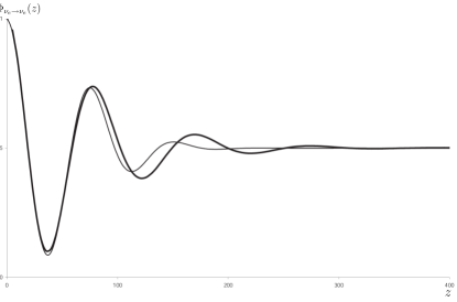
Figure 3: QFT flux (thick line) vs. standard formula (thin line) for $\theta=\pi/4$, $\sigma_{k}=10$, $m_{{}_{1}}=1$, $m_{{}_{2}}=3$, $Q=50$.

7 Summary

In this report we have discussed recent results in the area of field mixing and oscillations. We have shown that a consistent field theoretical treatment is possible, both for fermions and for bosons, once we realize the unitary inequivalence of the mass and flavor representations. The flavor Hilbert space is thus constructed and the flavor vacuum is shown to have the structure of a $SU(n)$ generalized coherent state, for the case of mixing among $n$ generations. We have then discussed the algebraic structure of the currents and charges associated with field mixing.

On the basis of these results, exact oscillation formulas have been calculated, exhibiting non-perturbative corrections with respect to the usual QM ones. The usual formulas are shown to be approximately valid in the relativistic region. Exact oscillation formulas in space can also be derived by use of the relativistic flavor currents.

We have also shown that a geometric phase is associated to flavor oscillations and discussed the role of the CP violating phase in connection with the algebra of currents associated to three flavor mixing.

For lack of space, we have omitted other interesting development, in particular we would like to mention the analysis, in the above framework, of the neutrino oscillations in matter (MSW effect) [37]. An interesting new line of research is the investigation of the issue of Lorentz invariance for the flavor states [38]: deformed dispersion relations for neutrino flavor states may be indeed incorporated into frameworks encoding the breakdown of Lorentz invariance [39].

References

• [1] T. Cheng and L. Li, Gauge Theory of Elementary Particle Physics, Clarendon Press, Oxford, 1989.
• [2] J. Davis, D. S. Harmer and K. C. Hoffmann, Phys. Rev. Lett. 20 (1968) 1205. M. Koshiba, in “Erice 1998, From the Planck length to the Hubble radius”, 170; S. Fukuda et al. [Super-Kamiokande collaboration], Phys. Rev. Lett. 86 (2001) 5656. Q. R. Ahmad et al. [SNO collaboration] Phys. Rev. Lett. 87 (2001) 071301; Phys. Rev. Lett.  89 (2002) 011301. K. Eguchi et al. [KamLAND Collaboration], Phys. Rev. Lett.  90 (2003) 021802 M. H. Ahn et al. [K2K Collaboration], Phys. Rev. Lett.  90 (2003) 041801
• [3] B. Pontecorvo, Zh. Eksp. Theor. Fiz. 33 (1958) 549; JEPT 6 (1958) 429; Z. Maki, M. Nakagawa and S. Sakata, Prog. Theor. Phys. 28 (1962) 870; V. Gribov and B. Pontecorvo, Phys. Lett.  B 28 (1969) 493; S. M. Bilenky and B. Pontecorvo, Phys. Rep. 41 (1978) 225.
• [4] R. Mohapatra and P. Pal, Massive Neutrinos in Physics and Astrophysics, (World Scientific, Singapore, 1991); J. N. Bahcall, Neutrino Astrophysics, (Cambridge Univ. Press, Cambridge, 1989).
• [5] V. Bargmann, Annals Math.  59 (1954) 1; A. Galindo and P. Pascual, Quantum Mechanics, (Springer Verlag, 1990).
• [6] D. M. Greenberger, Phys.  Rev. Lett. 87 (2001) 100405.
• [7] M. Zralek, Acta Phys. Polon.  B 29 (1998) 3925.
• [8] C. Giunti, C. W. Kim and U. W. Lee, Phys. Rev. D 45 (1992) 2414; C.W. Kim and A. Pevsner, Neutrinos in Physics and Astrophysics, Harwood Academic Press, Chur, Switzerland,1993.
• [9] M. Blasone and G. Vitiello, Annals Phys.  244 (1995) 283 [Erratum-ibid.  249 (1995) 363].
• [10] M. Blasone, P. A. Henning and G. Vitiello, in M.Greco Ed.“La Thuile 1996, Results and perspectives in particle physics”, INFN Frascati 1996, p.139-152 [hep-ph/9605335].
• [11] M. Blasone, P. A. Henning and G. Vitiello, Phys. Lett. B 451 (1999) 140; M. Blasone, in A.Zichichi Ed. “Erice 1998, From the Planck length to the Hubble radius” (World Scientific) p.584, [hep-ph/9810329].
• [12] M. Binger and C. R. Ji, Phys. Rev. D 60 (1999) 056005. C. R. Ji and Y. Mishchenko, Phys. Rev. D 64 (2001) 076004; Phys. Rev. D 65 (2002) 096015.
• [13] K. Fujii, C. Habe and T. Yabuki, Phys. Rev. D 59 (1999) 113003 [Erratum-ibid. D 60 (1999) 099903]; Phys. Rev. D 64 (2001) 013011.
• [14] K. C. Hannabuss and D. C. Latimer, J. Phys. A 36 (2003) L69; J. Phys. A 33 (2000) 1369.
• [15] M. Blasone and G. Vitiello, Phys. Rev. D 60 (1999) 111302.
• [16] M. Blasone, P. Jizba and G. Vitiello, Phys. Lett. B 517 (2001) 471.
• [17] M. Blasone, A. Capolupo and G. Vitiello, in Yue-Liang Wu, editor, Flavor Physics, 425-433. World Scientific, Singapore 2002. [hep-th/0107125];
• [18] M. Blasone, A. Capolupo, O. Romei and G. Vitiello, Phys. Rev. D 63 (2001) 125015.
• [19] M. Blasone, A. Capolupo and G. Vitiello, Phys. Rev. D 66 (2002) 025033;
• [20] M. Blasone and J. S. Palmer, [hep-ph/0305257]
• [21] M. Blasone, P. P. Pacheco and H. W. Tseung, Phys. Rev. D 67 (2003) 073011.
• [22] M. Blasone, P. Jizba and G. Vitiello, [hep-ph/0308009].
• [23] C.Itzykson and J.B.Zuber, Quantum Field Theory, (McGraw-Hill, New York, 1980);
• [24] H.Umezawa,Advanced Field Theory: Micro, Macro and Thermal Physics (American Institute of Physics, 1993)
• [25] A. Perelomov, Generalized Coherent States and Their Applications, (Springer–Verlag, Berlin, 1986).
• [26] M. Blasone, P. A. Henning and G. Vitiello, Phys. Lett.  B 466 (1999) 262;
• [27] Y. Aharonov and J. Anandan Phys. Rev. Lett. 58 (1987) 1593; Phys. Rev. Lett. 65 (1990) 1697.
• [28] X. B. Wang, L. C. Kwek, Y. Liu and C. H. Oh, Phys. Rev. D 63 (2001) 053003.
• [29] B. Kayser, Phys. Rev.  D 24 (1981) 110; B. Kayser, F. Gibrat-Debut and D. Perrier, The Physics of massive neutrinos, World Scientific, 1989.
• [30] M. Beuthe, Phys. Rev. D 66 (2002) 013003; Phys. Rep.  375 (2003) 105.
• [31] C. Giunti, JHEP 0211 (2002) 017. C. Giunti and C. W. Kim, Phys. Rev. D 58 (1998) 017301.
• [32] W. Grimus and P. Stockinger, Phys. Rev. D 54 (1996) 3414; W. Grimus, P. Stockinger and S. Mohanty, Phys. Rev. D 59 (1999) 013011.
• [33] C. Y. Cardall, Phys. Rev. D 61 (2000) 073006; C. Y. Cardall and D. J. H. Chung, Phys. Rev. D 60 (1999) 073012.
• [34] K. Kiers and N. Weiss, Phys. Rev. D 57 (1998) 3091.
• [35] T. Yabuki and K. Ishikawa, Prog. Theor. Phys. 108 (2002), 347.
• [36] B. Ancochea, A. Bramon, R. Munoz-Tapia and M. Nowakowski, Phys. Lett. B 389 (1996) 149.
• [37] K. Fujii, C. Habe and M. Blasone, [hep-ph/0212076].
• [38] M. Blasone, J. Magueijo and P. Pires-Pacheco, [hep-ph/0307205].
• [39] J. Magueijo and L. Smolin, Phys.  Rev. D 67 (2003) 044017; Phys. Rev. Lett. 88 (2002) 190403.