Constraints on Neutrino Parameters from Neutral-Current Solar Neutrino Measurements

Abstract

We generalize the pull approach to define the $\chi^{2}$ function to the analysis of the data with correlated statistical errors. We apply this method to the analysis of the Sudbury Neutrino Collaboration data obtained in the salt-phase. In the global analysis of all the solar neutrino and KamLAND data we find the best fit (minimum $\chi^{2}$) values of neutrino parameters to be $\tan^{2}\theta_{12}\sim 0.42$ and $\delta m_{12}^{2}\sim 7.1\times 10^{-5}$ eV². We confirm that the maximal mixing is strongly disfavored while the bounds on $\delta m_{12}^{2}$ are significantly strengthened.

As the solar neutrino physics moves from the discovery stage to the precision measurements stage increasingly more data are becoming available for a critical analysis. Several experimental groups recently announced new results. The Sudbury Neutrino Observatory (SNO) Collaboration announced results from the neutral-current measurements in the salt phase of the experiment yenisno . A new, very precise measurement of the astrophysical S-factor for the reaction ⁷Be(p,$\gamma$)⁸B was performed by the Seattle-TRIUMF group Junghans:2003bd , updating their previous result Junghans:2001ee .

Earlier SNO charged-current (CC) measurements Ahmad:2001an ; Ahmad:2002ka confirmed the deficiency in the solar neutrino flux and helped narrow the neutrino parameter space. Earlier SNO neutral-current (NC) measurements Ahmad:2002jz yielded a total (all flavors) ⁸B solar neutrino flux which is in very good agreement with the Standard Solar Model (SSM) predictions Bahcall:2000nu . In a parallel development the reactor antineutrino disappearance observed by the KamLAND Collaboration Eguchi:2002dm found to favor the same region of the neutrino parameter space (the so-called Large Mixing Angle (LMA) region) as the solar neutrino experiments. In a sense KamLAND and SNO are complementary experiments with KamLAND being more sensitive to the difference between squares of the neutrino masses, $\delta m^{2}$, and SNO providing increasingly more precise constraints on the mixing angle as well as $\delta m^{2}$.

The new SNO NC measurement is able to determine the total active solar neutrino flux in a model-independent way. In particular no assumptions need to be made about the energy dependence of the flux. This feature makes the new data very valuable in restricting SSM or neutrino properties.

In a previous paper Balantekin:2003dc we presented a global analysis of all the solar neutrino and KamLAND data using a covariance approach. The aim of this paper is to perform a similar analysis using the pull approach. We use the pull approach in the form proposed and implemented by Fogli et al Fogli:2002pt . Although the covariance and pull approaches are strictly equivalent, the pull approach seems to provide a treatment of statistical and systematic uncertainties which is more transparent, easier to implement, and computationally simpler. In our analysis we include correlations between statistical errors.

We now enumerate the changes we incorporated in this paper as compared with our previous global analysis. The calculations of neutrino propagation in matter are done as described in Ref. Balantekin:2003dc . Since the SNO Collaboration has not yet announced a live-time distribution for zenith angles, we used the live-time information previously provided in the SNO data page HOWTOSNO to calculate Earth regeneration effects and the 24-hour average neutrino survival probabilities. In our calculations we ignored experimental correlations between SNO’s data sets as recommended by the SNO Collaboration HOWTOSNO2 . They emphasized that even though treatment of these correlations require extensive knowledge of the SNO detector, they have very little impact on determining confidence level regions.

The data set used in this analysis includes the average rate of the gallium experiments (SAGE Abdurashitov:2002nt , GALLEX Hampel:1998xg , GNO Altmann:2000ft ), the total rate of the Homestake chlorine experiment Cleveland:nv , 44 data points from the 1496 days SK zenith-angle-spectrum Fukuda:2002pe , 34 data points from the 2002 SNO day-night-spectrum Ahmad:2002ka as well as the newly-released SNO NC, CC, and electron scattering (ES) data yenisno . We calculated the CC cross section using the effective field approach Butler:1999sv , with radiative corrections as described in Ref. Kurylov:2002vj . In our calculations we used the counter-term value of $L_{1A}=4.5$ fm³ Chen:2002pv ; Balantekin:2003ep . For new salt phase SNO data we calculated the detector-averaged cross-sections using updated detector response function given in Ref. yenisno and higher threshold of 5.5 MeV as described in the SNO data page HOWTOSNO2 . The NC, CC, and ES fluxes are added as new data points. The systematic correlations of these new measured NC, CC, and ES fluxes are taken into account as described in HOWTOSNO2 . The main systematic sources of errors, like energy scale, radial accuracy, isotropy mean, radial energy bias, internal background neutrons, neutron capture, etc. are taken into account with the appropriate correlation coefficients given in HOWTOSNO2 .

Following the suggestion of Ref. Bahcall:2002zh , we added cross section errors first linearly and then quadratically in the parts contributing to the low and high energy parts of for radiochemical experiments. This change in cross section treatment resulted in a slight reduction of the allowed region contours. SNO collaboration has provided a statistical correlation matrix for the salt phase. The analysis of Ref. Fogli:2002pt proves that for uncorrelated statistical errors the pull and covariance approaches yield identical $\chi^{2}$ values. In the Appendix we write down the appropriate relations when statistical errors are correlated and prove that Fogli et al. result can be generalized to the correlated statistical errors. In our calculations we used the SSM systematics and fluxes Bahcall:2000nu .

We calculated the theoretical CC flux using the prescription given in the SNO data page HOWTOSNO2 :

$$\frac{\int_{0}^{\infty}\int_{0}^{\infty}\int_{5.5}^{\infty}\phi_{SSM}(E_{\nu})P_{ee}\frac{d\sigma}{dT_{e}}(E_{\nu},T_{e})R(T_{e},T)dE_{\nu}dT_{e}dT}{\int_{0}^{\infty}\int_{0}^{\infty}\int_{5.5}^{\infty}\phi_{SSM}(E_{\nu})\frac{d\sigma}{dT_{e}}(E_{\nu},T_{e})R(T_{e},T)dE_{\nu}dT_{e}dT},$$ (1)

where $\phi_{SSM}$ is the SSM flux, $P_{ee}$ is the electron neutrino survival probability, and $R$ is the energy response function. This result was used to calculate the CC/NC double ratio (see e.g. Ref. Maris:2001tg ).

The collective effect of the fractional systematic errors of the SSM input parameters appear as a shift of the neutrino fluxes:

$$\Phi_{i}\rightarrow f_{i}\Phi_{i},$$ (2)

where the index $i$ represents the neutrino source (pp, ⁸B, etc.). The shift $f_{i}$ can easily be calculated in the pull method (cf. Eq. (16) of Ref. Fogli:2002pt ). In the covariance approach one can allow the ⁸B flux to float freely. The shift in the pull approach provides a similar, but not identical function.

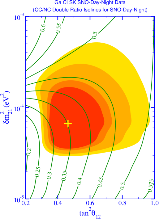
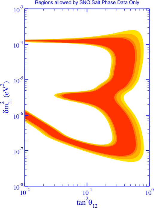
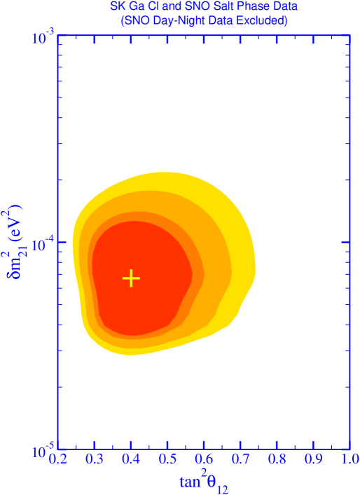
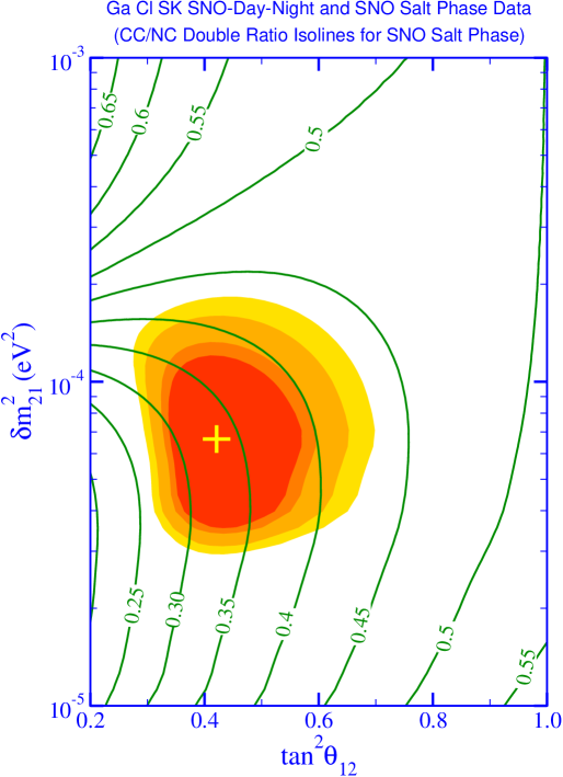
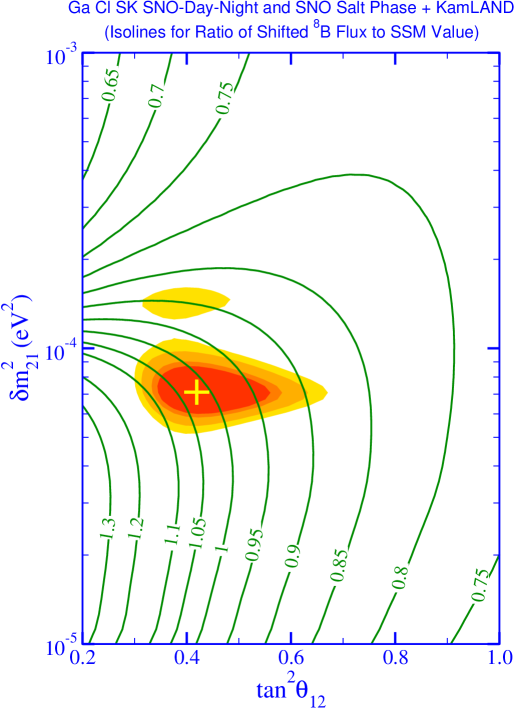
All graphs are shown with several confidence levels. In the figures shown the darkest shaded areas are the 90 % confidence level regions. Lighter shaded areas progressively include the 95 %, 99 %, and 99.73 % confidence level regions. In this manner, for example the entire shaded region in a given graph is the 99.73 % confidence level region. Best fit points are marked by a dagger. Isolines are clearly marked with corresponding values of the quantities which are being examined.

In order to compare the results before and after adding the SNO salt phase data, in Fig. 1 we show the LMA allowed region of solar neutrino parameter space. In this figure the CC/NC ratio isocountours, which are calculated for SNO experiment 2002 data with $T_{e,th}=5$ MeV, are also shown. At best fit (marked by a cross), the value of this ratio is $0.35$.

In Fig. 2 we show the allowed confidence levels in the neutrino parameter space using only the total NC, CC, and ES fluxes measured in the SNO salt phase measurement. This graph illustrates the crucial role of the additional spectrum information in constraining the neutrino parameters even after the neutral current measurements fix the ⁸B flux.

In Fig. 3 we show the allowed confidence levels in the LMA region of neutrino parameter space when chlorine, average rate of gallium experiments, SK zenith-spectrum and SNO salt phase measurement of NC, CC and ES data are used. In the calculations leading to this graph we excluded the SNO day-night spectrum data from 2002 in order to better understand the impact of new salt phase measurement. This figure can be compared to the Fig. 1. Fig. 3 uses the same input information as Fig. 1 except the SNO day-night information is replaced by the salt-phase results. Thus the relative impacts of the two data sets (salt-phase vs. day-night spectrum) in constraining the allowed neutrino parameter space are exhibited. Already the LOW solution is excluded at the 99.78 % confidence level. Clearly the information from the SNO salt phase helps significantly shrink the allowed region.

The global analysis of all available solar neutrino data is illustrated in Fig. 4. (This figure is similar to Fig. 3 except that the SNO day-night spectrum data are also included). We find the best fit (minimum $\chi^{2}$) values of neutrino parameters to be $\tan^{2}\theta_{12}\sim 0.42$ and $\delta m_{12}^{2}\sim 6.7\times 10^{-5}$ eV² from our combined analysis of all the solar neutrino data. Our minimum $\chi^{2}$ value is 70.5 for 83 data points and 2 parameters. The contours of the CC/NC ratio, which provides information about the electron neutrino survival probability, are also shown. Our best fit value for this ratio is $0.33$. This is in good agreement with the SNO value of $0.306\pm 0.026({\rm stat})\pm 0.024({\rm syst})$.

The global analysis of all available solar neutrino plus the KamLAND data are shown in Figs. 5 and 6. In Fig. 5 the ⁸B flux is fixed at the SSM value whereas in Fig. 6 it is taken as a free parameter. In Figure 5 we also show the ratio of this shifted ⁸B flux to the SSM value. The best fit of the shifted flux corresponds to 1.02 times the SSM value. In both graphs we find the best fit (minimum $\chi^{2}$) values of neutrino parameters to be $\tan^{2}\theta_{12}\sim 0.42$ and $\delta m_{12}^{2}\sim 7.1\times 10^{-5}$ eV². Even though the allowed regions of the neutrino parameter space are quite similar in shape, allowing the ⁸B flux float freely slightly enlarges the allowed region as one would expect.

In conclusion one observes that the new SNO NC, CC, and ES data fluxes are statistically correlated since they are derived from a single fit to the data. In this paper we applied the pull method generalized to incorporate correlated statistical experimental errors to the analysis of the SNO data. We confirm that the neutrino parameters are much better constrained after the addition of the SNO salt-phase data. In particular the maximal mixing is strongly disfavored while the bounds on $\delta m_{12}^{2}$ are significantly strengthened.

Pull Approach with Correlated Statistical Errors

Folllowing the notation of Fogli et al. Fogli:2002pt we designate the statistical errors for the observable $R_{n}$ by $u_{n}$, and the systematic error for the source $k$ for this observable by $c_{n}^{k}$. They also define scaled quantities

$$\Delta_{n}=\frac{R_{n}^{\mathrm{exp}}-R_{n}^{\mathrm{th}}}{u_{n}},$$ (3)

and

$$q^{k}_{n}=\frac{c^{k}_{n}}{u_{n}}.$$ (4)

Thus for the covariance approach one can write

$$\chi^{2}_{\mathrm{covar}}=\sum_{n,m}\Delta_{n}[\rho_{nm}+{\scriptstyle\sum_{k}}q_{n}^{k}q_{m}^{k}]^{-1}\Delta_{m},$$ (5)

where $\rho_{nm}$ is the statistical covariance matrix including the correlated errors. For the pull approach one has

$$\chi^{2}_{\mathrm{pull}}=\min_{\{\xi_{k}\}}\left[\sum_{n,m}(\Delta_{n}-{\scriptstyle\sum_{k}}q_{n}^{k}\,\xi_{k})\rho^{-1}_{nm}(\Delta_{m}-{\scriptstyle\sum_{k^{\prime}}}q_{m}^{k^{\prime}}\,\xi_{k^{\prime}})+\sum_{k}\xi^{2}_{k}\right],$$ (6)

where $\xi_{k}$ is the univariate Gaussian random variable introduced in the pull approach. Minimizing Eq. (6) with respect to $\xi_{k}$ we obtain

$$\xi_{k}=\sum_{h}S_{kh}\sum_{n,m}\rho^{-1}_{nm}\Delta_{m}q^{h}_{n},$$ (7)

where

$$S_{kh}=[\delta_{kh}+{\scriptstyle\sum_{n,m}}q_{n}^{k}\rho^{-1}_{nm}q_{m}^{h}]^{-1}\ .$$ (8)

Defining the matrices $B$ and $D$ through their matrix elements

$$B_{nm}=\sum_{h}q_{n}^{h}q_{m}^{h},$$ (9)

and

$$D_{nm}=\sum_{k,h}S_{kh}q_{n}^{h}q_{m}^{h},$$ (10)

one can show that the covariance matrix is $\rho+B$. Using the definition given in Eq. (10) it follows that the inverse of the covariance matrix is given by

$$(\rho+B)^{-1}=\rho^{-1}-\rho^{-1}D\rho^{-1}.$$ (11)

Substituting Eqs. (7) and (11) into Eqs. (5) and (6) after some algebra one gets

$$\chi^{2}_{\mathrm{covar}}\equiv\chi^{2}_{\mathrm{pull}}.$$ (12)

Figure 1: Allowed confidence levels in the LMA region of the neutrino parameter space when all solar neutrino experiments (chlorine, average of gallium, SNO and SK experiments) are included except the SNO salt phase data. CC/NC double ratio isolines for SNO experiment 2002 data also shown with $T_{e,th}=5$ MeV. At best fit (marked by a cross), the value of this ratio is $0.35$.

Figure 2: Allowed confidence levels in the neutrino parameter space from SNO salt phase measurement of NC, CC and ES only.

Figure 3: Allowed confidence levels in the LMA region of neutrino parameter space when chlorine, average rate of gallium experiments, SK zenith-spectrum and SNO salt phase measurement of NC, CC and ES included in the analyses. SNO day-night spectrum data from 2002 is not included in order to better understand the impact of the new salt phase measurement. Note that LOW solution is not allowed at 99.73% C.L. in this analysis (not shown). The best fit is marked by a cross.

Figure 4: Allowed confidence levels of neutrino parameter space when all available solar neutrino data (chlorine, average gallium, SNO and SK spectrums and SNO salt phase data) included in the analyses. CC/NC double ratio isolines for SNO Salt Phase data are also shown with $T_{e,th}=5.5$ MeV. At best fit (marked by a cross), the value of this ratio is $0.33$.

Figure 5: Allowed confidence levels from the joint analysis of all available solar neutrino data (chlorine, average gallium, SNO and SK spectra and SNO salt phase) and KamLAND reactor data The isolines for ratio of the shifted ⁸B flux (as described in the text) to the SSM value also superimposed on the plot. At best fit (marked by a cross) the value of this ratio is $1.02$.

Figure 6: Same as the previous figure, except ${}^{8}B$ flux is treated as a free parameter. Note that, shape of higher confidence levels look more similar to the original analyses of SNO Collaboration in which ${}^{8}B$ is treated as a free parameter as well.

References

- (1) S. N. Ahmed et al. [SNO Collaboration], arXiv:nucl-ex/0309004.
- (2) A. R. Junghans et al., arXiv:nucl-ex/0308003.
- (3) A. R. Junghans et al., Phys. Rev. Lett. 88, 041101 (2002) [arXiv:nucl-ex/0111014].
- (4) Q. R. Ahmad et al. [SNO Collaboration], Phys. Rev. Lett. 87, 071301 (2001) [arXiv:nucl-ex/0106015].
- (5) Q. R. Ahmad et al. [SNO Collaboration], Phys. Rev. Lett. 89, 011302 (2002) [arXiv:nucl-ex/0204009].
- (6) Q. R. Ahmad et al. [SNO Collaboration], Phys. Rev. Lett. 89, 011301 (2002) [arXiv:nucl-ex/0204008].
- (7) J. N. Bahcall, M. H. Pinsonneault and S. Basu, Astrophys. J. 555, 990 (2001) [arXiv:astro-ph/0010346].
- (8) K. Eguchi et al. [KamLAND Collaboration], Phys. Rev. Lett. 90, 021802 (2003) [arXiv:hep-ex/0212021].
- (9) A. B. Balantekin and H. Yuksel, J. Phys. G 29, 665 (2003) [arXiv:hep-ph/0301072].
- (10) G. L. Fogli, E. Lisi, A. Marrone, D. Montanino and A. Palazzo, Phys. Rev. D 66, 053010 (2002)[arXiv:hep-ph/0206162].
- (11) SNO Collaboration, Data Page, http://www.sno.phy.queensu.ca/sno/prlwebpage
- (12) SNO Collaboration, Data Page, http://www.sno.phy.queensu.ca/sno/results-09-03/howto.ps
- (13) J. N. Abdurashitov et al. [SAGE Collaboration], J. Exp. Theor. Phys. 95, 181 (2002) [Zh. Eksp. Teor. Fiz. 122, 211 (2002)] [arXiv:astro-ph/0204245].
- (14) W. Hampel et al. [GALLEX Collaboration], Phys. Lett. B 447, 127 (1999).
- (15) M. Altmann et al. [GNO Collaboration], Phys. Lett. B 490, 16 (2000) [arXiv:hep-ex/0006034].
- (16) B. T. Cleveland et al., Astrophys. J. 496, 505 (1998).
- (17) S. Fukuda et al. [Super-Kamiokande Collaboration], Phys. Lett. B 539, 179 (2002) [arXiv:hep-ex/0205075].
- (18) M. Butler and J. W. Chen, Nucl. Phys. A 675, 575 (2000) [arXiv:nucl-th/9905059]; M. Butler, J. W. Chen and X. Kong, Phys. Rev. C 63, 035501 (2001) [arXiv:nucl-th/0008032].
- (19) A. Kurylov, M. J. Ramsey-Musolf and P. Vogel, Phys. Rev. C 67, 035502 (2003) [arXiv:hep-ph/0211306].
- (20) J. W. Chen, K. M. Heeger and R. G. H. Robertson, Phys. Rev. C 67, 025801 (2003) [arXiv:nucl-th/0210073].
- (21) A. B. Balantekin and H. Yuksel, arXiv:hep-ph/0307227.
- (22) J. N. Bahcall, M. C. Gonzalez-Garcia and C. Pena-Garay, Phys. Rev. C 66, 035802 (2002) [arXiv:hep-ph/0204194].
- (23) M. Maris and S. T. Petcov, Phys. Lett. B 534, 17 (2002) [arXiv:hep-ph/0201087].