http://arXiv.org/abs/hep-ph/0309077
UNITU–THEP–12/03
NT@UW-03-22
HD-THEP-03-44
Analytic properties of the Landau gauge
gluon and quark propagators

Abstract

We explore the analytic structure of the gluon and quark propagators of Landau gauge QCD from numerical solutions of the coupled system of renormalized Dyson–Schwinger equations and from fits to lattice data. We find sizable negative norm contributions in the transverse gluon propagator indicating the absence of the transverse gluon from the physical spectrum. A simple analytic structure for the gluon propagator is proposed. For the quark propagator we find evidence for a mass-like singularity on the real timelike momentum axis, with a mass of 350 to 500 MeV. Within the employed Green’s functions approach we identify a crucial term in the quark-gluon vertex that leads to a positive definite Schwinger function for the quark propagator.

I Introduction

Dynamical chiral symmetry breaking and confinement are fundamental properties of QCD. In high energy processes such as deep inelastic scattering, quarks behave almost masselessly. However at low energies the observed hadron spectrum suggests that light quarks acquire large, dynamically generated masses through their interaction with the gauge sector of QCD. Quarks and gluons carry color charge and are not observed as asymptotic states, only occurring inside colorless bound states, the hadrons. The mechanism for such confinement in QCD is still not understood and it is not known whether a gauge invariant formulation even exists. However, in the framework of a quantum theory, physical degrees of freedom are necessarily subject to a probabilistic interpretation implying unitarity and positivity; the physical part of the state space of QCD should be equipped with a positive (semi-)definite metric. Therefore one way to investigate whether a certain degree of freedom is confined, is to search for positivity violations in the spectral representation of the corresponding propagator. Negative norm contributions to the spectral function signal the absence of asymptotic states from the physical part of the state space of QCD and are thus a sufficient (though not necessary) criterion for the confinement of the particle in question.

Neither confinement nor dynamical chiral symmetry breaking can be accounted for at any finite order in perturbation theory. These phenomena can only be explored in genuinely non-perturbative approaches such as those provided by lattice Monte–Carlo simulations (see e.g. Ref. Montvay:cy ; Rothe:kp ) and the Dyson–Schwinger, Green’s functions approach (see e.g. Refs. Alkofer:2000wg ; Roberts:2000aa ; Maris:2003vk ). Both approaches have their own strengths and weaknesses. Lattice simulations are the only ab initio calculations available so far. They contain the full non-perturbative structure of QCD but are limited by the enormous computational effort they require and by uncertainties in the infinite volume and continuum extrapolations that are needed to connect with the physical world. Furthermore, the implementation of small quark masses in most lattice simulations is computationally very expensive and, as yet, state-of-the-art calculations use light quark masses 6–10 times the physical values, thus necessitating a further extrapolation. On the other hand, the Dyson–Schwinger equations for the propagators of QCD are continuum-based and can be solved analytically in the infrared but must be truncated to obtain a closed, solvable system of equations vonSmekal:1997is ; Atkinson:1998tu ; Lerche:2002ep ; Zwanziger:2001kw . Recently, a concerted effort has been made to combine the strengths of these two approaches and quite definite statements on the infrared behavior of QCD have emerged Fischer:2002hn ; Fischer:2003rp ; Tandy:2003hn ; Bhagwat:2003vw . In this work we will apply a similar strategy to explore the analytic structure of the propagators of QCD from solutions in the spacelike Euclidean momentum region.

This paper is organized as follows: In Sec. II we briefly review the connection between positivity and confinement and outline the method we will use to investigate the analytic structure of the propagator in the timelike momentum region. In the third section we investigate positivity violation in the gluon and quark propagators which are obtained as solutions of Dyson–Schwinger equations in the truncation scheme of Refs. Fischer:2002hn ; Fischer:2003rp . We find clear evidence for positivity violations in the gluon propagator. The origin of these positivity violations is a branch point at $p^{2}=0$, followed by a cut along the real timelike axis. For the quark propagator we find no positivity violations as long as a certain non-perturbative Dirac structure is included in the quark-gluon vertex. This Dirac structure is dictated by the Ward–Takahashi identity in QED, and is also likely to exist in QCD because of the similar nature of the corresponding Slavnov–Taylor identity. In Sec. IV we seek parameterizations of the quark propagator. We investigate the ability of a number of meromorphic ansaetze to reproduce lattice data for the quark propagator. All the fits share the property of either a dominant real pole or a pair of complex conjugate poles very close to the real momentum axis. We also show that one can reproduce both the Dyson–Schwinger solutions and the lattice data by various parameterizations with branch point singularities, rather than poles. We give a summary of our results in the last section.

II Positivity and Confinement

One of the most intricate problems in quantum field theories is the separation of physical and unphysical degrees of freedom. In QCD this problem is directly connected with the issue of confinement, since we are searching for the mechanism which eliminates the colored degrees of freedom from the physical subspace, $\mathcal{V}_{phys}$, of the state space of QCD. In order to ensure a probabilistic interpretation of the quantum theory, $\mathcal{V}_{phys}$ is required to be positive semi-definite, whereas the total state space of QCD in covariant gauges has an indefinite metric.

A possible definition of a positive definite subspace, $\mathcal{V}_{phys}$, is given in the framework of the Kugo–Ojima confinement scenario Kugo:1979gm . Assuming the existence of a well-defined BRST charge operator, $Q_{B}$, the space of physical states is defined by

$${\mathcal{V}_{phys}}={\left\{|phys\rangle:Q_{B}|phys\rangle=0\right\}}.$$ (1)

Given the assumption of a well-defined, i.e. unbroken, global color charge, $Q^{a}$, it has been shown that the physical state space $\mathcal{V}_{phys}$ only contains color singlets, i.e. $\langle phys|Q^{a}|phys\rangle=0$ Kugo:1979gm ; Nakanishi:qm . In Landau gauge this assumption, the Kugo–Ojima confinement criterion, can be translated into the requirement that the ghost propagator should diverge more strongly than a simple pole at zero momentum Kugo:1995km .

In this scenario, longitudinal gluons as well as ghosts are removed from the physical spectrum of QCD by the BRST quartet mechanism (see e.g. Ref. Nakanishi:qm ). The colored states are BRST-quartet states, consisting of two parent and two daughter states of respectively opposite ghost numbers. The latter states are BRST-exact and thus BRST-closed (due to the nilpotency of the BRST transformation). The BRST daughters are orthogonal to all other states in the positive definite subspace and thus do not contribute to physical $S$-matrix elements. The parent states belong to the indefinite metric part of the representation space and are thus expected to violate positivity. Members of the elementary quartet related to gauge fixing are the ghosts, the antighosts and longitudinal gluons.

As the two parent states of a quartet belong to the indefinite metric part of the complete representation space, violation of positivity would provide evidence for the correctness of the Kugo–Ojima picture. E.g. positivity violation for transverse gluons indicates that transverse gluons are BRST-parent states with gluon-ghost states as daughters. The corresponding parents of opposite ghost number are gluon-antighost states with a mixture of gluon-ghost-antighost and 2-gluon states as daughters. A similar construction for quarks would consider quarks as BRST-parent states with quark-ghost states as daughters, and correspondingly, quark-antighost states as second set of parents and a mixture of quark-ghost-antighost and quark-gluon states as second type of daughter states. Thus an investigation of (non-)positivity of transverse gluons and quarks allows us to understand in more detail confinement via the BRST quartet mechanism

In order to complete the proof of confinement in this scenario one must still demonstrate the appearance of a mass gap in $\mathcal{V}_{phys}$ and the violation of cluster decomposition (see e.g. Ref. Strocchi:ci ; Nakanishi:qm and references therein) for colored states. Both requirements are related to the area law in the Wilson loop and, correspondingly, to a non-vanishing string tension in the quark-antiquark potential.

At this point we note that the basic assumption of the Kugo–Ojima confinement scenario still seems far from being proved: BRST-symmetry is a perturbative concept and it is not clear whether the symmetry remains unbroken in non-perturbative QCD vanBaal:1997gu . Furthermore, although clear evidence for a linearly rising potential between static quarks has been found in quenched lattice simulations (see Ref. Greensite:2003bk and references therein), a mathematical proof of a violation of cluster decomposition is not at hand. Nonetheless, the Kugo–Ojima confinement criterion in its Landau gauge formulation has been tested in Dyson–Schwinger studies and in lattice simulations. Both methods agree very well even on a quantitative level and find a strongly diverging ghost propagator at small momenta Suman:1996zg ; Langfeld:2002dd ; Furui:2003jr ; Alkofer:2000wg ; Fischer:2002hn ; Fischer:2003rp .

The Kugo–Ojima scenario is one particular mechanism that ensures the probabilistic interpretation of the quantum theory. However, even if it were eventually shown not to be appropriate, it is apparent that there is some mechanism which singles out a physical, positive semi-definite subspace in QCD. This suggests another criterion for confinement, namely violation of positivity. If a certain degree of freedom has negative norm contributions in its propagator, it cannot describe a physical asymptotic state, i.e. there is no Källén–Lehmann spectral representation for its propagator.

Within the framework of a Euclidean quantum field theory (which is used throughout this work) positivity is formulated in terms of the Osterwalder–Schrader axiom of reflection positivity Osterwalder:1973dx . (For a thorough mathematical formulation of the axiom the reader is referred to Refs. Haag:1992hx ; Glimm:ng ). In the special case of a two-point correlation function, $\Delta(x-y)$, the condition of reflection positivity can be written as

$$\int d^{4}x\;d^{4}y\;\bar{f}(\vec{x},-x_{0})\;\Delta(x-y)\;{f}(\vec{y},y_{0})\;\geq 0\;,$$ (2)

where $f(\vec{x},x_{0})$ is a complex valued test function with support in $\{(\vec{x},x_{0})\>:\>x_{0}>0\}$, i.e. for positive times. After a three-dimensional Fourier transformation, this condition implies

$$\int_{0}^{\infty}dt\;dt^{\prime}\;\bar{f}(t^{\prime},\vec{p})\;\Delta(-(t+t^{\prime}),\vec{p})\;f(t,\vec{p})\;\geq 0\,.$$ (3)

Provided there is a region around $t_{0}=-(t+t^{\prime})$ where $\Delta(t_{0},\vec{p})<0$, one can easily find a real test function $f(t)$ which peaks strongly at $t$ and $t^{\prime}$ and thereby demonstrate positivity violation. For the special case $\vec{p}=0$, the Osterwalder–Schrader condition, Eq. (3), can be given in terms of the Schwinger function, $\Delta(t)$, defined by

$$\Delta(t):=\int d^{3}x\int\frac{d^{4}p}{(2\pi)^{4}}e^{i(tp_{4}+\vec{x}\cdot\vec{p})}\sigma(p^{2})=\frac{1}{\pi}\int_{0}^{\infty}dp_{4}\cos(t\;p_{4})\sigma(p^{2}_{4})\;\geq 0\,,$$ (4)

where $\sigma(p^{2})$ is a scalar function extracted from the corresponding propagator. For the propagator of transverse gluons, $\sigma(p^{2})$ is simply given by the renormalization function times the tree-level expression $1/p^{2}$ (see Eq. (14) below) and we denote the corresponding Schwinger function by $\Delta_{g}(t)$. The quark propagator can be decomposed into a scalar and a vector part

$$S(p) =: ip\!\!\!/\,\sigma_{v}(p^{2})+\sigma_{s}(p^{2})\;,$$ (5)

leaving us with two scalar functions, $\sigma_{v}(p^{2})$ and $\sigma_{s}(p^{2})$, to form two Schwinger functions, $\Delta_{v}(t)$ and $\Delta_{s}(t)$.

Two simple examples for the analytic structure of a propagator in a quantum field theory are a real pole and a pair of complex conjugate poles. These highlight the paradigmatic behaviors of the Schwinger function, Eq. (4). In the following, we always discuss the propagators and the functions $\sigma_{s,v}(p^{2})$ in terms of the Lorentz invariant complex momentum, $p^{2}$. Our notation is such that positive real values, $p^{2}>0$, correspond to spacelike momenta.

(I) Real pole. The propagator of a real, massive, scalar particle has a single pole on the real timelike ($p^{2}<0$) momentum axis. In this case the propagator function is given by $\sigma(p^{2})=1/(p^{2}+m^{2})$ and it is easy to see from Eq. (4) that the Schwinger function decays exponentially,

$$\Delta(t)\sim e^{-m\;t}\,,$$ (6)

and is positive definite. For a bare propagator, the pole mass, $m$, is the same as the bare mass occurring in the Lagrangian. However, for an interacting particle, the pole mass can have both tree level and dynamically generated contributions. The real pole corresponds to the presence of a stable asymptotic state associated with this propagator. This does not imply that this state corresponds to an observable physical particle: provided the Kugo–Ojima scenario holds, all states belonging to a quartet representation of the BRST-algebra are excluded from the physical subspace, $\mathcal{V}_{phys}$, which contains only colorless singlets. Thus two-point correlations of colored fields may develop real poles in momentum space without contradicting confinement Oehme:1994pv . In lattice calculations Montvay:cy and other non-perturbative approaches HollenbergBurkardt , the exponential decay in Eq. (6) is used to extract hadron masses and other observables from the large time behavior of appropriate correlators.

(II) Complex conjugate poles. Another possible analytic structure for a propagator is a pair of complex conjugate poles with “masses” $m=a\pm ib$. As has been discussed in detail in Refs. Stingl:1996nk , such a propagator could describe a short lived excitation which decays exponentially at large timelike distances. Furthermore, it has been argued Stingl:1996nk that although causality is violated at the level of the propagators, the corresponding S-matrix remains both causal and unitary. Such complex conjugate poles lead to oscillatory behavior in the Schwinger function, $\Delta(t)$. Specifically,

$$\Delta(t)\sim e^{-a\;t}\>\cos(bt+\delta)\,.$$ (7)

In this case one has negative norm contributions to the Schwinger function and the effective mass,

$$m_{\rm eff}(t)=-\frac{d\ln\Delta(t)}{dt}$$ (8)

(defined in analogy to the real pole case, Eq. (6)) exhibits periodic singularities. Therefore the associated state (if there is any) must be an element of the unphysical subspace. Under the assumption of an unbroken BRST symmetry, this state must be a member of a BRST quartet, and the corresponding excitation is confined.

Complex conjugate poles have been found for the fermion propagators of QED₃ Maris:1995ns , QED₄ (see e.g. Atkinson:1978tk ), and QCD Bhagwat:2003vw ; Stainsby:1990fh ; Maris:1991cb ; Bender:1996bm ; Bender:1997jf ; Burden:1997ja in a variety of truncation schemes. In a number of these studies, the authors have discussed whether the observed positivity violations are genuine properties of the theory related to confinement or artifacts of the truncation schemes Maris:1995ns ; Stainsby:1990fh ; Krein:1990sf ; Burden:1991gd . As examined in the following section, it is our contention that dominant complex conjugate poles are indeed an artifact of the rainbow (bare vertex) truncation of the quark Dyson–Schwinger equation and that, at least in Landau gauge, confinement through positivity violation in the quark propagator is not manifest. Complex conjugate propagators are also known to be practicable in light-cone dominated processes Tiburzi:2003ja and have recently been investigated in terms of the solution of the Bethe–Salpeter equation Bhagwat:2003wu . It has also been suggested that the gluon propagator may have such an analytic structure Stingl:1996nk ; Gribov:1978wm ; Zwanziger:1991ac ; Driesen:1997wz . This possibility has been investigated in Refs. Hawes:ef ; Bender:1994bv .

Here, a note on positivity for the propagator of a Dirac field is in order. A dispersion relation representation of a fermion propagator in Minkowski space reads

$$S(p)=\int_{0}^{\infty}ds\frac{p\!\!\!/\,\rho_{v}(s)+\rho_{s}(s)}{p^{2}-s+i\epsilon}\;,$$ (9)

and positivity amounts to the requirements that for $s>0$

$$\rho_{v}(s)\geq 0\;,\qquad{\rm and}\qquad\sqrt{s}\;\rho_{v}(s)-\rho_{s}(s)\geq 0\;.$$ (10)

It is obvious that for a free Dirac field of mass $m$ one has

$$\rho_{v}(s)=\delta(s-m^{2})\;,\qquad{\rm and}\qquad\rho_{s}(s)=m\;\delta(s-m^{2})\;,$$ (11)

and thus $\sqrt{s}\rho_{v}(s)-\rho_{s}(s)=0$. For an interacting Dirac field with physical asymptotic states and mass $m$ one expects $\rho_{s,v}(s)=0$ for $s<m^{2}$. For $s>m^{2}$, Eq. (10) has to be satisfied. This requirement is automatically fulfilled if the stronger constraint

$$m\rho_{v}(s)\geq\rho_{s}(s)\,,$$ (12)

holds.

Given the linearity of the different types of integral transforms relating $\sigma_{s,v}(p^{2})$, $\rho_{s,v}(s)$, and $\Delta_{s,v}(t)$ to each other, one can conclude that $\sigma_{v}(p^{2})$ must be multiplied by a typical mass scale before being compared to $\sigma_{s}(p^{2})$. Thus, positivity violations can be signaled either in $\sigma_{v}(p^{2})$ alone, or in appropriate linear combinations of $\sigma_{v}(p^{2})$ and $\sigma_{s}(p^{2})$. We also consider the Schwinger function associated solely with $\sigma_{s}(p^{2})$, since it can be calculated with greater numerical accuracy. In general, oscillatory behavior in $\Delta_{s}(t)$ signals oscillatory behavior in $\Delta_{v}(t)$ as well.

Using the corresponding Schwinger functions, we can search for possible positivity violations and investigate the analytic structure of the gluon and quark propagators of QCD. The $t$-dependencies of these Schwinger functions are determined by the analytic properties of the propagator, and, for large $t$, are dominated by the singularity closest to $p^{2}=0$. A complementary, direct method of determining the analytic structure is to solve the corresponding Dyson–Schwinger equation over a large region of the complex momentum plane. However, from a numerical point of view, such a procedure is very expensive and is not feasible with the resources currently available to us. Furthermore, there is good evidence from an investigation of QED₃ that both methods agree very well Maris:1995ns . We are thus confident that the Fourier transformation method is able to determine the qualitative behavior of the propagators.

To complete this discussion we note that the conversion of a tree-level pole into an algebraic branch point with exponent larger than one is also known for certain approximations to the fermion propagator of QED₄ (see, e.g., supplement S4 in Ref. Jau76 and references therein). This type of singularity, $(p^{2}+m^{2})^{-1-\alpha/\pi}$, is related to the soft photon cloud. The examples discussed in this section (real poles, complex conjugate poles, or branch cuts) will form the basis of our investigation of the analytic structure for the quark and gluon propagators.

III Solutions of the propagator Dyson–Schwinger equations of Landau gauge QCD

In this section we present solutions of the coupled set of Dyson–Schwinger equations (DSEs) for the ghost, gluon, and quark propagators in Landau gauge and investigate some of their analytic properties. In order to keep this paper self-contained, we first briefly review the DSE truncation scheme developed in Refs. Fischer:2002hn ; Fischer:2003rp which is used to determine the propagators for Euclidean spacelike momenta, i.e. for real $p^{2}\geq 0$. It is important to note that the behavior of the propagators for $p^{2}\to 0^{+}$ is extracted analytically.

The DSEs for the quark, gluon and ghost propagators are derived from the QCD generating functional with gluon field configurations restricted to the first Gribov region Gribov:1978wm . In a recent work it has been argued that such a prescription is sufficient to eliminate the effects of Gribov copies from correlation functions Zwanziger:2003cf . Furthermore, the DSEs are not affected by imposing such a boundary condition on the generating functional of the gauge fixed theory because the Gribov horizon is a nodal surface for the integrand of this functional integral. Instead, the ghost two-point function has to satisfy the so-called horizon condition Zwanziger:2001kw , i.e. the ghost propagator has to diverge more strongly than a simple pole for $p^{2}\to 0^{+}$. This condition (which in Landau gauge is formally equivalent to the Kugo–Ojima confinement criterion discussed in the preceding section) turns out to be enforced by the ghost DSE Watson:2001yv ; Alkofer:2001iw ; Lerche:2002ep and is thus fulfilled by the DSE solutions in the truncation scheme that we employ.

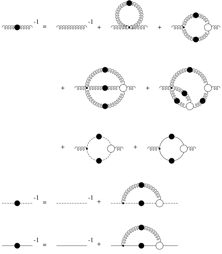
Figure 1: Diagrammatic representation of the Dyson–Schwinger equations for the gluon, ghost, and quark propagators. The wiggly, dashed, and solid lines represent the propagation of gluons, ghosts, and quarks, respectively. A filled blob represents a full propagator and a circle indicates a one-particle irreducible vertex.

A graphical representation of the DSEs for the ghost, gluon, and quark propagators is given in Fig. 1 and their full form can be found in Ref. Alkofer:2000wg . In Landau gauge (which is used throughout this work), the renormalized ghost, gluon and quark propagators, $D_{G}(p,\mu)$, $D_{\mu\nu}(p,\mu)$, and $S(p,\mu)$, respectively, are given in terms of scalar functions by

$$D_{G}(p,\mu) = -\frac{G(p^{2},\mu^{2})}{p^{2}}\,,$$ (13)

$$D_{\mu\nu}(p,\mu) = \left(\delta_{\mu\nu}-\frac{p_{\mu}p_{\nu}}{p^{2}}\right)\frac{Z(p^{2},\mu^{2})}{p^{2}}\,,$$ (14)

$$S(p,\mu) = \frac{1}{-ip\!\!\!/\,A(p^{2},\mu^{2})+B(p^{2},\mu^{2})}\>\>\>=:\>\>\>ip\!\!\!/\,\sigma_{v}(p^{2},\mu^{2})+\sigma_{s}(p^{2},\mu^{2})\,.$$ (15)

All these propagators are diagonal in their respective representations of SU($N_{c}$), so their color structure has been suppressed for simplicity. The dependence on the renormalization scale, $\mu$, is given explicitly for later use. Here, $G(p^{2},\mu^{2})$ and $Z(p^{2},\mu^{2})$ are the ghost and gluon dressing functions, respectively, and $A(p^{2},\mu^{2})$ and $B(p^{2},\mu^{2})$ are the vector and the scalar parts of the inverse of the quark propagator. The functions most relevant for our study of positivity are $Z(p^{2},\mu^{2})/p^{2}$, $\sigma_{s}(p^{2},\mu^{2})$ and $\sigma_{v}(p^{2},\mu^{2})$. Note that the ghost propagator trivially violates reflection positivity because of the way ghosts are introduced in Faddeev–Popov quantization Faddeev:fc .

Two renormalization-scale-independent combinations built from the scalar functions representing the different propagators are important for further discussion. First, $M(p^{2})=B(p^{2},\mu^{2})/A(p^{2},\mu^{2})$ denotes the renormalization-point-independent quark mass function. Second, as has been demonstrated in Ref. vonSmekal:1997is , a non-perturbative definition of the running coupling, is possible due to the non-renormalization of the ghost-gluon vertex in Landau gauge Taylor:ff . This results in the relation

$$\alpha(p^{2})=\alpha(\mu^{2})\>G^{2}(p^{2},\mu^{2})\>Z(p^{2},\mu^{2})\;.$$ (16)

In the following we investigate the full (unquenched) system of DSEs and also the quenched approximation to them in which quark loops are neglected, removing the back-reaction of the quarks on the ghost and gluon system.

III.1 Truncation scheme

Both the quenched and the unquenched system of ghost, gluon, and quark DSEs have been solved numerically in Refs. Fischer:2002hn ; Fischer:2003rp in a truncation scheme which neglects the effects of the four-gluon interaction and employs ansaetze for the ghost-gluon and the three-gluon vertices such that two important constraints are fulfilled: the running coupling, $\alpha(p^{2})$, is independent of the renormalization point and the anomalous dimensions of the ghost and gluon propagators are reproduced at the one-loop level for large momenta. In order to study the effects of violating gauge invariance by these truncation assumptions, the gluon DSE has been contracted with the one-parameter family of tensors

$${\mathcal{P}}^{(\zeta)}_{\mu\nu}(p)=\delta_{\mu\nu}-\zeta\,\frac{p_{\mu}p_{\nu}}{p^{2}}\,.$$ (17)

In Landau gauge, a violation of gauge invariance manifests itself in the appearance of spurious longitudinal terms in the gluon equation, which in turn introduces dependence of the ghost and gluon dressing functions on the parameter $\zeta$. The influence of these longitudinal terms has been examined in Ref. Fischer:2002hn by varying $\zeta$ and found to be surprisingly small. Further technical details of the truncation scheme in the Yang-Mills sector are relegated to Appendix A where we also discuss the dependence of our analysis on these details (see also Refs. Fischer:2002hn ; Fischer:2003rp ).

Employing asymptotic expansions for the propagators at small momenta, the untruncated ghost and gluon DSEs can be solved analytically for $p^{2}\to 0^{+}$ Watson:2001yv . One finds simple power laws, with exponents related as

$$Z(p^{2},\mu^{2}) \sim (p^{2}/\mu^{2})^{2\kappa}\;,$$ (18)

$$G(p^{2},\mu^{2}) \sim (p^{2}/\mu^{2})^{-\kappa}\;,$$ (19)

for the gluon and ghost dressing functions. The value of the exponent $\kappa$ depends somewhat on the details of the employed truncation scheme. In certain truncations it can be calculated analytically and it will depend on the parameter $\zeta$ Fischer:2002hn . The tensor ${\mathcal{P}}^{(\zeta=1)}_{\mu\nu}$ projects onto the purely transverse part of the gluon equation, and in this case the solution $\kappa=(93-\sqrt{1201})/98\approx 0.595$ has been found in Refs. Lerche:2002ep ; Zwanziger:2001kw . By varying $1\leq\zeta<4$, infrared solutions with exponents in the range $0.5<\kappa\leq(93-\sqrt{1201})/98$ have been shown to connect to numerical solutions for all momenta Fischer:2002hn . A recent infrared analysis of the ghost and gluon DSEs employing the most general ansatz for the ghost-gluon vertex suggests the exponent $\kappa$ is in the range $0.5<\kappa<1$ Lerche:2002ep (which is further restricted to $0.5<\kappa<0.7$ after constraints on the value of the running coupling are taken into account). A first attempt to include the two-loop diagrams in the gluon DSE also results in very similar values for the infrared exponent Bloch:2003yu and in Ref. Zwanziger:2003cf it has been shown that the two-loop diagrams have no effect on $\kappa$. Finally, exact renormalization group equations have recently been employed in a complementary investigation Pawlowski:2003hq of the infrared behavior of the gluon and ghost propagators with a resulting value for $\kappa$ in agreement with those above. These varied investigations all indicate that the Landau gauge gluon propagator vanishes as $p^{2}\to 0^{+}$ and predict an exponent $0.5<\kappa<0.7$.

For the subsequent discussion, it is important to note that the exponent $\kappa$ is very likely an irrational number. The relation of the exponents in Eqs. (18) and (19) results in an infrared finite strong coupling independent of the value of $\kappa$, c.f. Eq. (16). For transverse projection, the value is given by $\alpha(0)=8.915/N_{c}$.

The DSE for the quark propagator $S(p,\mu)$ is given by

$$S^{-1}(p,\mu)=Z_{2}(\mu^{2},\Lambda^{2})\,S^{-1}_{0}(p)+\frac{g^{2}}{16\pi^{4}}\,Z_{1F}(\mu^{2},\Lambda^{2})\,C_{F}\,\int^{\Lambda}d^{4}q\,\gamma_{\mu}\,S(q,\mu)\,\Gamma_{\nu}(q,p;\mu)\,D_{\mu\nu}(k,\mu)\,,$$ (20)

where $Z_{2}$ and $Z_{1F}$ are the quark wave function- and quark-gluon vertex-renormalization constants, respectively, and $\int^{\Lambda}$ represents a translationally-invariant regularization characterized by a scale, $\Lambda$. The momentum routing is $k=q-p$, and the factor $C_{F}=(N_{c}^{2}-1)/2N_{c}$ stems from the color trace of the loop.

In addition to the quark and gluon propagators, Eq. (20) involves the quark-gluon vertex, $\Gamma_{\nu}(q,p;\mu)$. This vertex is, in principle, determined by its own DSE Roberts:dr involving various ($n\leq 5$)-point correlators. However, the solution of such higher-order DSEs is difficult even in the simplest situations Detmold:2003au and we avoid the problem by making an ansatz for $\Gamma_{\nu}(q,p;\mu)$. As the structure of this vertex turns out to be crucial in our analysis of positivity violations in the quark propagator, we explore its construction in some detail.

A reasonable ansatz for the quark-gluon vertex has to satisfy at least two constraints: it should guarantee the multiplicative renormalizability of the quark propagator in the quark DSE, and it should at least approximately satisfy its non-Abelian Slavnov–Taylor identity. It has been shown in Ref. Fischer:2003rp that the construction

$$\Gamma_{\nu}(q,p;\mu)=V_{\nu}^{abel}(q,p;\mu)\,W^{\neg abel}(p^{2},q^{2},k^{2};\mu)\;,$$ (21)

with

$$W^{\neg abel}(p^{2},q^{2},k^{2};\mu) = G^{2}(k^{2},\mu^{2})\>\tilde{Z}_{3}(\mu^{2},\Lambda^{2})\;,$$ (22)

$$V^{abel}_{\nu}(q,p;\mu) = \Gamma_{\nu}^{CP}(q,p;\mu)$$ (23)

$$= \frac{A(p^{2},\mu^{2})+A(q^{2},\mu^{2})}{2}\gamma_{\nu}+i\frac{B(p^{2},\mu^{2})-B(q^{2},\mu^{2})}{p^{2}-q^{2}}(p+q)_{\nu}$$

$${}+\frac{A(p^{2},\mu^{2})-A(q^{2},\mu^{2})}{2(p^{2}-q^{2})}(p\!\!\!/\,+q\!\!\!/\,)(p+q)_{\nu}$$

$${}+\frac{A(p^{2},\mu^{2})-A(q^{2},\mu^{2})}{2}\left[(p^{2}-q^{2})\gamma_{\nu}-(p\!\!\!/\,-q\!\!\!/\,)(p+q)_{\nu}\right]$$

$$\hskip 99.58464pt\times\frac{p^{2}+q^{2}}{(p^{2}-q^{2})^{2}+(M^{2}(p^{2})+M^{2}(q^{2}))^{2}}\;,$$

and $\tilde{Z}_{3}$ being the ghost wave function renormalization constant, satisfies these requirements. Here it is assumed that the non-Abelian part of the vertex, $W^{\neg abel}(p^{2},q^{2},k^{2};\mu)$, can be factored out from the Dirac structure, and that the Dirac structure is given by $\Gamma_{\nu}^{CP}(q,p;\mu)$, the Curtis–Pennington (CP) construction of the fermion-photon vertex in QED₄ Curtis:1990zs ; Ball:ay . Note that the dressing of the longitudinal part of the CP vertex is dictated by the Abelian Ward identity

$$-ik_{\mu}\>\Gamma_{\mu}^{QED}(q,p;\mu)=S^{-1}(p,\mu)-S^{-1}(q,\mu)\;,$$ (24)

which results, among other things, in the appearance of a quark-gluon coupling term proportional to the sum of the incoming and outgoing quark momenta,

$$\Delta B_{\nu}:=i\frac{B(p^{2},\mu^{2})-B(q^{2},\mu^{2})}{p^{2}-q^{2}}(p+q)_{\nu}\,.$$ (25)

Such a coupling, being effectively scalar, may at first sight appear to violate chiral symmetry, as, in contrast to the perturbatively dominant vector coupling proportional to $\gamma_{\nu}$, the expression (25) commutes with $\gamma_{5}$. However, this scalar term only appears if chiral symmetry is already dynamically broken and is thus consistent with the chiral Ward identities. Its existence provides significant additional (self-consistent) enhancement of dynamical chiral symmetry breaking. Such a scalar coupling also appears in vertices that occur in systematic improvements on the rainbow (bare vertex) truncation Bender:2002as ; Bender:1996bb ; Hellstern:1997nv . This term will be important in our investigations of positivity below.

For comparison, we also employ a construction with a bare Abelian part of the vertex given by

$$V^{abel}_{\nu}(p,q;\mu) = Z_{2}(\mu,\Lambda)\>\gamma_{\nu}\,.$$ (26)

In both cases the input from the Yang-Mills sector of the theory, i.e. the factors from the dressed gluon propagator and the non-Abelian vertex dressing can be combined to give the running coupling $\alpha(k^{2})=g^{2}(\mu)\>G^{2}(k^{2},\mu^{2})\>Z(k^{2},\mu^{2})/4\pi$ according to Eq. (16). Thus we arrive at the truncated quark DSE

$$S^{-1}(p,\mu)=Z_{2}(\mu^{2})\,S^{-1}_{0}(p)+\frac{Z_{2}(\mu^{2})}{3\pi^{3}}\,\int d^{4}q\,\frac{\alpha(k^{2})}{k^{2}}\left(\delta_{\mu\nu}-\frac{k_{\mu}k_{\nu}}{k^{2}}\right)\gamma_{\mu}\,S(q,\mu)\,V_{\nu}^{abel}(q,p;\mu)\,.$$ (27)

In the quenched and unquenched calculations of the quark propagator we take $\alpha(k^{2})$ directly from the ghost and gluon equations.

We also consider the solutions of the quark DSE in the model calculations of Refs. Maris:1997tm ; Maris:1999nt ; Alkofer:2002bp . There, only the leading $\gamma_{\mu}$-part of the quark gluon vertex has been employed and the combination of the gluon and vertex dressing needed in the quark DSE has been modeled phenomenologically. With $\gamma_{m}=12/(11N_{c}-2N_{f})$ being the anomalous dimension of the quark propagator, we follow the authors of Ref. Maris:1999nt and use the model

$$\frac{\alpha(q^{2})}{q^{2}}=\frac{\pi}{\omega^{6}}D\,q^{2}\,e^{-q^{2}/\omega^{2}}+\frac{\pi\,\gamma_{m}\;[1-\exp(-q^{2}/m_{t}^{2})]}{q^{2}\;\frac{1}{2}\ln\left[e^{2}-1+(1+q^{2}/\Lambda^{2}_{QCD})^{2}\right]}\,,$$ (28)

with $\Lambda_{QCD}=0.234\;{\rm GeV}$ in the $\overline{\mbox{MS}}$-scheme, $N_{f}=4$ and the parameters $m_{t}=1.0\;\rm{GeV}$, $\omega=0.3\;\rm{GeV}$, and $D=0.781\;\rm{GeV}^{2}$ fixed by fitting the chiral condensate and pion decay constant. Omitting the perturbative logarithmic tail, we also compare with the model of Ref. Alkofer:2002bp , using a purely Gaussian interaction

$$\frac{\alpha(q^{2})}{q^{2}}=\frac{\pi}{\omega^{6}}D\,q^{2}\,e^{-q^{2}/\omega^{2}}\,,$$ (29)

with $\omega=0.5\;\rm{GeV}$ and $D=1\;\rm{GeV}^{2}$.

Despite the fact that these models for the effective interaction were designed to be used in combination with a bare vertex, we also use them in conjunction with the CP vertex, $\Gamma_{\nu}^{CP}$. By comparing quark propagators that result from employing either direct input from the ghost and gluon sector or the model forms, Eqs. (28) and (29), we are in a position to test whether the analytic properties of the quark propagator are more sensitive to the global strength of the quark-gluon interaction, to the overall shape of the (effective) running coupling, or to the details of the tensor structure of the quark-gluon vertex. First however, we will discuss the results of the numerical calculations for the gluon propagator.

III.2 Results for the gluon propagator for Euclidean momenta

     

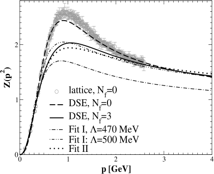
Figure 2: The solutionis of the quenched ($N_{f}=0$) and unquenched ($N_{f}=3$) coupled DSEs for the gluon dressing function, $Z(p^{2})$, are shown. The unquenched case with three massless flavors is compared to different fits (see text for details of the fits). In the left panel these are displayed on logarithmic scales, in the right panel, on linear scales. Results from quenched lattice calculations Bonnet:2001uh are given in the right panel.

In Fig. 2 we display the numerical results for the gluon dressing function calculated with zero (quenched) or three (unquenched) flavors of massless quarks and transverse projection, $\zeta=1$ (c.f. Eq. (17)), taken from Ref. Fischer:2003rp . In the diagram on the right of Fig. 2, the DSE results are compared to results from quenched lattice Monte–Carlo simulations Bonnet:2001uh . The quenched DSE results are seen to agree well with the lattice data. In contrast, the unquenched DSE gluon propagator is significantly suppressed in the intermediate momentum region where the screening effects of quark-antiquark pairs become important. For both $N_{f}=0$ and $3$, there are two qualitative properties that we can extract from these results: the analytically calculated infrared behavior given by Eq. (18), and a maximum around $\sim 1\;\rm{GeV}$, followed by relatively flat momentum dependence above this scale.

The behavior of the gluon dressing function in the infrared is captured by either of the irrational functions

$$Z^{ir}_{I}(p^{2}) = w_{I}\>\frac{(p^{2})^{2\kappa}}{(\Lambda^{2}_{I})^{2\kappa}+(p^{2})^{2\kappa}}\,,$$ (30)

$$Z^{ir}_{II}(p^{2}) = w_{II}\>\left(\frac{p^{2}}{\Lambda^{2}_{II}+p^{2}}\right)^{2\kappa}\,,$$ (31)

which are exact in the infrared limit (c.f. Eq. (18)) and which play a role when it comes to the interpretation of our results for the gluon Schwinger function, $\Delta_{g}(t)$. The value for the exponent $\kappa\simeq 0.595$ in these fits is taken from the infrared analysis of the DSEs. Note that for $\kappa\to 1$, the form of Eq. (30) becomes identical to the Gribov form proposed in Refs. Gribov:1978wm ; Zwanziger:mf . The normalization parameters $w_{I}$, $w_{II}$ and scales $\Lambda_{I}$, $\Lambda_{II}$ are chosen such that the Schwinger function of the ($\zeta=1,\,N_{f}=3$) numerical gluon propagator is reproduced by the Fourier transforms of the fits (the value of these parameters are given below). Our fits with these irrational functions $Z^{ir}_{I,II}(p^{2})$ are shown in Fig. 2 and clearly reproduce the behavior of the DSE gluon propagator for very small momenta but deviate significantly from the dressing functions at momenta above $\sim 400$ MeV.

To describe the behavior for larger momenta, we multiply the functions $Z^{ir}_{I,II}(p^{2})$ by a function incorporating the known ultraviolet behavior. To this end we note that in Ref. Fischer:2003rp the numerical running coupling has been fitted by

$$\alpha_{\rm fit}(p^{2})=\frac{\alpha(0)}{1+p^{2}/\Lambda^{2}_{QCD}}+\frac{4\pi}{\beta_{0}}\;\frac{p^{2}}{p^{2}+\Lambda^{2}_{QCD}}\;\left(\frac{1}{\ln(p^{2}/\Lambda^{2}_{QCD})}-\frac{\Lambda_{QCD}^{2}}{p^{2}-\Lambda_{QCD}^{2}}\right)\;.$$ (32)

In this expression the Landau pole has been subtracted as has been suggested in the framework of analytic perturbation theory Shirkov:1997wi . The value $\alpha(0)=8.915/N_{c}$ is known from the infrared analysis and $\beta_{0}=(11N_{c}-2N_{f})/3$. Using a MOM scheme and fitting only the ultraviolet behavior, a value $\Lambda_{QCD}=0.71\,\mbox{GeV}$ has been given in Ref. Fischer:2003rp .

Identifying $\Lambda_{I,II}=\Lambda_{QCD}$ for simplicity, we utilize the fits

$$Z_{I,\,II}(p^{2}) = Z^{ir}_{I,\,II}(p^{2})\;\alpha^{-\gamma}_{\rm fit}(p^{2})\;,$$ (33)

for further investigations, using the one-loop value of the gluon anomalous dimension, $\gamma=(-13N_{c}+4N_{f})/(22N_{c}-4N_{f})$. The quality of these fits can be seen in Fig. 2. For a discussion of the parameters used, see below.

     

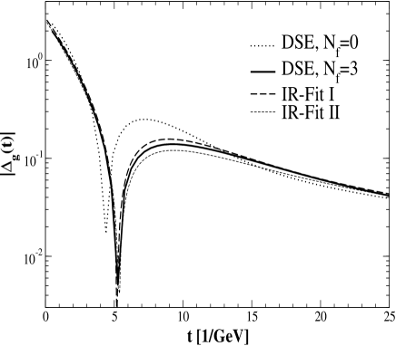
Figure 3: The results for the absolute value of the gluon Schwinger function, $\Delta_{g}(t)$, corresponding to our numerical results from the DSEs are shown and compared to the fits in the infrared (left panel) and the overall fits (right panel). The spikes mark the time scales where the Schwinger functions cross zero and negative norm contributions appear.

Employing a numerical Fourier transform routine, we can now calculate the Schwinger function, $\Delta_{g}(t)$ (defined by Eq. (4)), for the numerical solutions of the gluon DSE and for the various fits. The absolute values of the numerical Schwinger functions for $N_{f}=0,\,3$ (using transverse projection $\zeta=1$) are displayed in Fig. 3. The spikes mark the time scales at which the Schwinger functions cross zero and negative norm contributions appear in each gluon propagator. One notes that the Schwinger function in the quenched approximation differs visibly from that for three flavors, despite the similarity of the corresponding gluon dressing functions for Euclidean momenta Fischer:2003rp . In particular, the typical time scale, marked by the zero of the Schwinger function, decreases from $5.2\;{\rm GeV}^{-1}$ to $4.4\;{\rm GeV}^{-1}$. We have also explicitly checked that different choices for the projection of the gluon equation and other minor details of the truncation scheme lead only to minor quantitative alterations (see Appendix A). All gluon Schwinger functions we have calculated from the results of the coupled DSEs show the same qualitative behavior, thus demonstrating that neither the details of the projection in the gluon equation nor the feedback of (a small number of) dynamical quarks have any significant influence on the overall analytic structure of the gluon propagator. We clearly observe positivity violations in the gluon propagator. This is the first major result of this work.

III.3 Analytic structure of the gluon propagator

In the following we aim at an interpretation of our results in terms of the analytic structure of the gluon propagator in the timelike momentum region. As a first step we demonstrate that the infrared behavior of the gluon propagator, i.e. the behavior for $p^{2}\to 0^{+}$, is responsible for the non-trivial analytic structure. To this end, in the left-hand side of Fig. 3 the numerical results for the gluon Schwinger function (with $\zeta=1,\,N_{f}=3$) are compared to the infrared fits, Eqs. (30) and (31). The fitted parameters are $w_{I}=2.5$, $\Lambda_{I}=400$ MeV for IR-fit I, Eq. (30), and $w_{II}=2.7$, $\Lambda_{II}=420$ MeV for IR-fit II, Eq. (31). As we observed earlier, the fits only agree with the numerical gluon dressing function in the infrared momentum region. Nevertheless, in Fig. 3 we see that the agreement of the numerical Schwinger function with the Fourier transforms of each of these fits is excellent. It appears that the details of the intermediate and large momentum behavior of the gluon propagator have little or no influence on the qualitative analytical structure of the propagator in the “near-by” timelike momentum regime. In particular, the change in curvature at the bump of the gluon dressing function at a scale of $\sim 1$ GeV is not an important feature in this regard. In fact the crucial property of the gluon propagator is that it goes to zero for vanishing momentum. This can be seen easily as the relation,

$$0=D(p=0)=\int{d^{4}x}\;D(x)\,,$$ (34)

(with $D(p)=Z(p^{2})/p^{2}$) implies that the propagator function in coordinate space, $D(x)$, must contain positive as well as negative norm contributions, with equal integrated strengths.

For fit I (Eq. (33)) we have used two parameter sets, $w_{I}=2.4$, $\Lambda_{QCD}=500$ MeV and $w_{I}=2.0$, $\Lambda_{QCD}=470$ MeV. The first parameter set fits the gluon renormalization function better (especially in the ultraviolet) and the second set is optimized to fit the Schwinger function. For fit II (Eq. (33)) with the parameters $w_{II}=2.5$ and $\Lambda_{QCD}=510$ MeV both the gluon renormalization function and the Schwinger function are fitted very well. As the infrared fits I and II already reproduce the gluon Schwinger function it is no surprise that the complete fits, Eq. (33), do even better, see the right-hand side of Fig. 3. As already stated, for the sake of simplicity we have used only one common scale, $\Lambda_{QCD}$, for the infrared and ultraviolet behavior.

We are now in a position to deduce the possible analytic structure of the gluon propagator. We first observe that because of the infrared singularity of the ghost propagator, we expect a cut on the timelike momentum axis coming from the ghost-loop contribution to transverse gluons. As the ghost loop is the infrared dominant contribution in the gluon equation and therefore determines the infrared behavior of the gluon propagator, it is instructive to discuss the infrared fits to the gluon propagator first. The infrared fit I (Eq. (30)) contains a branch cut on the negative $p^{2}$ axis while the denominator contributes a pair of complex conjugate singularities at

$$p^{2}=\Lambda_{I}^{2}\>e^{\pm i\pi/(2\kappa)}\,.$$ (35)

The discontinuity across the negative $p^{2}$ axis is easily calculated. Writing $p^{2}_{\pm}=(-\rho\pm i\epsilon)\Lambda_{I}^{2}$ one obtains

$$\lim_{\epsilon\rightarrow 0}\left\{D_{I}(p^{2}_{+})-D_{I}(p^{2}_{-})\right\}\;=\;\frac{-2i\omega_{I}}{\Lambda_{I}^{2}}\;\frac{\sin(2\pi\kappa)\;\rho^{2\kappa-1}}{1+2\,\rho^{2\kappa}\,\cos(2\pi\kappa)+\rho^{4\kappa}}\,,$$ (36)

with $D_{I}(p^{2})=Z_{I}^{ir}(p^{2})/p^{2}$. This discontinuity rises from zero at $\rho=0$ to a maximum at the area of the pole locations and then rapidly decays as $\rho$ becomes larger.

In the infrared fit II (Eq. (31)) the numerator and the denominator conspire to produce one cut over $p^{2}\in(0,-\Lambda_{II}^{2})$. For the discontinuity we have (now for $p^{2}_{\pm}=(-\rho\pm i\epsilon)\Lambda_{II}^{2}$)

$$\lim_{\epsilon\rightarrow 0}\left\{D_{II}(p^{2}_{+})-D_{II}(p^{2}_{-})\right\}\;=\;\frac{-2i\omega_{II}}{\Lambda_{II}^{2}}\;\frac{\sin(2\pi\kappa)\;\rho^{2\kappa-1}}{(1-\rho)^{2\kappa}}\,,$$ (37)

with $D_{II}(p^{2})=Z_{II}^{ir}(p^{2})/p^{2}$ and for $0<\rho<1$ only. This rapidly diverges as $p^{2}\downarrow-\Lambda_{II}^{2}$ (i.e. $\rho\rightarrow 1$) and then drops discontinuously to zero: there is no discontinuity for $p^{2}<-\Lambda_{II}^{2}$.

Whereas the location of the singularity $p^{2}=-\Lambda_{II}^{2}$ in the infrared fit II is independent of the value of the exponent $\kappa$, the location of the complex conjugate singularities of IR-fit I as well as the magnitudes of the cuts in both fits depend on $\kappa$ and therefore on the truncation scheme. Although the exact value of $\kappa$ depends on the details of the truncation, various methods suggest that the exponent $\kappa$ is in the range $0.5<\kappa<1$ Lerche:2002ep ; Zwanziger:2001kw ; Fischer:2002hn ; Pawlowski:2003hq . It is exactly this range which corresponds to the pair of complex conjugate singularities in IR-fit I being located on the first Riemann sheet in the left half of the complex $p^{2}$-plane. In the limiting case $\kappa=0.5$, one obtains one real pole on the negative $p^{2}$-axis in both fits, and in the other limit, $\kappa=1$, IR-fit I corresponds to a pair of purely imaginary poles, i.e. exactly the form proposed in Refs. Gribov:1978wm ; Zwanziger:mf ; Stingl:1996nk .

To discuss the analytic structure of the full fits, Eq. (33), we must also look at the analytic properties of the expression for the running coupling, Eq. (32). The Landau pole at spacelike $p^{2}=\Lambda_{QCD}^{2}$ has been subtracted, so expression (32) only has singularities on the timelike real axis. The logarithm produces a cut on this half-axis, and the corresponding discontinuity vanishes for $p^{2}\to 0^{-}$, diverges at $p^{2}=-\Lambda_{QCD}^{2}$ and goes to zero for $p^{2}\to\infty$. In the fits I and II, Eq. (33), the running coupling (Eq. (32)) is raised to a non-integer power and multiplied by the infrared fits (Eqs. (30) and (31)). Thus, fit I also has a pair of complex conjugate singularities, at the same locations as those in Eq. (30). On the other hand, fit II has no non-analyticities other than the cut on the negative real axis. The discontinuity corresponding to the cut of the combination of the different factors in fit II is always positive, vanishes for $p^{2}\to 0^{-}$, diverges at $p^{2}=-\Lambda_{QCD}^{2}$ to $+\infty$ and falls to zero for $p^{2}\to-\infty$.

It is interesting to note the scale at which positivity violations occur. From Fig. 3 we determine that the zero crossing appears at $t\approx 5\;\mbox{GeV}^{-1}\approx 1\;\mbox{fm}$. This is roughly the size of a hadron and therefore the correct scale at which gluon screening should occur. One might speculate whether this represents an inherent, gauge invariant scale (as the locations of propagator poles are protected by Nielsen identities Nielsen:fs ), which is generated in the renormalization process. The pure power law $Z(p^{2})=(p^{2})^{2\kappa}$, which solves the system of DSEs in the case where the renormalization point $\mu$ is shifted to asymptotic values, is in perfect agreement with the scale-invariance of the underlying theory, corresponding to an infinite mass gap. Thus it is obvious that we can deduce the existence of a cut from the pure power laws, but we can not extract the related scale. This scale emerges from an interplay of infrared and ultraviolet properties of the theory, i.e. the transition of the gluon propagator from the infrared power law to its perturbative ultraviolet behavior.

Before concluding this subsection we comment on what lattice Monte–Carlo simulations say about positivity violation in the gauge boson propagator. For unquenched QCD, nothing is known because the gluon propagator has not yet been calculated with dynamical fermions. The pure Yang–Mills gauge propagator has been calculated on the lattice for almost twenty years following the pioneering work of Mandula and Ogilvie Mandula:rh , see e.g. Refs. Langfeld:2002dd ; Furui:2003jr ; Bonnet:2001uh ; lattice and references therein. However, explicit observations of positivity violation have been elusive as statistical errors and finite volume artefacts cloud the issue. Nevertheless, many hints of negative norm contributions in the gluon propagator have been reviewed in Mandula:nj . Clear measurements of positivity violation have been made for the case of $SU(2)$ Langfeld:2001cz and for the gluon propagator in three-dimensional Yang-Mills theory CucchieriPC .

Summarizing: the Landau gauge gluon propagator, as it results from the solution of coupled DSEs, displays positivity violations. This is in accordance with gluons being confined. The infrared behavior of the gluon propagator is analytically determined to be a power law. It has been demonstrated in Ref. Lerche:2002ep that this behavior is stable under a broad range of possible dressings of the ghost-gluon vertex. Furthermore, strong arguments have been presented in Ref. Zwanziger:2003cf for the existence of power laws in generalized truncations that include the four-gluon interaction. The power law behavior at small Euclidean momenta induces a cut on the real negative $p^{2}$-axis, as can be seen clearly from our infrared fits. It is this cut which causes the observed pattern of positivity violation. Fitting the gluon propagator for all Euclidean momenta and the corresponding Schwinger function we are able to describe the gluon propagator with fit II, Eq. (33), which has no singularities in the complex $p^{2}$-plane except for a cut on the negative real axis.

Note that this fit contains essentially two parameters: the overall magnitude which, because of renormalization properties, is arbitrary, and the scale $\Lambda_{QCD}$. The infrared exponent, $\kappa$, and the anomalous dimension of the gluon, $\gamma$, are not free parameters: $\kappa$ is determined from the infrared properties of the DSEs and the one-loop value is used for $\gamma$. Therefore, we have found a parameterization of the gluon propagator which has effectively only one physical parameter, the scale $\Lambda_{QCD}$. Combined with the relatively simple analytic structure of fit II, Eq. (33), this gives us confidence that we have succeeded in uncovering the most important features of the Landau gauge gluon propagator.

III.4 Results for the quark propagator

In Fig. 4 we display the mass function, $M(p^{2})=B(p^{2})/A(p^{2})$, and the wave function renormalization, $Z^{f}(p^{2})=1/A(p^{2})$ (note the superscript $f$ which differentiates this function from the gluon dressing function), of the quark propagator in the chiral limit, obtained from the coupled quark, ghost, and gluon DSEs Fischer:2003rp . We show quenched $(N_{f}=0)$ and unquenched $(N_{f}=3)$ results employing the generalized CP vertex, Eqs. (21)-(23). We also display the same functions calculated in the quenched approximation with the bare Abelian part of the quark gluon vertex, Eq. (26). On the Euclidean real axis, both vertex constructions lead to qualitatively similar but quantitatively quite different results. The bare vertex approximation does not give enough chiral symmetry breaking and is clearly disfavored by recent quenched lattice data Bonnet:2002ih ; Bowman:2002bm (also shown in Fig. 4). On the other hand, the results for the more elaborate vertex construction are well within the region suggested by the lattice calculations.

     

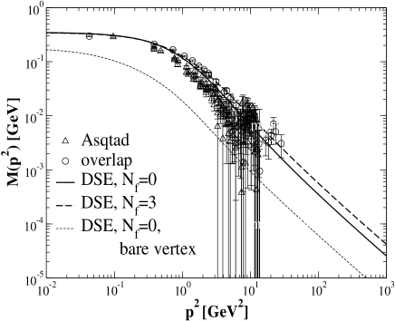
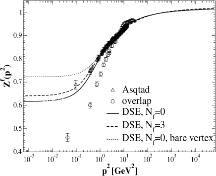
Figure 4: The quark mass function, $M(p^{2})$, and the wave function renormalization, $Z^{f}(p^{2})$, from quenched $(N_{f}=0)$ and unquenched ($N_{f}=3$ chiral quarks) DSEs Fischer:2003rp . Results for the generalized CP vertex, Eq. (23), and the bare vertex construction, Eq. (26), are compared with quenched lattice data in the overlap Bonnet:2002ih and Asqtad Bowman:2002bm formulations .

The quantitative difference between the DSE solutions using the bare vertex and the CP vertex turns into a qualitative difference for the corresponding Schwinger functions. The Fourier transformed scalar parts of the different quark propagators, $\Delta_{s}(t)$, are shown in Fig. 5. Similar results are obtained for the vector parts of the propagators, $\Delta_{v}(t)$, though they are numerically less accurate. As in the case of the gluon propagator, we plot the absolute values of the Schwinger functions on a logarithmic scale. The results in the left diagram are obtained employing the bare Abelian part of the vertex, Eq. (26). Clearly these solutions exhibit the oscillatory behavior of Eq. (7), which is characteristic for a propagator with a pair of complex conjugate “mass-like” singularities. A fit of the expression in Eq. (7) to our result gives the locations of these singularities as $m_{\hbox{\scriptsize sing}}=(209+101i)\;{\rm MeV}$.

A completely different picture is obtained from the Schwinger functions constructed using the CP vertex, Eq. (23), as can be seen in the diagram on the right of Fig. 5. Again we display results for the quenched case, $N_{f}=0$, and the case of $N_{f}=3$ chiral quarks. For $N_{f}=0$ we also make use of a fit to the running coupling as described in detail in Ref. Fischer:2003rp ; for all practical purposes the results are almost indistinguishable from those obtained with the numerical $\alpha(q^{2})$ as a solution of the ghost-gluon DSEs. We find no traces of negative norm contributions, and in all cases, a fit of the oscillatory form of Eq. (7) to our results indicates that there is a singularity (almost) on the real timelike axis, with an imaginary part of at most $8\%$ of its real part. The best fit is obtained for a real mass singularity at $m_{\hbox{\scriptsize sing}}=0.50\;{\rm GeV}$. For both the bare and the CP vertex, the deviation of the fits from the data at small time scales suggests that there is additional structure in the DSE solution which the simple pole fits (Eqs. (6) and (7)) do not capture. We shall investigate this in Sec. IV.

     

Figure 5: The left diagram displays the absolute value of $\Delta_{s}(t)$ employing the bare vertex construction in the quark DSE. The spikes correspond to zero crossings of the Schwinger function. These are absent in the diagram on the right where the results with the full CP vertex, Eq. (21), are considered. The chiral limit results are shown for $N_{f}=3$ and $N_{f}=0$, together with the fits to the Schwinger function of the quenched DSE solution. Furthermore we compare to a calculation with only the two most important terms of the quark-gluon vertex.

By turning the different contributions in the vertex construction of Eq. (23) on and off, we have identified the term which is responsible for the qualitative differences between the left and right diagram of Fig. 5. In addition to the (dominant) vector part of the vertex

$$\Sigma A_{\mu}:=\frac{A(p^{2})+A(q^{2})}{2}\gamma_{\mu}\,,$$ (38)

the presence of the scalar coupling $\Delta B_{\mu}$, Eq. (25), in the quark-gluon vertex is crucial for the substantial change in the analytic structure of the quark propagator compared to the truncation keeping only the vector part. Such a scalar term introduces additional feedback in the scalar self-energy, and its presence considerably enhances the amount of dynamical chiral symmetry breaking generated in the quark DSE. By varying the strength of this term compared to the leading $\Sigma A_{\mu}$-piece of the vertex, we find that a reduction of this term by about $20\%$ is enough to generate again positivity violations corresponding to dominant complex conjugate singularities.

	bare vertex	$\Sigma A_{\mu}+\Delta B_{\mu}$-term	CP vertex
YM $\alpha(k^{2})$, unquenched, $N_{f}=3$	0.21(1) $\pm$ 0.10(1) $i$	0.48(3)	0.50(3)
YM $\alpha(k^{2})$, quenched ($N_{f}=0$)	0.21(1) $\pm$ 0.10(1) $i$	0.48(3)	0.50(3)
fit A of Ref. Fischer:2003rp , quenched	0.209(4) $\pm$ 0.101(2) $i$	0.48(3)	0.50(3)
fit B of Ref. Fischer:2003rp , quenched	0.160(4) $\pm$ 0.076(2) $i$	0.42(3)	0.42(3)
Maris–Tandy model Maris:1999nt , Eq. (28)	0.55(1) $\pm$ 0.321(6) $i$	0.96(6)	1.1(1)
Gaussian model Alkofer:2002bp , Eq. (29)	0.53(1) $\pm$ 0.167(3) $i$	0.83(4)	0.83(6)
quenched QED (in units of $10^{-3}\Lambda$)	1.79(6) $\pm$ 0.43(2) $i$		1.51(9)

Table 1: Results for the fermion pole masses in the chiral limit for different interactions, as extracted from the behavior of the corresponding Schwinger functions. The quark masses are given in GeV, the QED₄ results are given in units of the UV cutoff $\Lambda$, and are obtained with $\bar{\alpha}=1.2$ for the bare vertex and $\bar{\alpha}=1.06$ for the CP vertex. The errors are estimates of the total numerical error; the numerical error in case of a real mass singularity is dominated by the fact that, on a logarithmic scale, the Schwinger functions are not perfect straight lines.

The question of positivity violation does not depend on the details of the input from the Yang–Mills sector of QCD. We obtain quantitatively similar results for the unquenched case with $N_{f}=3$ chiral quarks, for the quenched approximation with the running coupling taken directly from the Yang–Mills DSEs and for different models for the running coupling Fischer:2003rp . As a check, we also employ the model interactions given in Eqs. (28) and (29). Again we obtain evidence for a pair of complex conjugate singularities when a bare vertex is used and a singularity on the real timelike momentum axis once the additional scalar coupling is taken into account. Our results for the pole masses obtained in these models are given in Table 1. For the model interaction Eq. (28) we agree with the estimate for the singularity closest to $p^{2}=0$ given in Ref. Jarecke:2002xd based on a Taylor series expansion of the quark propagator functions, confirming that we can indeed extract the location of the first singularity via the Schwinger functions. Finally, we checked the truncation scheme of Ref. Bloch:2002eq where a model interaction with an infrared finite coupling has been employed together with a bare quark-gluon vertex. In this case we also found a pair of complex conjugate poles as could be expected.

Another interesting property of expression (25) is its insensitivity to explicit chiral symmetry breaking, i.e. a current quark mass. The contributions from current quark masses to the function $B(p^{2})$ are almost momentum independent and therefore cancel quite accurately in Eq. (25). The Schwinger functions become steeper with increasing quark mass, but show no signs of positivity violation, even for current quark masses as large as a few GeV. For a detailed comparison of the mass dependence of the Schwinger functions $\Delta_{s}(t)$ and $\Delta_{v}(t)$, we scale $\Delta_{v}(t)$ by the pole mass, $m_{\hbox{\scriptsize sing}}$ (extracted from the exponential decay of $\Delta_{s,v}(t)$), and plot $\Delta_{s}(t)$ and $m_{\hbox{\scriptsize sing}}\Delta_{v}(t)$ as function of the dimensionless variable $m_{\hbox{\scriptsize sing}}\,t$ in Fig. 6. This reveals that the only mass dependence is in the curvature of $\Delta_{s}(t)$ at small $m_{\hbox{\scriptsize sing}}\,t$: with increasing current quark mass the amount of curvature decreases.

     

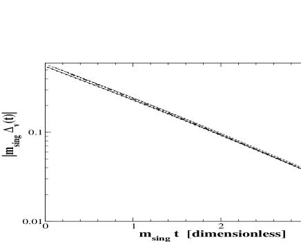
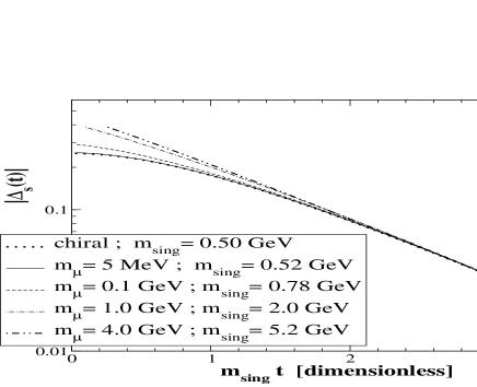
Figure 6: The dimensionless Schwinger functions $m_{\hbox{\scriptsize sing}}\Delta_{v}(t)$ (left) and $\Delta_{s}(t)$ (right) as function of $m_{\hbox{\scriptsize sing}}\,t$, where $m_{\hbox{\scriptsize sing}}$ is the “pole mass” as determined by the exponential decay of the Schwinger function for different current quark masses $m_{\mu}$, renormalized at $\mu=10\;{\rm GeV}$.

How can we understand this curvature that is present in $\Delta_{s}(t)$ but not in $\Delta_{v}(t)$? A possible origin could be the fact that the function $\sigma_{s}(p^{2})$ drops off like $1/q^{4}$ in the chiral limit while $\sigma_{v}(q^{2})$ decreases as $1/q^{2}$. As can be seen from Eq. (6), a single real pole on the negative momentum axis results in a pure, exponential decay of the corresponding Schwinger function. However, the Schwinger function of a propagator with two poles is

$$\frac{1}{\pi}\int_{0}^{\infty}dp\cos(tp)\frac{1}{p^{2}+m^{2}}\;\frac{1}{p^{2}+\Lambda^{2}}\;=\;\frac{1}{2(\Lambda^{2}-m^{2})}\left(\frac{1}{m}e^{-mt}-\frac{1}{\Lambda}e^{-\Lambda t}\right)\,,$$ (39)

and for $\Lambda$ somewhat larger than $m$, this could lead to the observed curvature at small $t$. This, in combination with the fact that this curvature tends to decrease with increasing current quark mass, suggests that this curvature is related to the $1/p^{2}$ fall off (up to logarithmic corrections) of $M(p^{2})$ in the chiral limit. However, there are other mechanisms that could generate such curvature as we will discuss in more detail in the next section.

Comparing the two panels of Fig. 6, we also see that $\Delta_{s}(t)$ approaches $m_{\hbox{\scriptsize sing}}\Delta_{v}(t)$ from below for all values of the current quark mass. In other words, we find that (within numerical accuracy) $m_{\hbox{\scriptsize sing}}\Delta_{v}(t)>\Delta_{s}(t)$ for all $t$. Based on the constraint for the spectral decomposition, Eq. (12), this is what one would expect for a propagator describing a Dirac field with asymptotic states. Thus, within this approach there are no signals of positivity violation in the non-perturbative quark propagator.

Considering these findings, we state the second major result of this work: the presence of a scalar quark-gluon coupling of sufficient strength leads to a positive definite quark propagator with a singularity on the timelike real momentum axis. As our quark-gluon vertex has been constructed as an ansatz, we do not have model independent information on the relative strength of the different tensor structures in the true quark-gluon vertex. Our assumption has been that all non-Abelian corrections can be accounted for by an overall factor multiplying an Abelian construction for the tensor structure of the vertex (see Eq. (21)). This factorization assumption has been tested in a recent investigation of the quark-gluon vertex in quenched lattice QCD and was found to be only valid at a qualitative level Skullerud:2003qu . However, as yet no definite statements can be extracted from the lattice calculations as they are only performed in two special kinematical situations, whereas in our calculations the vertex is probed over the whole range of momenta. Further investigations are necessary to determine the relative strength of the various components of the vertex in a model independent manner.

In QED₄ however, we encounter a somewhat different situation. The vertex construction is more constrained than in QCD as the longitudinal part of the CP vertex, the Ball–Chiu vertex Ball:ay , is exact and the relative strengths of the three longitudinal Dirac structures in the vertex are uniquely determined by the Ward identity, Eq. (24). The results for the fermion propagator in quenched approximation ($\alpha(q^{2})\equiv\overline{\alpha}$, constant) in the chirally broken phase of quenched QED are very similar to those of QCD. Again, we find a fermion propagator that satisfies positivity as long as it is calculated with a vertex obtained from the Ward identity but violates positivity if a bare vertex is used. The Schwinger functions are shown in Fig. 7 and the deduced (complex) pole masses are included in Table 1. Of course, it remains possible that the transverse parts of the exact vertex conspire to lead to positivity violation again. However, this is unlikely, in particular in QED where one has no confinement.

Figure 7: Results for two different vertex constructions in QED₄. For ease of comparison we employed two different values for the coupling, i.e. $\bar{\alpha}=1.2$ in the case of the bare vertex and $\bar{\alpha}=1.06$ for the case of the CP vertex.

IV Analytic properties of the quark propagator from parameterizations

In this section we explore the possible analytic structure of the quark propagator in more detail. Here we also consider the available lattice data for the quark propagator and investigate whether it is possible to obtain information on the analytic structure of the propagator by fitting this data, the DSE solutions, and the corresponding Schwinger functions with different parameterizations of pole locations and/or branch cuts. The singularity on the real momentum axis may be accompanied by additional real singularities at larger mass scaled or by complex conjugate singularities with a larger real part of the mass, or it may be the starting point of a branch cut on the negative real momentum axis. In the next two subsections we explore these possibilities.

IV.1 Meromorphic parameterizations

The most rigorous constraint on the non-perturbative quark propagator is that it must reduce to a free fermion propagator at large momenta because of asymptotic freedom. This entails that the propagator functions, $\sigma_{s,v}(p^{2})\stackrel{{\scriptstyle|p^{2}|\to\infty}}{{\longrightarrow}}0$ in all directions of the complex $p^{2}$-plane Oehme:1996ju . Additionally, the theory of complex functions tells us that if $\sigma_{v}(p^{2})$ and $\sigma_{s}(p^{2})$ are not constant, they cannot be analytic over the whole complex plane: non-constant, entire functions which are analytic at all finite points in the complex plane are already excluded by the asymptotic properties of the propagator functions. From the truncated set of DSEs explored in the previous section, we found the dominant (in terms of the Schwinger function) structure to be either a singularity on the negative real $p^{2}$ axis or a pair of complex conjugate singularities in the left half of the complex $p^{2}$-plane. In both scenarios the poles are accompanied by additional undetermined structures which are responsible for the small time behavior of $\Delta_{s}(t)$. Guided by these results we first consider parameterizations of the renormalized quark propagator using the meromorphic form

$$S(p)=Z_{2}^{-1}\sum_{j=1}^{n_{P}}\left(\frac{r_{j}}{ip\!\!\!/\,+a_{j}+ib_{j}}+\frac{r_{j}}{ip\!\!\!/\,+a_{j}-ib_{j}}\right)\,,$$ (40)

with $n_{P}$ pairs of complex conjugate poles located at $a_{j}\pm ib_{j}$ with residues $r_{j}$. This form includes the possibility of complex conjugate as well as purely real poles, but enforces neither of these from the outset. Similar simple parameterizations have been considered in Refs. Bhagwat:2003wu .

In the following, we use physical constraints as well as lattice data to fix the position of the various singularities. The only practical restriction on this procedure is in the number of parameters that can be pinned down. As further simplifications, we assume that the residues, $r_{j}$, of these poles are real (although this is not a strict requirement) and only consider the chiral limit.

For the propagator functions, $\sigma_{s}(p^{2})$ and $\sigma_{v}(p^{2})$, the form Eq. (40) simplifies to

$$\sigma_{v}(p^{2}) = Z_{2}^{-1}\sum_{j=1}^{n_{P}}\frac{2r_{j}(p^{2}+a_{j}^{2}-b_{j}^{2})}{(p^{2}+a_{j}^{2}-b_{j}^{2})^{2}+4a_{j}^{2}b_{j}^{2}}\,,$$ (41)

$$\sigma_{s}(p^{2}) = Z_{2}^{-1}\sum_{j=1}^{n_{P}}\frac{2r_{j}a_{j}(p^{2}+a_{j}^{2}+b_{j}^{2})}{(p^{2}+a_{j}^{2}-b_{j}^{2})^{2}+4a_{j}^{2}b_{j}^{2}}\,.$$ (42)

In terms of these quantities, we can construct the usual renormalization point independent mass function $M(p^{2})=\sigma_{s}(p^{2})/\sigma_{v}(p^{2})$ and the wave-function renormalization $Z^{f}(p^{2})=(p^{2}+M^{2}(p^{2}))\sigma_{v}(p^{2})$. In order to make contact with lattice data (where the finite lattice spacing leads to a maximum possible momentum), we renormalize at $\mu^{2}=16$ GeV².

There are various restrictions we can impose on the parameters $r_{j}$, $a_{j}$ and $b_{j}$ in the meromorphic form, Eq. (40). These arise from its mathematical properties, from experimental observables and from recent lattice data. Asymptotic freedom requires that quarks behave like free particles at large momenta. Consideration of the large momentum limit of $\sigma_{v}(p^{2})$ implies that

$$\sum_{j=1}^{n_{P}}r_{j}=\frac{1}{2}\,.$$ (43)

Since we are working in the chiral limit, the mass function, $M(p^{2})$, must vanish for large spacelike real momenta. This entails that

$$\sum_{j=1}^{n_{P}}r_{j}a_{j}=0\,.$$ (44)

Furthermore, $M(p^{2}\to+\infty)$ must be real and approach zero from above.

Asymptotically, the chiral limit mass function behaves as CONDENSATE

$$M(p^{2})\stackrel{{\scriptstyle p^{2}\to\infty}}{{\longrightarrow}}\frac{2\pi^{2}\gamma_{m}}{N_{c}}\frac{-\langle\bar{q}q\rangle}{p^{2}\left[\frac{1}{2}\ln(\frac{p^{2}}{\Lambda^{2}_{QCD}})\right]^{1-\gamma_{m}}}\,,$$ (45)

where $\langle\bar{q}q\rangle$ is the renormalization-point-invariant chiral condensate. Although the logarithmic behavior of Eq. (45) cannot be reproduced by these simple meromorphic fits, the logarithm is a slowly varying function and we estimate the condensate by fitting the mass function with Eq. (45) over the range $p^{2}\in(10^{3},10^{9})$ using the $\Lambda_{QCD}=0.5\;{\rm GeV}$ and the appropriate 1-loop value of $\gamma_{m}=12/33$ for $N_{f}=0$. We then insist that this condensate extracted from our meromorphic propagator agrees with the phenomenological value $\langle\bar{q}q\rangle=-[0.275(75)\,{\rm GeV}]^{3}$.

In order to be phenomenologically applicable, the propagator should reproduce the pion decay constant to a reasonable accuracy. To calculate this, we employ the approximation Roberts:dr ,

$$f_{\pi}^{2}\simeq Z_{2}\frac{N_{c}}{4\pi^{2}}\int_{0}^{\Lambda^{2}}dp^{2}p^{2}\frac{M(p^{2})}{Z^{f}(p^{2})}\left[\sigma_{v}(p^{2})\sigma_{s}(p^{2})+\frac{p^{2}}{2}\left(\frac{d\sigma_{v}(p^{2})}{dp^{2}}\sigma_{s}(p^{2})-\sigma_{v}(p^{2})\frac{d\sigma_{s}(p^{2})}{dp^{2}}\right)\right]\,,$$ (46)

which incorporates only the effects of the leading Dirac structure of the pion Bethe–Salpeter amplitude in the chiral limit. From a comparison of the relative sizes of the pion Bethe–Salpeter amplitudes in model calculations Maris:1997tm ; Alkofer:2002bp , one concludes that this approximation should lead to an underestimation of $f_{\pi}$ by 10-20 %. In our meromorphic fits we therefore demand that Eq. (46) gives $f_{\pi}\sim 0.08(3)$ GeV.

The Landau gauge quark propagator has been investigated on the lattice by a number of different groups using mean-field- and non-perturbatively- improved clover actions Skullerud:2000un , the Kogut–Susskind action Bowman:2002bm , the overlap formalism Bonnet:2002ih and the Asqtad quark action Bowman:2002bm . The data sets obtained in the latter two formulations have the smallest error bars and are therefore employed in what follows. Their mass functions and wave-function renormalizations have already been shown in Fig. 4. The mass function data from the lattice have been quadratically extrapolated Bonnet:2002ih ; Bowman:2002bm to the chiral limit, whereas the mass dependence of $Z^{f}(p^{2})$ is very mild so no extrapolation has been performed. While the simple extrapolation procedure that has been employed may lead to sizable errors Bhagwat:2003vw , it will prove sufficient for our purposes.

Unfortunately all of the lattice studies to date make use of the quenched approximation. Removing all internal quark loops is a potentially drastic modification of the theory. It destroys the unitarity of the S-matrix, however it is often assumed that these violations of unitarity are small. Strictly speaking, it is nonsensical to discuss the concept of positivity in such a situation and the lattice data discussed above cannot be relied on to provide any guidance in studying positivity of the quark propagator. However, from our experiences with the DSE studies of the previous section, one may expect that quenching will not qualitatively change the momentum dependence of the propagator (see Fig. 4). Additionally, the lattice data apparently still contain large finite volume effects (especially in the wave-function renormalization) Bowman:2002kn , and do not precisely constrain the asymptotic ($p^{2}\to+\infty$) behavior of the propagator . For these reasons we do not directly fit the lattice data (though a posteriori $\chi^{2}$ fits to it return very similar parameters to those we find below), but merely extract its three qualitative infrared features. Thus we assume that the zero momentum values of the mass function and wave-function renormalization, $M_{0}$ and $Z^{f}_{0}$, and an approximate width of the region of large dynamical mass generation, $\omega_{L}$ (defined by $M(\omega_{L}^{2})=M_{0}/2$), are robust against the effects of quenching (within substantial errors). With this in mind, we require that our parametric fits are in reasonable agreement with the extracted values of $M_{0}$, $Z^{f}_{0}$ and $\omega_{L}$. That is:

$$M_{0}=0.35(10)\>\mbox{GeV}\,,\quad\quad Z^{f}_{0}=0.6(2)\,,\quad\quad\omega_{L}=0.7(2)\>\mbox{GeV}\,.$$ (47)

Note that $\langle\bar{q}q\rangle$, $f_{\pi}$ and these three parameters are obviously not entirely unrelated.

Given the number of independent constraints we can impose, we can reasonably expect to be able to determine only five or six parameters. This implies $n_{P}\leq 3$ in Eq. (40). We find that three paradigmatic cases satisfy the requirements of Eqs. (43)–(47): three purely real poles (denoted, 3R), two pairs of complex poles (2CC), and a real pole plus a pair of complex conjugate poles (1R+1CC). In order to construct the best fits for each of these forms, we first impose the simple constraints of Eqs. (43) and (44) to reduce the number of parameters to be varied. Then for each parameterization we randomly sample the available parameter space, constructing a large ensemble of parameter sets that satisfy the full set of constraints. The best fit parameters and their errors are finally calculated as the mean and standard deviation of the parameters in this ensemble.

The simplest possible parameterizations of a single real pole or a single pair of complex conjugate poles ($n_{P}=1$ in Eq. (40)) cannot satisfy the required constraints. Specifically, enforcing the perturbative asymptotic behavior (Eqs. (43) and (44)) makes it impossible to satisfy any of the other requirements described above. Similarly, for two real poles ($n_{P}=2$, $b_{1}=b_{2}=0$), the restrictions on the infrared properties ($f_{\pi}$, $M_{0}$ and $\omega_{L}$) are incompatible with a realistic quark condensate.

	$r_{1}$	$a_{1}$ [GeV]	$b_{1}$ [GeV]	$r_{2}$	$a_{2}$ [GeV]	$b_{2}$ [GeV]	$r_{3}$	$a_{3}$ [GeV]
3R	0.365(15)	0.341(25)	–	1.2(8)	-1.31(12)	–	-1.06(*)	-1.40(*)
2CC	0.360(22)	0.351(69)	0.08(5)	0.140(*)	-0.899(*)	0.463(75)	–	–
1R+1CC	0.354(15)	0.377(64)	–	0.146(*)	-0.91(*)	0.45(7)	–	–

Table 2: Best fit parameters of the three meromorphic forms: three real poles (3R), two pairs of complex conjugate poles (2CC) and one real pole and one pair of complex complex conjugate poles (1R+1CC). The parameters whose errors are replaced by an asterisk, are completely determined in terms of the other parameters through Eqs. (43) and (44). In order to reproduce the results presented here, one should use the values that follow from Eqs. (43) and (44) for those constrained parameters.

	$M_{0}$ [GeV]	$Z^{f}_{0}$	$\omega_{L}$ [GeV]	$f_{\pi}$ [GeV]	$-\langle\bar{q}q\rangle^{1/3}$ [GeV]
3R	0.29(1)	0.55(7)	0.79(4)	0.071(3)	0.3(2)
2CC	0.33(11)	0.57(12)	0.69(27)	0.070(31)	0.3(3)
1R+1CC	0.31(7)	0.52(7)	0.72(25)	0.068(23)	0.3(2)

Table 3: Values for the various constrained quantities for the three parameterizations of Table 2. Errors are solely due to uncertainties in the parameterizations and do not include any additional systematic errors.

As mentioned above, a satisfactory realization of the requirements of Eqs. (43)–(47) is possible in the case of three real poles ($n_{P}=3$ and $b_{1}=b_{2}=b_{3}=0$). The best fit parameters we obtain are shown in Table 2 and related quantities that they result in are given in Table 3. Although the propagator functions $\sigma_{s,v}(p^{2})$ have poles at $p^{2}\sim-0.2\;\mbox{GeV}^{2}$, they exactly cancel in the combinations $M(p^{2})$ and $Z^{f}(p^{2})$. However the functions $M(p^{2})$ and $Z^{f}(p^{2})$ do have poles further in the timelike region, the first one occurring at $p^{2}\sim-0.75\;\mbox{GeV}^{2}$. Also the zeros of $Z^{f}(p^{2})$ on the real axis may be problematic as they will necessarily produce singularities in the CP construction of the quark-gluon vertex, c.f. Eq. (23).

In the case of two pairs of complex conjugate poles ($n_{P}=2$), the best fit parameters and calculated quantities are again given in Tables 2 and 3. Both $M(p^{2})$ and $Z^{f}(p^{2})$ exhibit unexpected behavior around $p^{2}\sim-0.12\;\mbox{GeV}^{2}$, where they have a very sharp pole and a zero on the real axis. This arises because $\sigma_{s}(p^{2})$ and $\sigma_{v}(p^{2})$ have zeros at very slightly differing momenta ($p^{2}=-0.127\;\mbox{GeV}^{2}$ vs $-0.117\;\mbox{GeV}^{2}$) and it may be somewhat troublesome. This behavior, as well as the small imaginary part of the location of the first pair of poles, suggests forcing the first pair of poles to collapse to one real pole ($n_{P}=2$, $b_{1}=0$).

Redoing the fits with one real pole and one pair of complex conjugate poles, we come up with very similar parameters to the 2CC parameterization, as listed in Table 2. The corresponding propagator functions are shown in Fig. 8. With this parameterization, the strange behavior of $M(p^{2})$ and $Z^{f}(p^{2})$ disappears and $Z^{f}(p^{2})$ only has complex conjugate poles and zeros ($Z^{f}(p^{2}=-0.41\pm 0.48i\;\mbox{GeV}^{2})=0$, $Z^{f}(p^{2}=-0.55\pm 0.69i\;\mbox{GeV}^{2})\to\infty$) so the longitudinal part of the quark-gluon vertex, Eq. (23) will not have particle-like singularities Roberts:2000hi . This parameterization also contains one parameter less than the others. Therefore we consider this to be the preferred form of the meromorphic parameterizations investigated here.

     

Figure 8: Propagator functions for the fit using one real pole and one pair of complex conjugate poles.

In comparing the three sets of parameterizations, it is worth remarking that the location of the (real part of the) first pole and its residue are extremely robust. The obtained value for this constituent quark mass, $m=377(64)\;{\rm MeV}$ for our best fit, is also in good agreement with a value extracted from lattice simulations of the quark propagator using a tree-level Symanzik improved action, $m=342(13)\;{\rm MeV}$ Karsch:1998xd . However, the constraints on the other features in the fits are less precise, especially in the case of three real poles. In Fig. 9 we compare the parameterizations given in Table 2 to the lattice data; overall, the agreement is quite acceptable. Note that the meromorphic fits have relatively low values of $Z^{f}_{0}$; this may change once finite volume effects are reduced in the lattice data. Also, each parameterization has a somewhat low value of $f_{\pi}$ in the chiral limit. This can be attributed on the one hand to the approximation leading to Eq. (46), and on the other hand to the approximations on the lattice: the chiral extrapolation as well as the omission of dynamical quarks might lead to an underestimation of $f_{\pi}$ in the lattice data Bhagwat:2003vw .

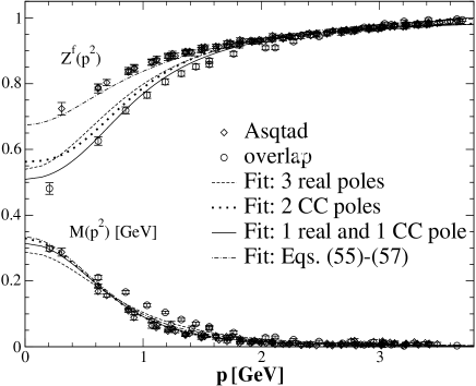
Figure 9: The best fit curves for the meromorphic parameterizations compared to the lattice data. For the details of the parameterization of $\sigma_{s,v}(p^{2})$ by a form with a branch cut, fitted to the Asqtad data, see the next subsection.

Having determined the best parameters for three different forms of our fit functions, we now examine the Fourier transforms of the momentum space propagator functions $\sigma_{s,v}(p^{2})$. Specifically, we attempt to determine whether the sub-dominant behavior of the various parameterizations can be determined from the Schwinger function, and, if so, apply this to the DSE solutions of Sec. III.

Using the identity

$$\int_{0}^{\infty}dx\frac{\cos(xy)}{x^{2}+c^{2}}=\frac{\pi}{2c}\exp(-c\,y)\quad\quad\quad\left[y\in\mathbb{R},\,\arg(c^{2})\neq\pi\right]\,,$$ (48)

we can directly calculate the Schwinger functions from our parameterizations (Eqs. (41) and (42)):

$$\Delta_{s}(t) = \sum_{i=1}^{n_{P}}sgn(a_{i})r_{i}e^{-|a_{i}|t}\cos(b_{i}t)\,,$$ (49)

$$\Delta_{v}(t) = \sum_{i=1}^{n_{P}}\frac{r_{i}e^{-|a_{i}|t}}{a_{i}^{2}+b_{i}^{2}}\left(|a_{i}|\cos(b_{i}t)-b_{i}\sin(b_{i}t)\right)\,.$$ (50)

For all parameterizations, the term with the smallest mass parameter $a_{i}$ will dominate for large $t$.

     

Figure 10: The Fourier-transform of both $\sigma_{s}(p^{2})$ (left) and $\sigma_{v}(p^{2})$ (right) for the optimal parameterizations with multiple poles. In the diagram on the left hand side we have included our DSE results.

In Fig. 10 we display the analytic Fourier transforms of the parameterized scalar and vector propagator functions, Eqs. (49) and (50). For comparison, we also include our DSE result for $\Delta_{s}(t)$ employing the CP vertex. Note the qualitative difference between the parameterization with two complex conjugate poles and the other two. Whereas the latter show no sign of positivity violation, in the 2CC parameterization we clearly see zero crossings of the Schwinger functions, both in $\Delta_{s}(t)$ and in $\Delta_{v}(t)$ (even a small imaginary component in the complex conjugate masses is detectable provided the Fourier transform can be calculated accurately to large enough $t$). Note that $\Delta_{s}(t)$ calculated from the meromorphic parameterizations shows a similar amount of small $t$ curvature to the DSE result, but $\Delta_{v}(t)$ is linear in this region. Thus multiple poles as explored here could explain the small $t$ behavior observed in the DSE Schwinger functions.

We also use these analytic Fourier transforms to test our numerical Fourier transform, finding that it reproduces the analytic results down to $\Delta_{s,v}(t)\sim 10^{-6}$ where we begin to run into accuracy problems. However, the numerical routine we employ is clearly able to distinguish between a dominant real pole and dominant complex conjugate poles. This gives us further confidence that our results from the DSE solutions in the previous section are not numerical artefacts.

IV.2 Parameterizations with branch cuts

As mentioned above, there is evidence that the Schwinger function $\Delta_{s}(t)$ is convex (with sizable curvature) at small $t$. On the other hand, the Schwinger function $\Delta_{v}(t)$ as obtained from the DSE solution shows no such curvature. This difference could be accommodated within the simple meromorphic fits of the previous subsection. However, this is certainly not the only possible mechanism leading to such a difference, and here we explore the consequences of allowing for singularities with branch cuts. As can be seen from Fig. 6, the curvature of $\Delta_{s}(t)$ depends on the current quark mass, so we also consider the effects of explicit chiral symmetry breaking.

Our motivation for investigating such parameterizations arises from considering the DSE for the quark propagator, Eq. (27). If the combination ${\alpha(k^{2})}/{k^{2}}$ is non-analytic at $k^{2}=(q-p)^{2}=0$ (in other words, if $\alpha(0)\neq 0$), the integration path necessarily passes through the external point $p$. Thus, in order to evaluate the quark propagator at arbitrary complex momenta, one has to deform the integration contour in the DSE and solve the DSE along this deformed integration path. As long as there are no singularities in the other factors of the integrand (i.e. in $S(q)$ and $V_{\nu}^{abel}(q,k)$), this can in principle be done unambiguously (though it is numerically a nontrivial task). However, if we want to evaluate the integral for a value $p$ at which the propagator, $S(p)$, has a singularity, we are forced by the analytic structure of $\alpha(k^{2})/{k^{2}}$ to include this value of $p$ in the integration contour for $d^{4}q$. Thus, we have a pinch singularity at this point coming from $S(q)$ and $\alpha(k^{2})/{k^{2}}$; this generally leads to a branch-cut, as is shown in more detail in Appendix B. We also note that the asymptotic form of the quark propagator has perturbatively calculable logarithmic contributions. Considering these points, we would expect that the singularities in $\sigma_{s,v}(p^{2})$ are branch points rather than simple poles. Thus we next attempt to parameterize the quark propagator by functions with branch cuts using the parameterization of the strong running coupling, Eq. (32), that has proven helpful in understanding the analytic structure of the gluon propagator.

As a first try, we shall fit the inverse propagator functions $M(p^{2})$ and $Z^{f}(p^{2})$ as obtained from the quark DSE with the CP vertex. Given the close agreement of the DSE solutions and the lattice quark propagator seen in Fig. 2, fitting the DSE solution will result in similar physical constraints to those of the previous subsection. The leading-order perturbative behavior is known, and we allow for one additional sub-leading term, that is to be fitted to the DSE solution. Furthermore, we want the parameterization to have a branch cut along the negative real axis starting at $p^{2}=-m_{\hbox{\scriptsize sing}}^{2}$. Thus we are lead to fit the DSE solutions with

$$Z^{f}(p^{2}) = Z_{2}\left(1-\frac{\alpha(p^{2}+m_{\hbox{\scriptsize sing}}^{2})}{2\pi}+\frac{C_{2}}{p^{2}+m_{\hbox{\scriptsize sing}}^{2}+\Lambda^{2}}\right)\,,$$ (51)

$$M(p^{2}) = C_{dcsb}\;\frac{\alpha(p^{2}+m_{\hbox{\scriptsize sing}}^{2})^{1-\gamma_{m}}}{p^{2}+m_{\hbox{\scriptsize sing}}^{2}+\Lambda^{2}}+\frac{C_{4}}{(p^{2}+m_{\hbox{\scriptsize sing}}^{2}+\Lambda^{2})^{2}}+C_{cqm}\;\alpha(p^{2}+m_{\hbox{\scriptsize sing}}^{2})^{\gamma_{m}}\,.$$ (52)

The parameters $C_{dcsb}$ and $C_{cqm}$ are related to the chiral condensate and the renormalized current quark mass, respectively:

$$-\langle\bar{q}q\rangle = C_{dcsb}\;\left(\frac{\pi\gamma_{m}}{2}\right)^{1-\gamma_{m}}\;\frac{N_{c}}{2\pi^{2}\gamma_{m}}\,,$$ (53)

$$m_{\mu} = C_{cqm}\;\alpha(p^{2}+m^{2})^{\gamma_{m}}\;\;\approx\;\;C_{cqm}\;\left(\frac{\pi\gamma_{m}}{\ln(p^{2}/\Lambda_{QCD}^{2})}\right)^{\gamma_{m}}\,.$$ (54)

The renormalization constant $Z_{2}$ is determined by the renormalization condition $Z^{f}(\mu^{2})=1$, $m_{\hbox{\scriptsize sing}}$ follows from the exponential decay of the Schwinger functions, and we take $\Lambda$ to be equal to $\Lambda_{QCD}$ in the running coupling, $\alpha(x)$, for which we use Eq. (32). The remaining free parameters in this fit, $C_{2}$ and $C_{4}$, are fitted to the numerical solution of the DSE and $\Lambda_{QCD}$ is also varied to improve this fit.

     

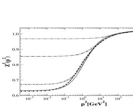
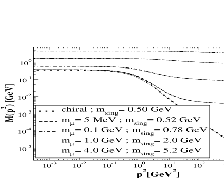
Figure 11: The functions $Z^{f}(p^{2})$ (left) and $M(p^{2})$ (right) obtained from parameterizations fitted to the numerical DSE solutions for different current quark masses. The solid curves are the fits (Eqs. (51) and (52)) and the dotted, dashed, and various dot-dashed curve are the DSE solutions as shown in the legend (the curves for $Z^{f}(p^{2})$ in the chiral limit and for $m_{\mu}=5\;{\rm MeV}$ are almost indistinguishable). The fit parameters are given in Table 4.

$m_{\mu}$	$C_{dcsb}$	$C_{4}$	$C_{cqm}$	$C_{2}$, $\tilde{C}$	$m_{\hbox{\scriptsize sing}}$
fitting $M$ and $Z^{f}$, Eqs. (51) and (52); $\Lambda_{QCD}^{2}=0.81\;{\rm GeV}^{2}$
DSE, chiral	0.086	0.248	0	-0.011	0.50
0.005	0.119	0.202	0.0074	-0.015	0.52
0.10	0.343	0	0.16	-0.067	0.78
1.0	0.36	0	1.65	-0.224	2.0
4.0	0	0	6.6	-0.348	5.2
fitting $\sigma_{s,v}$, Eqs. (55)–(57); $\Lambda_{QCD}^{2}=0.70\;{\rm GeV}^{2}$
DSE, chiral	0.086	0.234	0.0	1.27	0.50
0.005	0.10	0.234	0.0076	1.26	0.52
0.100	0.44	0	0.161	1.11	0.78
fitting $\sigma_{s,v}$, Eqs. (55)–(57); $\Lambda_{QCD}^{2}=0.50\;{\rm GeV}^{2}$
lattice, chiral	0.08	0.12	0.0	1.47	0.47
fitting $A$ and $B$, Eqs. (58)–(60); $\Lambda_{QCD}^{2}=0.70\;{\rm GeV}^{2}$
DSE, chiral	0.09	0.31	0	0.25	0.49
0.005	0.10	0.30	0.008	0.26	0.50
0.100	0.33	0	0.17	0.25	0.65
1.0	0.21	0	1.7	0.23	1.74
4.0	0	0	6.7	0.34	5.1

Table 4: Parameters for the various branch cut fits (Eqs. (51)–(60)) to the $N_{f}=0$ quark DSE solutions for different masses. A parameter set obtained by fitting Eqs. (55)–(57) to the Asqtad lattice data Bowman:2002bm is also included.

The results are shown in Fig. 11 for several different current quark masses representative of masses up to that of the bottom quark. The fitted parameters are given in the first section of Table 4. With only a few parameters, the fits represent the DSE solutions very well over the entire Euclidean region. The fitted values of $C_{cqm}$ are all reasonably close to the current quark masses that were used as input in the DSEs (small deviations are due to sub-leading effects) and the (fitted) chiral condensate is acceptable: $-\langle\bar{q}q\rangle=(290\;{\rm MeV})^{3}$.

Despite the fact that these parameterizations fit $Z^{f}(p^{2})$ and $M(p^{2})$ so well, the corresponding Schwinger functions do not fit the Schwinger functions of the DSE solutions. Clearly, the zeros of $p^{2}+M^{2}(p^{2})$ (which determine the poles of $\sigma_{s,v}(p^{2})$) will in general not occur on the negative $p^{2}$ axis when Eq. (52) is used for $M(p^{2})$. Indeed, the dominant singularities of the propagator functions $\sigma_{s,v}(p^{2})$ calculated from the parameterizations of $Z^{f}(p^{2})$ and $M(p^{2})$ are a pair of complex conjugate singularities, and the corresponding Schwinger functions clearly show oscillations (see Fig. 12). Extensive “fine-tuning” of the fitting form and/or the parameters is required in order for $p^{2}+M^{2}(p^{2})$ to have its first zero at the pole mass deduced from the Schwinger function of the DSE solution.

     

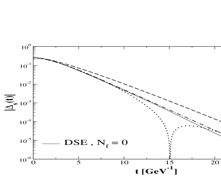
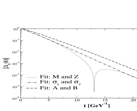
Figure 12: The Schwinger functions $\Delta_{s}(t)$ (left) and $\Delta_{v}(t)$ (right) for the three parameterizations with branch cuts, in the chiral limit. For comparison, we have also included our DSE results.

As a second alternative, we can directly parameterize $\sigma_{s,v}(p^{2})$, and fit these to the numerical DSE solutions. Again, we want to reproduce the leading logarithmic corrections to $Z^{f}(p^{2})$ and $M(p^{2})$, which can be achieved by using the forms

$$B_{\hbox{\scriptsize chiral}}(p^{2}) = C_{dcsb}\;\frac{\alpha(p^{2}+m_{\hbox{\scriptsize sing}}^{2})^{1-\gamma_{m}}}{p^{2}+m_{\hbox{\scriptsize sing}}^{2}+\Lambda^{2}}+\frac{C_{4}}{(p^{2}+m_{\hbox{\scriptsize sing}}^{2}+\Lambda^{2})^{2}}\,,$$ (55)

$$\sigma_{s}(p^{2}) = \frac{B_{\hbox{\scriptsize chiral}}(p^{2})}{p^{2}+m_{\hbox{\scriptsize sing}}^{2}}+\frac{C_{cqm}\;\alpha(p^{2}+m_{\hbox{\scriptsize sing}}^{2})^{\gamma_{m}}}{p^{2}+m_{\hbox{\scriptsize sing}}^{2}}\,,$$ (56)

$$\sigma_{v}(p^{2}) = \frac{1}{p^{2}+m_{\hbox{\scriptsize sing}}^{2}}\left(1-\frac{\alpha(p^{2}+m_{\hbox{\scriptsize sing}}^{2})}{2\pi}+\tilde{C}\;B_{\hbox{\scriptsize chiral}}(p^{2})\right)\,.$$ (57)

This form has mass-like singularities in $\sigma_{s,v}(p^{2})$ at $p^{2}=-m_{\rm sing}^{2}$ from which branch cuts extend to $p^{2}=-\infty$. Away from the real axis, $\sigma_{s,v}(p^{2})$ have no singularities (though there is a second singularity at $p^{2}=-m_{\hbox{\scriptsize sing}}^{2}-\Lambda^{2}$). Furthermore, this parameterization ensures the correct asymptotic behavior, both for $\sigma_{s,v}(p^{2})$ and for the quark functions $M(p^{2})$ and $Z^{f}(p^{2})$. The main disadvantage of fitting $\sigma_{s,v}(p^{2})$ is that the analytic structure of $Z^{f}(p^{2})$ and $M(p^{2})$, and of $A(p^{2})$ and $B(p^{2})$ will now become non-trivial. Again, a delicate fine-tuning is required to obtain a good fit for both $\sigma_{s,v}(p^{2})$ and for $Z^{f}(p^{2})$, $M(p^{2})$, $A(p^{2})$ and $B(p^{2})$.

The parameters play a similar role to those in the previous parameterization, with the exception of $\tilde{C}$ which is determined by requiring that $Z^{f}(p^{2})$ is finite at the mass pole. The other parameters are fixed by fitting $Z^{f}(p^{2})$, $M(p^{2})$, and the Schwinger functions. For moderately small current quark masses, we can obtain reasonably good fits, as can be seen in Fig. 13, with the corresponding parameters listed in Table 4. We can also fit the Asqtad lattice data quite well with this parameterization, as shown in Fig. 9. For current quark masses larger than a few hundred MeV, the wave function renormalization can no longer be fitted with this relatively simple form. This is most likely related to the substantial increase in the constant $C_{2}$ for heavy quarks when fitting $Z^{f}(p^{2})$ directly (see Table 4).

The functions $A(p^{2})$, $B(p^{2})$, $M(p^{2})$ and $Z^{f}(p^{2})$ have a singularity at $p^{2}=-m_{\hbox{\scriptsize sing}}^{2}$ where a branch cut along the negative real axis starts, and another singularity further in the timelike region at $p^{2}=-m_{\hbox{\scriptsize sing}}^{2}-\Lambda^{2}$. In addition, $M(p^{2})$ and $Z^{f}(p^{2})$ have a pair of complex conjugate poles located at the zeros of $\sigma_{v}(p^{2})$, and $A(p^{2})$ and $B(p^{2})$ have two pairs of complex conjugate poles at zeros of $p^{2}\,\sigma_{v}^{2}(p^{2})+\sigma_{s}^{2}(p^{2})$.

The Schwinger functions, $\Delta_{s,v}(t)$, are reproduced very well, see Fig. 12. Notice that the parameterizations of $Z^{f}(p^{2})$ and $M(p^{2})$ fit the DSE solutions for $Z^{f}(p^{2})$ and $M(p^{2})$ better than these parameterizations of $\sigma_{s,v}(p^{2})$, whilst the latter parameterizations are obviously better fits of the Schwinger functions corresponding to those same DSE solutions. Thus we are warned that even an almost perfect fit for Euclidean momenta does not guarantee a good fit of its Fourier transform, let alone a good representation of the function in the entire complex plane.

     

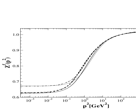
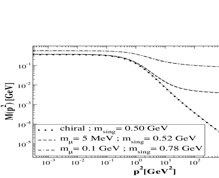
Figure 13: The functions $Z^{f}(p^{2})$ (left) and $M(p^{2})$ (right) obtained from parameterizations of $\sigma_{s,v}(p^{2})$, Eqs. (55)–(57), fitted to the numerical DSE solutions for different current quark masses. The solid curves are the fits, with the fit parameters given in Table 4.

Finally, we construct a parameterization of the inverse quark propagator functions $A(p^{2})$ and $B(p^{2})$, such that the propagator functions $\sigma_{s,v}(p^{2})$ have pole-like singularities on the timelike $p^{2}$ axis. For this purpose we use the parameterization

$$Z_{2}\;A(p^{2}) = 1+\frac{\alpha(p^{2}+m_{\hbox{\scriptsize sing}}^{2})}{2\pi}+\frac{C_{2}}{p^{2}+m_{\hbox{\scriptsize sing}}^{2}+\Lambda^{2}}\;,$$ (58)

$$Z_{2}\;B(p^{2}) = C_{dcsb}\;\frac{\alpha(p^{2}+m_{\hbox{\scriptsize sing}}^{2})^{1-\gamma_{m}}}{p^{2}+m_{\hbox{\scriptsize sing}}^{2}+\Lambda^{2}}+\frac{C_{4}}{(p^{2}+m_{\hbox{\scriptsize sing}}^{2}+\Lambda^{2})^{2}}+C_{cqm}\;\alpha(p^{2}+m_{\hbox{\scriptsize sing}}^{2})^{\gamma_{m}}\,,$$ (59)

with

$$m_{\hbox{\scriptsize sing}} = \left(C_{dcsb}\;\frac{\alpha(0)^{1-\gamma_{m}}}{\Lambda^{2}}+\frac{C_{4}}{\Lambda^{4}}+C_{cqm}\;\alpha(0)^{\gamma_{m}}\right)\bigg{/}\left(1+\frac{\alpha(0)}{2\pi}+\frac{C_{2}}{\Lambda^{2}}\right)\;,$$ (60)

and $Z_{2}$ determined by the renormalization condition $A(\mu^{2})=1$. The results of these fits are shown in Fig. 14, with the corresponding parameters given in Table 4. Though not as good as the direct fits of $Z^{f}(p^{2})$ and $M(p^{2})$ (Eqs. (51) and (52)) that were made without taking into consideration the analytic structure of $\sigma_{s,v}(p^{2})$, these fits reproduce the DSE results within about 10 to 20% over a wide range of masses. By construction, the dressing functions again reduce to the perturbative forms in the ultraviolet region and the analytic structure is in agreement with the Schwinger functions corresponding to our DSE solutions. In the chiral limit, $\Delta_{s}(t)$ corresponding to these fits shows significant curvature at small $t$, as can be seen from Fig. 12; for larger quark masses this curvature decreases. In contrast, $\Delta_{v}(t)$ does not show this curvature in agreement with our DSE results. However, the actual analytic structure of $\sigma_{s,v}(p^{2})$ is rather complicated. In addition to the singularity on the negative real axis at $p^{2}=-m_{\hbox{\scriptsize sing}}^{2}$ where a branch cut starts, it also has a pair of complex conjugate poles at zeros of $p^{2}\,A^{2}(p^{2})+B^{2}(p^{2})$.

     

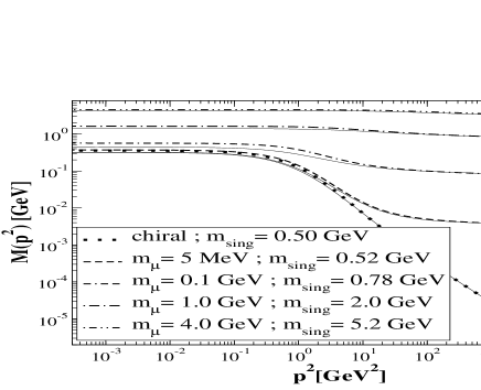
Figure 14: The functions $Z^{f}(p^{2})$ (left) and $M(p^{2})$ (right) obtained from parameterizations of $A(p^{2})$ and $B(p^{2})$, Eqs. (58)–(60), fitted to the numerical DSE solutions for different current quark masses. The solid curves are the fits, with the fit parameters given in Table 4.

IV.3 Generic features of the quark propagator

The results of this section point strongly towards an analytical structure of the quark propagator with a dominant singularity on the real timelike axis. At present, the nature of this singularity cannot be determined with confidence. It could be a simple pole, in which case additional poles or other types of singularities further away from $p^{2}=0$ are needed in order to explain the observed behavior of the Schwinger function. However, given the structure of the quark DSE, it is more likely that this singularity is a branch point, and that there is a branch cut along the negative real axis starting there. Having only one branch point singularity on the negative real axis is (in principle) sufficient to reproduce the observed Schwinger functions. We have not yet been able to distinguish between these alternatives by numerical calculations of the Schwinger functions of the DSE solutions.

Given the strong sensitivity of the Schwinger functions to the details of the propagator functions, and the fact that the dominant singularity is well into the timelike region, it is unlikely that the sub-dominant analytic structure of the quark propagator will be determined by Euclidean lattice simulations. The situation for the gluon propagator is quite different: there, the analytic structure is highly constrained by the behavior for $p^{2}\to 0^{+}$. By approaching the singularity at $p^{2}=0$ from the spacelike region, we can gain information about the nature of this singularity. In contrast, the first non-analytic point of the quark propagator is (most likely) at $p^{2}=-m_{\hbox{\scriptsize sing}}^{2}<0$. Thus, the behavior of $M(p^{2})$ and $Z^{f}(p^{2})$, or $\sigma_{s,v}(p^{2})$, for $p^{2}\to 0^{+}$ does not reveal much about the analytic properties of the propagator. We cannot approach the singularity without accessing the timelike region explicitly. In addition to this dominant singularity on (or very close to) the negative $p^{2}$ axis, the propagator may have other sub-leading singularities further away from $p^{2}=0$. Within the DSE framework one would have to solve the quark DSE over a suitable region of the complex momentum plane to decide questions about the nature of the dominant singularity and about the existence of sub-leading singularities further from $p^{2}=0$. However, this is numerically very demanding and not within the scope of the present investigation. As we have seen in the previous section, the results could also be strongly influenced by the truncation of the DSEs.

In all of the parameterizations of the preceding subsections a robust feature appears: the leading singularity is on (or very near to) the real axis. The scale at which this singularity occurs is somewhat dependent on the constraints used in the fits; the lattice data suggest a scale of 350 to 390 MeV, whilst the DSE solutions prefer a slightly larger value $\sim 500$ MeV. Despite this slight variation, these numerical values are somewhat intriguing and hint at a possible interpretation in terms of a constituent quark mass.

Fits like the examples presented here might be usefully applied in hadron phenomenology pending a more conclusive investigation of the analytic properties of the quark propagators. However, one should treat these parameterizations with care and keep in mind that neither the fitting forms nor the parameters are unique. The same Euclidean data, from lattice or DSE calculations, can be fitted quite well with different parameterizations having distinct analytic properties. The only robust feature concerning the analytic structure is that the dominant singularity, as probed by the Schwinger function, is on (or very near) the real timelike axis.

V Summary and Conclusion

In this work we have investigated the analytic structure of the propagators of Landau gauge QCD in the timelike momentum region using Schwinger functions, and employing various analytic parameterizations. We summarize the main results below.

Both lattice simulations and Dyson-Schwinger equation calculations suggest that the gluon propagator is finite or even vanishes in the infrared. The latter behavior necessarily leads to violations of reflection positivity, a sufficient (but not necessary) condition for gluon confinement. Our numerical analysis of the Schwinger functions calculated from the DSE solutions confirms this behavior, finding clear evidence of such positivity violations in the gluon propagator in accordance with previous results vonSmekal:1997is ; Langfeld:2002dd ; Fischer:2003rp . The gluon Schwinger function possesses one zero at $t\sim 1\;{\rm fm}$, marking the length scale above which sizable negative norm contributions appear. We explore the detailed analytic structure of the gluon propagator in the timelike ($p^{2}<0$) momentum region by constructing parameterizations that fit both the spacelike momentum behavior of the lattice calculations and DSE solutions, and the corresponding Schwinger function. These parameterizations incorporate the power-law infrared behavior determined analytically from the coupled ghost and gluon DSEs, and the perturbatively calculable ultraviolet logarithmic behavior. The crucial feature of these parameterizations is the presence of a branch cut on the timelike momentum half-axis which produces the observed positivity violations. These simple parameterizations depend on (effectively) only one parameter, the scale $\Lambda_{QCD}$.

In exploring the analytic structure of the quark propagator using the same Schwinger function methods, we have found an unexpected sensitivity of this structure to the truncation of the quark DSE. Gauge symmetry (or, more precisely, the relevant Slavnov–Taylor identity) requires the presence of a scalar coupling in the non-perturbative quark-gluon vertex. This coupling is only present if chiral symmetry is broken dynamically, in which case it leads to a self-consistent enhancement of the effective quark-gluon interaction. This term is important in at least two ways. First, it is required in order that the solution of the coupled quark, gluon, and ghost DSEs generates enough dynamical chiral symmetry breaking in the quark propagator to give a phenomenologically acceptable quark condensate Fischer:2003rp . More importantly for our investigations, the scalar coupling leads to qualitative changes in the analytic structure of the quark propagator, and hence has significant consequences for the questions of (non-)positivity and the manifestation of confinement. When this term is omitted (as in the commonly used rainbow truncation), positivity violations consistent with complex conjugate singularities in the quark propagator (as found in previous studies Bhagwat:2003vw ; Stainsby:1990fh ; Maris:1991cb ; Bender:1996bm ) are unambiguously observed. However, when the gauge-mandated scalar coupling is included, no such evidence of positivity violation is found and the dominant analytic structure appears to be a singularity on the real, timelike ($p^{2}<0$) axis. Whilst the absence of positivity violations says nothing about quark confinement (positivity violation is a sufficient but not necessary condition), it does tell us that confinement is probably not manifest at the level of the propagator. We also see similar behavior in (quenched) QED₄. Here, a positive definite propagator is desirable as the electron is an observable particle.

Finally in Sec. IV, we have attempted to probe deeper into the analytic structure of the quark propagator. We have constructed various parameterizations and used lattice data, DSE solutions, and other general properties to constrain them. Whilst an infinite variety of functional forms (we have investigated only a few that come easily to mind – constructed from real or complex conjugate poles, and branch cuts on the timelike momentum axis) would be capable of satisfying our constraint criteria, one robust feature emerges from our analysis: the dominant (i.e., closest to $p^{2}=0$) analytic structure occurs on (or very near to) the real, timelike half-axis. The scale of this mass-like singularity, as suggested by meromorphic parameterizations of the lattice data, is 350 to 390 MeV. The DSE solution indicates a scale of about 500 MeV. An accurate determination of the precise nature of this singularity and additional sub-dominant contributions awaits future improvements.

Appendix A Further details of the DSE truncation

Since the quark-gluon vertex appears to play a significant role in the analytic properties of the quark propagator, we have explicitly explored the effects of this part of our truncation scheme in the main body of the text. Here we examine the various truncations we use in the Yang-Mills sector and investigate reasonable modifications to highlight the extent of both the truncation dependence and the truncation independence of our results.

In this work, we have used the perturbative ghost-gluon vertex

$$\Gamma_{\mu}^{ghost}(q,p)=iq_{\mu}\,.$$ (61)

Lerche and von Smekal Lerche:2002ep have investigated a large class of possible structures for this Green’s function. In particular their results show that such variation leads to infrared behaviour of the gluon and ghost propagators as in Eqs. (18) and (19) with the exponent $\kappa$ in the range $0.5<\kappa<0.7$. In this range the essential analytic properties that we find for the gluon propagator remain unaltered.

For the three-gluon vertex, we use Fischer:2003zc

$$\Gamma_{\rho\nu\sigma}(q,p)=\frac{1}{Z_{1}(\mu,\Lambda)}\frac{G(q^{2})^{(1-a/\delta-2a)}}{Z(q^{2})^{(1+a)}}\frac{G((q-p)^{2})^{(1-b/\delta-2b)}}{Z((q-p)^{2})^{(1+b)}}\Gamma^{(0)}_{\rho\nu\sigma}(q,p)$$ (62)

where $\Gamma^{(0)}_{\rho\nu\sigma}(q,p)$ is the perturbative form, $\delta=-9N_{c}/(44N_{c}-8N_{f})$ is the one-loop anomalous dimension of the ghost propagator, $Z_{1}$ is the three-gluon vertex renormalisation, and we fix $a=b=3\delta$. As discussed in the main text, this form is chosen to ensure the running coupling, Eq. (16), is renormalisation point independent and that the ghost and gluon propagators have the correct one-loop anomalous dimensions (these constraints are satisfied for arbitrary values of the parameters $a$ and $b$).

Whilst no systematic study of this vertex truncation exists, in Ref. Fischer:2003zc one of us has investigated some variation of the parameters $a$ and $b$. There, the gluon propagator was found to vanish at $p^{2}\to 0$ independent of the choice of $a$ and $b$, and our conclusions about the analytic structure of the gluon propagator remain qualitatively unchanged. To investigate the dependence of the gluon fit parameters ($\omega_{I,II}$ and $\Lambda_{QCD}$) on the three-gluon vertex truncation, we have made fits to the quenched DSE solutions using Eq.(33) for a number of choices of $a$ and $b$. The resulting parameter sets are shown in Table 5 and are seen to vary by 20%. With certain choices of these parameters, one is able to closely match the quenched lattice data. However the original ($a=b=3\delta$) truncation gives results in adequate agreement (see Fig. 2) with this data (which itself is not without error bars) and we use it exclusively in the main text.

Truncation	Fit I		Fit II
	$\omega_{I}$	$\Lambda_{QCD}$ [MeV]	$\omega_{II}$	$\Lambda_{QCD}$ [MeV]
Full QCD, $a=3\delta$	2.4(2.0)	500(470)	2.5	510
Quenched QCD, $a=3\delta$	2.9	550	3.2	550
Quenched QCD, $a=2\delta$	2.7	410	3.0	400
Quenched QCD, $a=4\delta$	3.2	560	3.6	550

Table 5: Gluon fit parameters for various truncations of the system of DSEs. The parenthesized results for the full QCD fit I are when the fit is optimized to reproduce fit the DSE Schwinger function; all other parameter sets are fitted to $Z(p)$.

Finally, the truncation we employ neglects the effects of the four-gluon vertex. These effects are unknown up to now. Since the ghost loop is dominant in the infrared Zwanziger:2003cf and the one-loop diagrams dominate in the perturbative, ultraviolet region, such effects are expected to be most important in the intermediate momentum regime ($p^{2}\sim 1$GeV²). A two-parameter model for the corresponding two-loop diagrams in the coupled gluon-ghost DSEs has been explored in Ref. Bloch:2003yu ; under such variation the $p^{2}\to 0$ behaviour of the gluon and ghost propagator remains qualitatively the same as in our results.

Appendix B Pole or branch point in the quark propagator?

If the quark propagator has a non-analytic point at $p^{2}=-m_{\hbox{\scriptsize sing}}^{2}$ where the propagator diverges, what kind of singularity can we expect? In order to answer this question, consider the generic integral that appears in the RHS of the quark DSE

$$I(p^{2})\;=\;\int^{\Lambda}d^{4}q\,\frac{\alpha((q-p)^{2})}{(q-p)^{2}}\;K_{\theta}(q^{2},p^{2},q\cdot p)\;\sigma_{s,v}(q^{2})\;.$$ (63)

Assume that the running coupling, $\alpha(k^{2})$, does not go to zero like $k^{2}$ for $k^{2}\to 0$. Furthermore, assume that the kernel $K_{\theta}(q^{2},p^{2},q\cdot p)$ has no singularities. Thus the only singularities in the integrand are located at $(q-p)^{2}=0$ and at $q^{2}=-m_{\hbox{\scriptsize sing}}^{2}$ (coming from the propagator function $\sigma_{s,v}(q^{2})$). For Euclidean values of $p^{2}$, we calculate this integral by performing the angular integral first, followed by the radial integral

$$I(p^{2})\;=\;\int_{0}^{\Lambda^{2}}q^{2}dq^{2}\,\sigma_{s,v}(q^{2})\;K(q^{2},p^{2})\;,$$ (64)

with

$$K(q^{2},p^{2})\;=\;\int_{0}^{\pi}\sin^{2}\theta\;d\theta\frac{\alpha(q^{2}-2qp\cos\theta+p^{2})}{q^{2}-2qp\cos\theta+p^{2}}\;K_{\theta}(q^{2},p^{2},qp\cos\theta)\;.$$ (65)

This angular integral is well-behaved for any Euclidean value of $q^{2}$ and $p^{2}$ as long as the singularity in $\alpha(k^{2})/k^{2}$ is an integrable singularity, so let us assume from here on that this is the case. If we investigate the analytic properties of $K(q^{2},p^{2})$ for arbitrary complex values of $q^{2}$, while keeping $p^{2}$ real and positive, we discover that it has a branch cut that can be characterized by $q^{2}=p^{2}\exp(i\phi)$, with $0<\phi<2\pi$. Notice that if we perform the radial integral along the positive real $q^{2}$ axis, we do not cross this branch cut: the end-points in $\phi$ are not included. This is schematically depicted in Fig. 15.

Figure 15: Location of the branch cuts (dotted curves) in $K(q^{2},p^{2})$ in the complex $q^{2}$-plane, for $p^{2}=x$ being real and for a complex value of $p^{2}=x+i\,y$. Also shown are possible integration paths (solid curves) from $0$ to $\Lambda^{2}$ that do not cross the corresponding branch cuts.

Now consider the analytic continuation to complex values of $p^{2}$. Clearly, the branch cut in $K(q^{2},p^{2})$ will move, as indicated in Fig. 15. This means that the integration path in Eq. (64) has to be deformed so as not to cross the (shifted) branch cut stemming from the angular integration, while keeping the end-points fixed. A possible integration path has been shown in Fig. 15, though the actual integration path is of course not unique. The general rule for this deformed integration path is that it has to go through the point $q^{2}=p^{2}$, since that is where there is an opening in the circular branch cut of $K(q^{2},p^{2})$. This procedure leads to a well-defined and unambiguous analytic continuation of the Euclidean DSE, and can be implemented numerically Maris:1995ns ; pmthesis .

Figure 16: Two integration contours in the complex $k^{2}$-plane for the radial integral in $I(p^{2})$ for $p^{2}=x-iy$ (left) and the resulting analytic structure for $I(p^{2})$ in the complex $p^{2}$-plane (right).

Following this procedure, one can now show that any singularity in $\sigma_{s,v}(q^{2})$ leads (in general) to a branch point singularity in $I(p^{2})$. This is shown in detail in Fig. 16 for the case in which $\sigma_{s,v}(q^{2})$ have singularities on the real time-like axis at $q^{2}=-m_{\hbox{\scriptsize sing}}^{2}$. We have drawn two distinct radial integration paths in order to calculate $I(p^{2})$ for $p^{2}=x-iy$. One is obtained by continuously deforming the original integration path through the upper half of the complex $q^{2}$-plane, crossing the negative real axis beyond $q^{2}=-m_{\hbox{\scriptsize sing}}^{2}$ (dashed curve), and the other by deforming the integration path via the lower half of the complex plane (solid curve). Because of the combination of (i) the singularity in $\sigma_{s,v}(q^{2})$ at $q^{2}=-m_{\hbox{\scriptsize sing}}^{2}$ and (ii) the circular branch cut in $K(q^{2},p^{2})$, these two integration paths cannot be deformed into each other while keeping $p^{2}$ fixed. Therefore, the obtained values of $I(p^{2})$ will (in general) be different, and $I(p^{2})$ becomes a multi-valued function with a branch-point singularity at $p^{2}=-m_{\hbox{\scriptsize sing}}^{2}$. The “natural” choice for the branch cut is along the negative real axis, as indicated by the wavy line in the right panel of Fig. 16.

Returning to the specific case of the quark propagator, we note that the RHS of the quark DSE contains an integral like $I(p^{2})$, whereas the LHS is one of the inverse quark propagator functions $A(p^{2})$ or $B(p^{2})$. If $\sigma_{v,s}(q^{2})$ has a singular point $k^{2}=-m_{\hbox{\scriptsize sing}}^{2}$, then $I(p^{2})$ has a branch-point singularity at $p^{2}=-m_{\hbox{\scriptsize sing}}^{2}$, and therefore $A(p^{2})$ and $B(p^{2})$ will have a branch point at $p^{2}=-m_{\hbox{\scriptsize sing}}^{2}$. Thus, unless there are intricate cancellations, the singularity in $\sigma_{v,s}(p^{2})$ of a self-consistent solution is a branch-point singularity and not a simple pole.

References

- (1)
- (2) I. Montvay and G. Munster, “Quantum Fields On A Lattice,” Cambridge Univ. Press (1994), Cambridge, UK.
- (3) H. J. Rothe, “Lattice Gauge Theories: An Introduction”, World Sci. Lect. Notes Phys. 59, 1 (1997).
- (4) R. Alkofer and L. von Smekal, Phys. Rept. 353, 281 (2001) [arXiv:hep-ph/0007355].
- (5) C. D. Roberts and S. M. Schmidt, Prog. Part. Nucl. Phys. 45, S1 (2000) [arXiv:nucl-th/0005064].
- (6) P. Maris and C. D. Roberts, Int. J. Mod. Phys. E 12, 297 (2003) [arXiv:nucl-th/0301049].
- (7) L. von Smekal, R. Alkofer and A. Hauck, Phys. Rev. Lett. 79, 3591 (1997) [arXiv:hep-ph/9705242]; L. von Smekal, A. Hauck and R. Alkofer, Annals Phys. 267, 1 (1998) [arXiv:hep-ph/9707327]; A. Hauck, L. von Smekal and R. Alkofer, Comput. Phys. Commun. 112 (1998) 166 [arXiv:hep-ph/9804376].
- (8) D. Atkinson and J. C. Bloch, Mod. Phys. Lett. A 13, 1055 (1998) [arXiv:hep-ph/9802239]. Phys. Rev. D 58 (1998) 094036 [arXiv:hep-ph/9712459].
- (9) C. Lerche and L. von Smekal, Phys. Rev. D 65, 125006 (2002) [arXiv:hep-ph/0202194].
- (10) D. Zwanziger, Phys. Rev. D 65, 094039 (2002) [arXiv:hep-th/0109224].
- (11) C. S. Fischer and R. Alkofer, Phys. Lett. B536, 177 (2002) [arXiv:hep-ph/0202202]; C. S. Fischer, R. Alkofer and H. Reinhardt, Phys. Rev. D65, 094008 2002 [arXiv:hep-ph/0202195]; R. Alkofer, C. S. Fischer and L. von Smekal, Acta Phys. Slov. 52, 191 (2002) [arXiv:hep-ph/0205125]; C. S. Fischer, PhD thesis, U. of Tuebingen, arXiv:hep-ph/0304233.
- (12) C. S. Fischer and R. Alkofer, Phys. Rev. D 67, 094020 (2003) [arXiv:hep-ph/0301094].
- (13) P. C. Tandy, Prog. Part. Nucl. Phys. 50, 305 (2003) [arXiv:nucl-th/0301040].
- (14) M. S. Bhagwat et al., Phys. Rev. C 68, 015203 (2003) [arXiv:nucl-th/0304003].
- (15) T. Kugo and I. Ojima, Prog. Theor. Phys. Suppl. 66 (1979) 1.
- (16) N. Nakanishi and I. Ojima, “Covariant Operator Formalism Of Gauge Theories And Quantum Gravity,” World Sci. Lect. Notes Phys. 27, 1 (1990).
- (17) T. Kugo, Int. Symp. on BRS symmetry, Kyoto, Sep. 18-22, 1995, arXiv:hep-th/9511033.
- (18) F. Strocchi, Phys. Rev. D 17, 2010 (1978).
- (19) P. van Baal, arXiv:hep-th/9711070.
- (20) J. Greensite, arXiv:hep-lat/0301023.
- (21) H. Suman and K. Schilling, Phys. Lett. B373 (1996) 314–318, [arXiv:hep-lat/9512003].
- (22) K. Langfeld et al., arXiv:hep-th/0209173.
- (23) S. Furui and H. Nakajima, arXiv:hep-lat/0305010.
- (24) K. Osterwalder and R. Schrader, Commun. Math. Phys. 31 (1973) 83–112; Commun. Math. Phys. 42 (1975) 281.
- (25) R. Haag, “Local quantum physics: Fields, particles, algebras,” Berlin, Germany: Springer (1992) 356 p. (Texts and monographs in physics).
- (26) J. Glimm and A. Jaffe, “Quantum Physics. A Functional Integral Point Of View,” 2nd ed. (Springer, NY 1987)
- (27) R. Oehme, Int. J. Mod. Phys. A 10, 1995 (1995) [arXiv:hep-th/9412040].
- (28) L. C. Hollenberg, C. D. Roberts and B. H. McKellar, Phys. Rev. C 46 (1992) 2057; M. Burkardt, M. R. Frank and K. L. Mitchell, Phys. Rev. Lett. 78, 3059 (1997) [arXiv:hep-ph/9611256].
- (29) U. Habel et al., Z. Phys. A 336 (1990) 423; Z. Phys. A 336 (1990) 435; M. Stingl, Z. Phys. A353 (1996) 423–445, [arXiv:hep-th/9502157].
- (30) P. Maris, Phys. Rev. D 52 (1995) 6087 [arXiv:hep-ph/9508323].
- (31) D. Atkinson and D. W. Blatt, Nucl. Phys. B 151 (1979) 342.
- (32) S. J. Stainsby and R. T. Cahill, Phys. Lett. A 146, 467 (1990); Int. J. Mod. Phys. A 7, 7541 (1992).
- (33) P. Maris and H. A. Holties, Int. J. Mod. Phys. A 7, 5369 (1992).
- (34) A. Bender et al., Phys. Rev. Lett. 77 (1996) 3724 [arXiv:nucl-th/9606006].
- (35) A. Bender et al., Phys. Lett. B 431 (1998) 263 [arXiv:nucl-th/9710069].
- (36) C. J. Burden, Phys. Rev. D 57, 276 (1998) [arXiv:hep-ph/9702411]; Phys. Rev. D 59, 037502 (1999) [arXiv:hep-ph/9807438].
- (37) G. Krein, C. D. Roberts and A. G. Williams, Int. J. Mod. Phys. A 7, 5607 (1992).
- (38) C. J. Burden, C. D. Roberts and A. G. Williams, Phys. Lett. B 285, 347 (1992).
- (39) B. C. Tiburzi, W. Detmold and G. A. Miller, Phys. Rev. D 68, 073002 (2003) [arXiv:hep-ph/0305190].
- (40) M. S. Bhagwat, M. A. Pichowsky and P. C. Tandy, Phys. Rev. D 67, 054019 (2003).
- (41) V. N. Gribov, Nucl. Phys. B139 (1978) 1.
- (42) D. Zwanziger, Nucl. Phys. B 378, 525 (1992).
- (43) L. Driesen et al., Eur. Phys. J. A 4, 381 (1999) [arXiv:hep-th/9808152]; L. Driesen and M. Stingl, Eur. Phys. J. A 4, 401 (1999) [arXiv:hep-th/9808155].
- (44) F. T. Hawes, C. D. Roberts and A. G. Williams, Phys. Rev. D 49 (1994) 4683 [arXiv:hep-ph/9309263].
- (45) A. Bender and R. Alkofer, Phys. Rev. D 53 (1996) 446 [arXiv:hep-ph/9411266].
- (46) J. M. Jauch and F. Rohrlich, “The Theory of Photons and Electrons,” Springer Verlag, 2nd edition, 1976.
- (47) D. Zwanziger, Phys. Rev. D 69, 016002 (2004) [arXiv:hep-ph/0303028].
- (48) P. Watson and R. Alkofer, Phys. Rev. Lett. 86, 5239 (2001) [arXiv:hep-ph/0102332];
- (49) R. Alkofer, L. von Smekal and P. Watson, arXiv:hep-ph/0105142.
- (50) L. D. Faddeev and V. N. Popov, Phys. Lett. B 25, 29 (1967).
- (51) J. C. Taylor, Nucl. Phys. B 33, 436 (1971); J. C. R. Bloch, A. Cucchieri, K. Langfeld and T. Mendes, arXiv:hep-lat/0312036.
- (52) J. C. R. Bloch, Few Body Syst. 33, 111 (2003) [arXiv:hep-ph/0303125].
- (53) J. M. Pawlowski, D. F. Litim, S. Nedelko and L. von Smekal, arXiv:hep-th/0312324; C. S. Fischer and H. Gies, in preparation.
- (54) C. D. Roberts and A. G. Williams, Prog. Part. Nucl. Phys. 33 (1994) 477 [arXiv:hep-ph/9403224].
- (55) W. Detmold, Phys. Rev. D 67, 085011 (2003) [arXiv:hep-ph/0301007].
- (56) D. C. Curtis and M. R. Pennington, Phys. Rev. D 42, 4165 (1990).
- (57) J. S. Ball and T. W. Chiu, Phys. Rev. D 22 (1980) 2542.
- (58) A. Bender et al., Phys. Rev. C 65, 065203 (2002) [arXiv:nucl-th/0202082].
- (59) A. Bender, C. D. Roberts and L. von Smekal, Phys. Lett. B 380, 7 (1996) [arXiv:nucl-th/9602012].
- (60) G. Hellstern, R. Alkofer and H. Reinhardt, Nucl. Phys. A 625, 697 (1997) [arXiv:hep-ph/9706551].
- (61) P. Maris and C. D. Roberts, Phys. Rev. C 56 (1997) 3369 [arXiv:nucl-th/9708029].
- (62) P. Maris and P. C. Tandy, Phys. Rev. C 60 (1999) 055214 [arXiv:nucl-th/9905056].
- (63) R. Alkofer, P. Watson and H. Weigel, Phys. Rev. D 65 (2002) 094026 [arXiv:hep-ph/0202053]; H. Weigel, R. Alkofer and P. Watson, arXiv:hep-ph/0307066,
- (64) F. D. Bonnet et al., Phys. Rev. D 64, 034501 (2001) [arXiv:hep-lat/0101013];
- (65) D. Zwanziger, Nucl. Phys. B 323 (1989) 513.
- (66) D. V. Shirkov and I. L. Solovtsov, Phys. Rev. Lett. 79 (1997) 1209 [arXiv:hep-ph/9704333].
- (67) N. K. Nielsen, Nucl. Phys. B 101 (1975) 173.
- (68) J. E. Mandula and M. Ogilvie, Phys. Lett. B 185 (1987) 127;
- (69) P. Marenzoni et al., Phys. Lett. B 318 (1993) 511; C. W. Bernard, C. Parrinello and A. Soni, Phys. Rev. D 49, 1585 (1994) [arXiv:hep-lat/9307001]; A. Nakamura et al., arXiv:hep-lat/9506024; H. Nakajima and S. Furui, Nucl. Phys. Proc. Suppl. 73, 635 (1999) [arXiv:hep-lat/9809081]; D. Becirevic et al., Phys. Rev. D 61, 114508 (2000) [arXiv:hep-ph/9910204]; C. Alexandrou, P. de Forcrand and E. Follana, Phys. Rev. D 63, 094504 (2001) [arXiv:hep-lat/0008012]; A. Cucchieri and D. Zwanziger, Phys. Rev. D 65, 014001 (2002) [arXiv:hep-lat/0008026]; D. B. Leinweber et al., Phys. Rev. D 58 (1998) 031501 [arXiv:hep-lat/9803015]. F. D. Bonnet et al., Phys. Rev. D 62, 051501 (2000) [arXiv:hep-lat/0002020]; P. O. Bowman et al., Phys. Rev. D 66, 074505 (2002) [arXiv:hep-lat/0206010]; K. Langfeld, H. Reinhardt and J. Gattnar, Nucl. Phys. B 621, 131 (2002) [arXiv:hep-ph/0107141]; V. G. Bornyakov et al., arXiv:hep-lat/0308028.
- (70) J. E. Mandula, Phys. Rept. 315 (1999) 273.
- (71) K. Langfeld, H. Reinhardt and J. Gattnar, Nucl. Phys. B 621, 131 (2002) [arXiv:hep-ph/0107141].
- (72) A. Cucchieri, private correspondence and A. Cucchieri, T. Mendes and A. R. Taurines, Phys. Rev. D 67, 091502 (2003) [arXiv:hep-lat/0302022];
- (73) F. D. Bonnet et al., Phys. Rev. D 65, 114503 (2002) [arXiv:hep-lat/0202003]. J. B. Zhang et al., arXiv:hep-lat/0208037. J. B. Zhang et al., arXiv:hep-lat/0301018.
- (74) P. O. Bowman, U. M. Heller and A. G. Williams, Phys. Rev. D 66, 014505 (2002) [arXiv:hep-lat/0203001].
- (75) D. Jarecke, P. Maris and P. C. Tandy, Phys. Rev. C 67 (2003) 035202 [arXiv:nucl-th/0208019].
- (76) J. C. Bloch, Phys. Rev. D 66 (2002) 034032 [arXiv:hep-ph/0202073].
- (77) J. I. Skullerud et al., JHEP 0304, 047 (2003) [arXiv:hep-ph/0303176].
- (78) R. Oehme and W. T. Xu, Phys. Lett. B 384, 269 (1996) [arXiv:hep-th/9604021].
- (79) K. D. Lane, Phys. Rev. D 10, 2605 (1974); H. D. Politzer, Nucl. Phys. B 117, 397 (1976).
- (80) J. I. Skullerud and A. G. Williams, Phys. Rev. D 63, 054508 (2001) [arXiv:hep-lat/0007028]. J. Skullerud, D. B. Leinweber and A. G. Williams, Phys. Rev. D 64, 074508 (2001) [arXiv:hep-lat/0102013].
- (81) P. O. Bowman et al., arXiv:hep-lat/0209129.
- (82) C. D. Roberts, arXiv:nucl-th/0007054.
- (83) F. Karsch et al., Nucl. Phys. Proc. Suppl. 73, 213 (1999) [arXiv:hep-lat/9809011].
- (84) C. S. Fischer, “Non-perturbative propagators, running coupling and dynamical mass generation in ghost - antighost symmetric gauges in QCD,” PhD thesis, University of Tuebingen, arXiv:hep-ph/0304233.
- (85) P. Maris, “Nonperturbative analysis of the fermion propagator: complex singularities and dynamical mass generation”, PhD thesis, University of Groningen, 1993.