Using and Constraining Nonforward Parton Distributions
Deeply Virtual Neutrino Scattering in Cosmic Rays
and Light Dark Matter Searches

Claudio Corianò, G. Chirilli and Marco Guzzi

Dipartimento di Fisica, Università di Lecce
and INFN Sezione di Lecce
Via Arnesano 73100 Lecce, Italy

We overview the construction of Nonforward Parton Distributions (NPD) in Deeply Virtual Compton Scattering (DVCS). Then we turn to the analysis of similar constructs in the weak sector (electroweak NPD’s). We argue in favour of a possible use of electroweak DVCS (EWDVCS) as a rare process for the study of neutrinos in cosmic rays and for light dark matter detection in underground experiments.

1 Introduction

Nonforward Parton Distributions are an important construct in the parton model [1], [2] and appear in Compton Scattering (CS) (Fig. 1) in the generalized Bjorken region [3], where the process is hand-bag dominated. They generalize ordinary parton distributions (Fig. 2). Proofs of factorization to all orders of processes of this type have also been presented [4] and there is a large amount of work (see for instance [5]) devoted to the subject, accompanied by ongoing experimental efforts to measure the corresponding cross section [6]. In the electromagnetic case the measurements are difficult, given the presence of a dominant Bethe-Heitler background. One of the possibilities to perform the measurement is through the interference between the Bethe-Heitler and the DVCS hand-bag diagram by electron spin asymmetries.

The analysis of these distributions, including their modeling [17][18] and the theoretical and phenomenological study of the leading-twist and higher-twist contributions in the context of ordinary DVCS (with a virtual or a real final state photon) [10] has also progressed steadily. In this talk we will briefly outline some of the features of these distributions and elaborate on the possibility to use some variants of them in the description of electroweak processes induced by neutral and charged currents on nucleons. Possible applications of these generalizations which we are suggesting are in deeply virtual neutrino scattering for diffuse neutrinos and in the detection of light dark matter. Results of this analysis will be presented elsewhere.

2 The DVCS Domain

A pictorial description of the process we are going to illustrate is given in Fig. 3 where a lepton of momentum $l$ scatters off a nucleon of momentum $P_{1}\equiv p$ via a gauge boson exchange; from the final state a photon and a nucleon emerge, of momenta $q_{2}$ and $P_{2}\equiv=P^{\prime}=p+r$ respectively. In the deeply virtual limit, analogous to the usual Bjorken limit, the final state photon is on shell, and a large longitudinal (light cone) momentum exchanged is needed in order to guarantee factorization.

The regime for the study of NFPD’s is characterized by a deep virtuality of the exchanged photon in the initial interaction ($e+p\to e+p+\gamma$) ( $Q^{2}>$ 2 GeV²), with the final state photon kept on-shell, large energy of the hadronic system ($W^{2}>6$ GeV²) above the resonance region and small momentum transfers $|t|<1$ GeV². In the region of interest (large $Q^{2}$ and small $t$) the Bethe-Heitler background $(\sim 1/t)$ is dominant and the $1/Q$ behaviour of the virtual Compton scattering amplitude (VCS) render the analysis quite complex. A dedicated study of the interference BH-VCS in order to explore the generalized Bjorken region is therefore required.

2.1 Nonforward Parton Distributions

In the case of nonforward distributions a second scaling parameter $\zeta$ ($\xi$) controls the asymmetry between the initial and the final nucleon momentum in the deeply virtual limit of nucleon Compton scattering. Both the inclusive DIS region and the exclusive ERBL region can be analized with the same correlator. We recall that in the light-cone gauge the (off forward) distributions $H(x,\xi)$ [1] is defined as

$$H_{q}(x,\xi,\Delta^{2}))=\frac{1}{2}\int\frac{dy^{-}}{2\pi}e^{-ix\bar{P}^{+}y^{-}}\langle P^{\prime}|\bar{\psi}_{q}(0,\frac{y^{-}}{2},{\bf 0_{\perp}})\frac{1}{2}\gamma^{+}\psi_{q}(0,\frac{y^{-}}{2},{\bf 0_{\perp}})|P\rangle$$ (1)

with $\Delta=P^{\prime}-P$,$\Delta^{2}\equiv t$ $\bar{P}^{+}=1/2(P+\bar{P})$ [1] (symmetric choice) and $\xi\bar{P}=1/2\,\,\Delta^{+}$.

This distribution describes for $x>\xi$ and $x<-\xi$ the DGLAP-type region for the quark and the antiquark distribution respectively, and the ERBL (see [5], [14]) distribution amplitude for $-\xi<x<\xi$. In the following we will omit the $\Delta$ dependence from $H_{q}$.

The most common procedure is to use double distributions, $F(x,y)$ defined with a symmetric choice of the external momenta and relate them to off-forward distributions $H(v,\xi,t)$ [1], incorporating in a single interval with $-1\leq v\leq 1$ both the quark and antiquark parton distributions with an asymmetry parameter $\xi$,

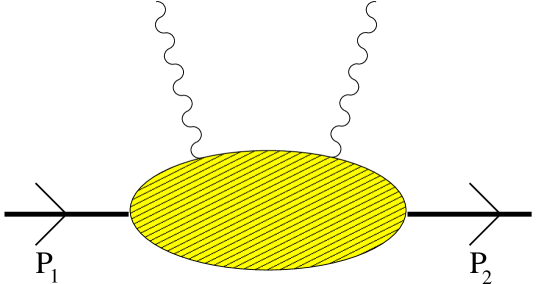
Figure 1: Compton Scattering

$$H(v,\xi,t)=$$

$$\int^{1}_{-1}dx^{\prime}\int^{1-|x^{\prime}|}_{-1+|x^{\prime}|}dy^{\prime}\delta(x^{\prime}+\xi y^{\prime}-v)F(x^{\prime},y^{\prime},t)\,,$$ (2)

Below we will neglect the $t$ dependence. The singlet/ nonsinglet decomposition of the evolution can be carried out as usual taking linear combination of flavours

$$H^{S}(v,\xi)=\sum_{a}H^{q,a}(v,\xi)\mp H^{q,a}(-v,\xi)\,,$$

$$H^{NS,a}(v,\xi)=H^{q,a}(v,\xi)\pm H^{q,a}(-v,\xi)\,,$$

$$H^{G}(v,\xi)=H^{g}(v,\xi)\pm H^{g}(-v,\xi).$$ (3)

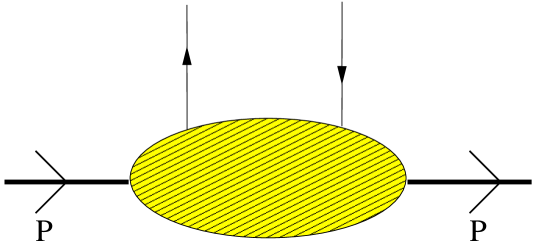
Figure 2: Forward Parton Distributions

The evolution can be analized in various ways. One possibility is to use nondiagonal distributions [11], related to the asymmetric distributions introduced by Radyushkin (see [5])

$${\cal F}^{q,a}\left(X_{1}=\frac{v_{1}+\xi}{1+\xi},\zeta\right)=\frac{H^{q,a}(v_{1},\xi)}{(1-\zeta/2)}\,,$$ (4)

$${\cal F}^{{\bar{q}},a}\left(X_{2}=\frac{\xi-v_{2}}{1+\xi},\zeta\right)=-\frac{H^{q,a}(v_{2},\xi)}{(1-\zeta/2)}\,,$$ (5)

where $v_{1}\in[-\xi,1],\,v_{2}\in[-1,\xi]$. The parameter $\zeta\equiv r_{+}/p_{+}$ characterizes the so-called $skewedness$ of the process and is defined in the interval $\zeta\in[0,1]$. Variables $\xi$ and $\zeta$ are related in the DVCS limit by $\xi=\zeta/(2-\zeta)$ and $\zeta=x_{bj}$, conciding with Bjorken variable x (modulo terms of ${\cal O}(x_{bj}t/Q^{2})$).

The inverse transformations between the $v$s and $X$s are easily found in the various allowed regions

$$v_{1}=\frac{X_{1}-\zeta/2}{1-\zeta/2} \,,\, v_{2}=\frac{\zeta/2-X_{2}}{1-\zeta/2}\,.$$ (6)

$${\cal F}^{g}(X,\zeta) = \frac{H^{g}(v,\xi)}{(1-\zeta/2)}\,.$$ (7)

In the gluon case one can use any either $v_{1}$ or $v_{2}$ equivalently.

One finds

$${\cal F}^{q,a}(X,\zeta)=\frac{H^{q,a}(v_{1},\xi)}{1-\zeta/2}=\int^{1}_{-1}dx^{\prime}\int^{1-|x^{\prime}|}_{-1+|x^{\prime}|}dy^{\prime}\delta\left(x^{\prime}+\xi y^{\prime}-v_{1}\right)\frac{F^{q,a}(x^{\prime},y^{\prime})}{\left(1-\zeta/2\right)}\,,$$

$${\cal F}^{{\bar{q}},a}(X,\zeta)=-\frac{H^{q,a}(v_{2},\xi)}{1-\zeta/2}=\int^{1}_{-1}dx^{\prime}\int^{1-|x^{\prime}|}_{-1+|x^{\prime}|}dy^{\prime}\delta\left(x^{\prime}+\xi y^{\prime}-v_{2}\right)\frac{F^{q,a}(x^{\prime},y^{\prime})}{\left(1-\zeta/2\right)}\,.$$ (8)

with $1>v_{1}>-\xi$, $-1<v_{2}<\xi$. The generation of initial conditions for nonforward distributions is usually based on factorization, as suggested originally by Radyushkin, starting from the double distributions ($x^{\prime}-y^{\prime}$ factorization). These are obtained using some profile functions $\pi()$ which characterizes the spreading in $y^{\prime}$ of the momentum transfer $r$, combined with an ordinary forward parton distributions. The latter is appropriately extended to the $x^{\prime}<0$ to describe antiquark components, as pointed out long ago [12]. For instance, in the quark/gluon case one obtains [18] [2]

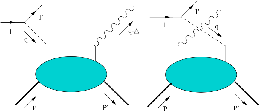
Figure 3: Leading hand-bag diagrams for the process

$$F^{q,a}(x^{\prime},y^{\prime}) = \pi^{q}(x^{\prime},y^{\prime})f^{q,a}(x^{\prime})$$

$$= \frac{3}{4}\frac{(1-|x^{\prime}|)^{2}-{y^{\prime}}^{2}}{(1-|x^{\prime}|)^{3}}f^{q,a}(x^{\prime})\,,$$

$$F^{g}(x^{\prime},y^{\prime}) = \pi^{g}(x^{\prime},y^{\prime})f^{g}(x^{\prime})$$ (9)

$$= \frac{15}{16}\frac{((1-|x^{\prime}|)^{2}-{y^{\prime}}^{2})^{2}}{(1-|x^{\prime}|)^{5}}f^{g}(x^{\prime})\,,$$

for quark of flavour $a$, where the quarks and gluon distributions are extended to $x<0$, as

$$f^{g}(x) = xg(x,Q_{0})\Theta(x)+|x|g(|x|,Q_{0})\Theta(-x)\,,$$

$$f^{q,a}(x) = q^{a}(x,Q_{0})\Theta(x)-(\bar{q}^{a})(|x|,Q_{0})\Theta(-x)\,.$$ (10)

$${\cal F}^{q,a}(X,\zeta)=\frac{2}{\zeta}\int^{\frac{v_{1}+\xi}{1+\xi}}_{\frac{v_{1}-\xi}{1-\xi}}dx^{\prime}\pi^{q}\left(x^{\prime},\frac{v_{1}-x^{\prime}}{\xi}\right)q^{a}(x^{\prime})\,.$$ (11)

For the anti-quark, since $v_{2}=-v_{1}$ one may use eqs.(5,8) with $v_{2}\to-v_{1}$, and, exploiting the fact that $f^{q}(x)=-{\bar{q}}(|x|)$ for $x<0$, one arrives at

$${\cal F}^{\bar{q},a}(X,\zeta)=\frac{2}{\zeta}\int^{\frac{-v_{1}+\xi}{1-\xi}}_{\frac{-v_{1}-\xi}{1+\xi}}dx^{\prime}\pi^{q}\left(x^{\prime},\frac{-v_{1}-x^{\prime}}{\xi}\right){\bar{q}}^{a}(|x^{\prime}|).$$ (12)

The expression for the gluons is similar. Performing the y’ integration, one obtains in the two regions, DGLAP and ERBL respectively

$${\cal F}^{g}(X,\zeta)=\frac{2}{\zeta}\int_{\frac{X-\zeta}{1-\zeta}}^{X}dx^{\prime}\pi^{g}\left(x^{\prime},{\tilde{y}}(x^{\prime})\right)\leavevmode\nobreak\ x^{\prime}g(x^{\prime})\,,$$ (13)

and

$${\cal F}^{g}(X,\zeta) =\frac{2}{\zeta}\Big{[}\int_{0}^{X}dx^{\prime}\pi^{g}\left(x^{\prime},{\tilde{y}}(x^{\prime})\right)\leavevmode\nobreak\ x^{\prime}g(x^{\prime})$$ (14)

$$+\int_{0}^{\zeta-X}dx^{\prime}\pi^{g}\left(x^{\prime},{\tilde{y}}(-x^{\prime})\right)\leavevmode\nobreak\ x^{\prime}g(x^{\prime})\Big{]}.$$

2.2 A Comment

Parton distributions are quasi-probabilities, very similar to Wigner functions (as first observed in [7]), though the momentum dependence of the latter is not found easily found in the former. One possibility in this direction has been suggested recently [8]. The formal definition of a parton distributions is in a non-local light cone correlator, built through unitarity (at least in the forward case). In the nonforward case there is no optical theorem (Fig. 4) that holds, and the construct is a genuine correlation function in the nucleon state. We have pointed out in [7] the existence of a formal relation between evolution equations and kinetic equations, via a Kramers-Moyal expansion of the non-forward evolution equation. This relation carries a strong similarity to the well known relation between Wigner functions and their associated evolution equations, given by differential operators of arbitrarily high orders (Moyal products) as known from the phase-space approach to quantum mechanics [9]. Indeed the definition of a parton distribution takes place through a Wigner-Weyl transform, limited to the light cone domain.

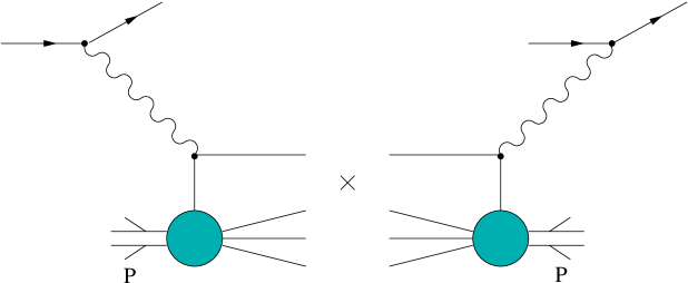
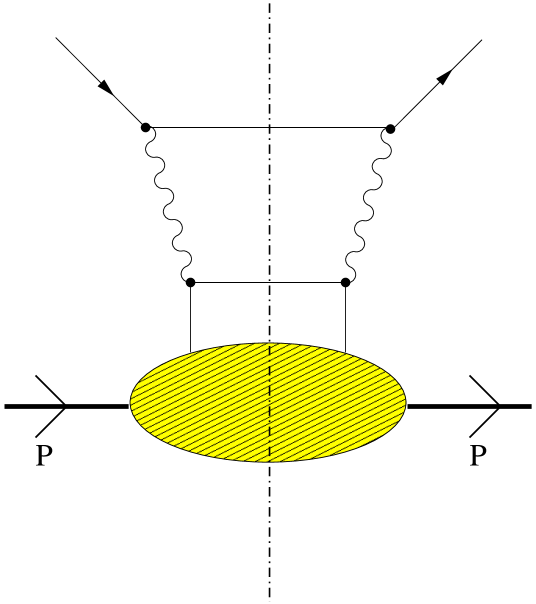
Figure 4: Unitarity diagram in DIS (forward Compton scattering)

The evolution equations describing NFPD’s are known in operatorial form [16]. Single and double parton distributions are obtained sandwiching the operatorial solution with 4 possible types of initial/final states $<p|...|p>,<p|...|0>,<p^{\prime}|...|p>$, corresponding, respectively, to the case of diagonal parton distributions, distribution amplitudes and, in the latter case, skewed and double parton distributions [1, 16]. The ansatz for the general solution of the evolution equations up to next-to-leading order for $H_{q}(x,\xi)$ is given by [7]

$$H_{q}(x,\xi)=\sum_{k=0}^{\infty}\frac{A_{k}(x,\xi)}{k!}\log^{k}\left(\frac{\alpha(Q^{2})}{\alpha(Q_{0}^{2})}\right)+\alpha(Q^{2})\sum_{k=0}^{\infty}\frac{B_{k}(x,\xi)}{k!}\log^{k}\left(\frac{\alpha(Q^{2})}{\alpha(Q_{0}^{2})}\right),$$ (15)

where we have introduced arbitrary scaling coefficients $(A_{k},B_{k})$, now functions of two parameters $(x,\xi)$.

The evolution can be written down in various forms. The one we have exploited comes from kinetic arguments on which we now briefly elaborate.

In the non-forward case (DGLAP-type evolution) the identification of a transition probability for the random walk [7] associated with the evolution of the parton distribution is obtained via the non-forward transition probability

$$w_{\zeta}(x|y) = \frac{\alpha}{\pi}C_{F}\frac{1}{y-x}\left[1+\frac{x}{y}\frac{(x-\zeta)}{y-\zeta}\right]\theta(y>x)$$

$$w^{\prime}_{\zeta}(y|x) = \frac{\alpha}{\pi}C_{F}\frac{x^{2}+y^{2}}{x^{2}(x-y)}\theta(y<x)$$ (16)

and the corresponding master equation is given by

$$\frac{d\mathcal{F}_{q}}{d\tau}=\int_{x}^{1}dy\,w_{\zeta}(x|y)\mathcal{F}_{q}(y,\zeta,\tau)-\int_{0}^{x}dy\,w^{\prime}_{\zeta}(y|x)\mathcal{F}_{q}(x,\zeta,\tau),$$ (17)

that can be re-expressed in a form which is a simple generalization of the formula for the forward evolution [7]

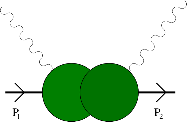
Figure 5: Overlap of wave functions in proton Compton scattering

A Kramers-Moyal expansion of the equation allows to generate a differential equation of infinite order with a parametric dependence on $\zeta$

$$\frac{d\mathcal{F}_{q}}{d\log Q^{2}} = \int_{\alpha(x)}^{0}dy\,w_{\zeta}(x+y|x)\mathcal{F}_{q}(x,\zeta,\tau)+\int_{0}^{-x}dy\,w^{\prime}_{\zeta}(x+y|x)\mathcal{F}_{q}(x,\zeta,\tau)$$ (18)

$$-\sum_{n=1}^{\infty}\int_{0}^{\alpha(x)}dy\frac{(-y)^{n}}{n!}{\partial_{x}}^{n}\left(w_{\zeta}(x+y|x)\mathcal{F}_{q}(x,\zeta,\tau)\right).$$

If we arrest the expansion at the first two terms $(n=1,2)$ we are able to derive an approximate equation describing the dynamics of partons for non-diagonal transitions which is similar to constrained random walks [7].

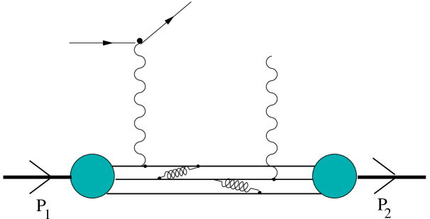
Figure 6: ERBL factorization of proton Compton scattering

2.3 Possible Constraints

Kinetic analogies are an interesting way to test positivity of the evolution for suitable (positive) boundary conditions, though their practical use appears to be modest, since it is limited to leading order in the strong coupling $\alpha_{s}$ [7]. Other interesting constraints emerge also from other studies, based on a unitarity analysis [19], which also may be of help. Their practical impact in the modeling of these distributions has not been studied at all.

We should stress that these QCD bounds, similar to the Soffer bound for $h_{1}$ [13], some of them involving forward and nonforward distributions at the same time, should be analized carefully in perturbation theory. All the anomalous dimensions are known up to next-to-leading order and the study is possible. Another input comes from Ji’s sum rule on angular momentum [1], which needs to be satisfied. One can view Ji’s sum rule also as a constraint between the evolution of angular momentum and the nonforward parton distributions for a vanishing $t$. The evolution of all the distributions, including angular momentum is also known, and there is wide room to play with the boundary conditions. Other constraints may come from a combined sum rule analysis for proton Compton scattering, along the lines suggested in [15]. The soft mechanism based on the overlap of wave functions (see Fig. 5), pre-asymptotic (Fig. 6) may be studied using dispersion theory of 4-current correlators (Fig. 7), especially for scattering at wide angle.

3 EWDVCS

We now come to discuss an interesting generalization of the standard DVCS process.

The electroweak version of the process (EWDVCS), in the regime that we are interested in, requires the notion of electroweak NPD’s to be conveniently described. A charged current version of this interaction, with an electron or a neutrino in the final state, the latter coming from an electron, can also be contemplated. We are going to argue that there are motivations for studying these extensions for astroparticle applications.

If we entertain the possibility of extending DVCS to the weak sector we will be facing the issue of large suppression in the cross section. For charged currents there is a similar BH background, but not for neutral currents, for instance in neutrino-nucleon scattering, this aspect is obviously not present. We shoukd keep in mind that it is very likely that most of our hopes to detect dark matter using ground or underground based facilities, whatever they may be, have to rest considerably on our capability to detect weakly interacting particles of various masses and in various kinematical domains.

Differently from standard accelerator searches, in the astroparticle case the range of these interactions vary from low to high to extremely high energy.

The example of Ultra High Energy Cosmic Rays (UHECR) [24] and the undeterminations associated to the estimates of their energy both in the strong sector (for instance at the Greisen-Ztsepin-Kuzmin (GZK) cutoff and around it for p-p first impacts) and in the weak sector - such as in the detection of neutrino-induced horizontal air showers - are clear examples of a theory that is unable to be fully predictive. We remark that arguments linked to parton saturations and to the small-x impact of the distributions for Ultra High Energy (UHE) neutrino scattering have been formulated only recently and show a considerable readjustment [21] of the UHE cross section. In particular, our overall understanding of this domain is still under debate, especially from the S-matrix perspective [25] Neutrino studies have only been confined to the atmospheric and solar case, for obvious reasons. Though the fluxes may change considerably with a varying energy, it is conceiveable that other cosmic ray experiments may be looking for bounds on the parameter space of the various models which have been recently proposed.

In the search for dark matter it is essential to have an open view on the possible mass range of the possible candidates, including lower mass candidates [22]. While dark matter searches can be rather indirect and can rely on new astronomical searches with excellent perspectives for the future - such as weak gravitational lensing (gravitational shear measurements) or other observational methods having a statistical imprint - [20] weak or superweak interactions are still likely to be studied extensively using nucleon targets. We believe that the few GeV region of QCD has very good chances to be relevant in the astroparticle territory, and for a just cause. One additional photon in the final state plus a recoiling nucleon is a good signal for detecting light dark matter and both the fluxes and the cross sections should be accurately quantified [26].

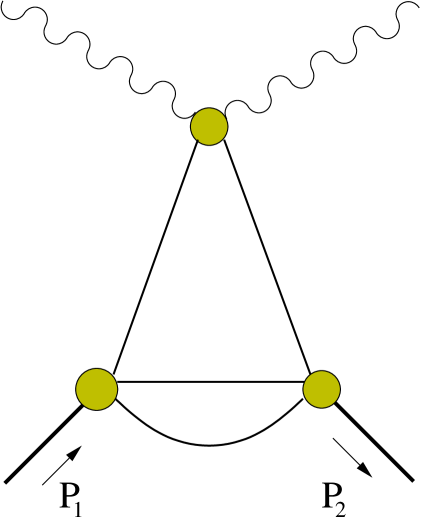
Figure 7: Dispersive Approach to proton Compton scattering using current correlators (above). The spectral density of pion Compton scattering (below).

4 Conclusions

We have illustrated some of the basic features of NFPD’s and we have emphasized that there are other possible applications of the theory, especially in the weak sector, which may be relevant in the astroparticle domain. Any attempt to obtain a complete coverage of neutrinos and dark matter interaction with nucleons in underground experiments should also include searches in the intermediate energy region of QCD with far reaching consequences.

Acknowledgements

C.C. thanks Paolo Amore for collaborating (long ago) on the analysis of the process and Celine Boehm and A. Faraggi for discussions on dark matter searches during a visit at Oxford University, England.

References

- [1] X. Ji, Phys. Rev. D55, 7114 (1997);
- [2] A.V. Radyushkin , Phys. Rev. D 56, 5524 (1997).
- [3] D. Muller, D. Robaschik, B. Geyer, F.-M. Dittes and J. Horejsi, Fortshcr. Phys. 42, 101 (1994).
- [4] J.C. Collins, L. Frankfurt and M. Strikman, Phys.Rev.D56, 2982 (1997).
- [5] A.V. Radyushkin, in M. Shifman (ed.): Boris Ioffe Festschrift ’At the Frontier of Particle Physics / Handbook of QCD’, vol. 2, 1037.
- [6] DVCS@JLAB, Hall A Coll. (J.P. Chen et al.), Proposal to JLAB-Pac-18 (http://www.jlab.org/ sabatie/dvcs); Hermes Coll. (A. Airapetian et al.), Phys.Rev.Lett. 87 182001 (2001) hep-ex/0106068;
- [7] A. Cafarella, C. Corianò and M. Guzzi, Presented at Int. Workshop on Nonlinear Physics II, Jul 2002, hep-ph/0209149
- [8] X. Ji, Phys.Rev.Lett.91, 062001 (2003).
- [9] T. Curtright and C. Zachos, Prog.Theor.Phys.Suppl. 135 244, 1999; J.Phys. A32 771, 1999; C. Zachos, Int.J.Mod.Phys. A17, 2002.
- [10] J. Blumlein, B. Geyer and D. Robaschick, Nucl. Phys B560, 283 (1999); A.V. Belitsky, D. Muller, N. Niedermeier and A. Shäfer, Nucl. Phys. B546, 279 (1999); B. Geyer and M. Lazar, Nucl. Phys. B581, 341 (2000); Phys.Rev.D63, 094003 (2001); M. Lazar, Ph.D. Thesis, Univ. of Leipzig (2002); A.V. Radyushkin and C. Weiss, Phys.Rev. D63, 114012 (2001).
- [11] K.J. Golec-Biernat and A.D. Martin, Phys. Rev. D59 014029 1337 (1999).
- [12] R. L. Jaffe Nucl. Phys B229, 205 (1983).
- [13] J. Soffer, Phys. Rev. Lett. 74, 1292 (1995).
- [14] C. Corianò and H.N. Li and C. Savkli, JHEP 7, 8 (1998).
- [15] C. Corianò, A.V. Radyushkin and G. Sterman, Nucl. Phys B405,481 (1993); C. Corianò, Nucl. Phys. B410, 90, (1993).
- [16] I.I. Balitsky and V.M. Braun, Nucl. Phys. B311, 541 (1989).
- [17] M. Vanderhaeghen, P.A.M. Guichon and M. Guidal, Phys.Rev. D60 094017 (1999);
- [18] A. Freund, M. McDermott and M. Strikman, Phys.Rev. D67, 036001 (2003).
- [19] B. Pire, J. Soffer, O. Teryaev, Eur.Phys.J. C8, 103 (1999).
- [20] P. Schneider, astro-ph/0306465, Proceedings of the 35th Adv. Saas-Fee School on Gravitational Lensing.
- [21] K. Kutak and J. Kwiecinski, hep-ph/0303209.
- [22] C. Boehm and P. Fayet, hep-ph/0305261; C. Boehm, T.A. Ensslin, J. Silk, astro-ph/0208458.
- [23] A. Cafarella, C. Corianò and M. Guzzi hep-ph/0303050; A. Cafarella and C. Corianò, hep-ph 0303050
- [24] A. Cafarella, C. Corianò, A. E. Faraggi, hep-ph/0308169; Proceedings of 15th IFAE, Lecce, April 2003, hep-ph/0306236.
- [25] A.R. White hep-ph/9408259; hep-ph/9804207.
- [26] P. Amore et. al., in preparation.