Measurement of $\alpha_{s}$ and the $\beta$ function with the DELPHI detector at LEP

Abstract

Event shape distributions in $e^{+}e^{-}$ annihilation are determined from the DELPHI data taken between 183 and 207 GeV. From these the strong coupling $\alpha_{s}$ is extracted with several techniques. Together with the results from other LEP2 energies and at about $m_{Z}$ this allows both, a combined measurement of $\alpha_{s}$ and a test of the scale dependence of the strong interaction. Alternatively the renormalisation group invariant (RGI) perturbation theory is applied to measure the $\beta$ function of strong interaction. The results are good agreement with the QCD expectation and allow to exclude the existence of light gluinos with a mass below 30 GeV in a model independent way.

1 Introduction

Neglecting quark masses, $\alpha_{s}$ is the only free parameter of QCD, the theory of strong interaction. Thus its measurement is a task of fundamental importance. Additionally, the scale dependence of the strong coupling, as governed by the $\beta$ function, is among the important predictions of QCD.

This note presents both, a measurements of $\alpha_{s}$ at different LEP2 energies, and a test of the scale dependence of the strong interaction. In both cases several techniques are applied.

From the event shapes Thrust, C parameter, heavy jet mass, wide and total jet broadening, $\alpha_{s}$ is extracted with four different methods: The differential distributions at each energy are compared to predictions in $\cal O$($\alpha_{s}^{2}$), pure NLLA and matched $\cal O$($\alpha_{s}^{2}$)+NLLA, folded with fragmentation models. Furthermore, $\alpha_{s}$ is extracted from the mean values using an analytical power correction ansatz. These measurements, together with the results from other LEP2 energies and about $m_{Z}$, are finally combined into one $\alpha_{s}$ measurement for each method.

The $\beta$ function is extracted with two different techniques: From the $\alpha_{s}$ values directly, and from the energy evolution of mean values of event shapes. The last method is based on the renormalisation group invariant (RGI) perturbation theory [1].

These analyses and the theoretical background are described in more detail in [2, 3] and the references therein.

2 Data and background

The analysis is based on data taken with the DELPHI detector in the years from 1997 to 2000 at centre of mass energies between 183 and 207 GeV. Details on the DELPHI detector and the event selection can be found in [2] and the references therein. In total a number of $\approx$10.000 hadronic events have been analyses. This is less than 1% of the statistics gathered at $\sqrt{s}=m_{Z}$. But not only the cross section at LEP2 is much smaller than at LEP1. Additionally one has to deal with significant background processes. Most important are radiative (ISR) events and the production of W pairs (four fermion events). For details we refer again to [2].

3 Determination of $\alpha_{s}$  from event shape distributions

From the differential distributions of 1-T, C parameter, $M^{2}_{\mathrm{h}}/E^{2}_{\mathrm{vis}}$, $B_{\mathrm{max}}$ and $B_{\mathrm{sum}}$, $\alpha_{s}$ is determined by fitting an $\alpha_{s}$ dependent QCD prediction folded with a hadronisation correction to the data. As QCD predictions $\cal O$($\alpha_{s}^{2}$), pure NLLA, and the combined $\cal O$($\alpha_{s}^{2}$)+NLLA in $\log R$-scheme are employed.

In [4] it has been shown that fixing the renormalisation scale to $\mu^{2}=E_{\mathrm{c}m}^{2}$ results in a marginal description of the data. Therefore, the experimentally optimised scales from [4] are used for the $\cal O$($\alpha_{s}^{2}$) fits. For the NLLA and the combined NLLA+$\cal O$($\alpha_{s}^{2}$) fits, $\mu$ is set equal to $E_{\mathrm{c}m}$.

3.1 Theoretical uncertainties

All perturbative QCD predictions introduce uncertainties due to missing higher orders. The conventional method for its estimation is to consider the effect of a renormalisation scale variation. This method however has at least two drawbacks: Since the scale error is positively correlated with $\alpha_{s}$, this definition produces a bias towards small $\alpha_{s}$ values. Secondly there are indications, that observables calculated from one hemisphere only (like the heavy jet mass or $B_{\mathrm{max}}$) yield less reliable results in the resummation of leading logarithms [5]. This should be reflected in their theoretical errors. In contrary the scale variation yields the smallest uncertainty for the heavy jet mass and especially $B_{\mathrm{m}ax}$. For this reason a new definition of the theoretical uncertainty for the logR prediction was developed. It is based on the additional ambiguity which enters the resumed prediction from the phase space restriction. These calculations are forced to vanish at the kinematic limit $y_{max}$ using the replacement:

$$L=\ln\frac{1}{y}\rightarrow L=\ln\left[\frac{1}{Xy}-\frac{1}{Xy_{max}}+1\right]$$ (1)

Usually $X=1$ is chosen, although different values for this $X$ scale introduce formally only subdominant contributions [6]. The theoretical error is now defined as half of the difference when $X$ is varied between $2/3$ and $3/2$. The same definition of the theoretical uncertainty has been adopted for the pure NLLA prediction.

For the $\cal O$($\alpha_{s}^{2}$) calculation the error from the variation around the experimentally optimized scales is still used, as in previous publications [4, 7].

In order to avoid the above mentioned bias, the corresponding scale variations are calculated from theory distributions with a fixed value of $\alpha_{s}$.

3.2 Combination of the results

For a combination of the $\alpha_{s}$ results from different observables at the same energy a proper treatment of the correlation is mandatory. An average value $\bar{y}$ for correlated measurements $y_{i}$ is:

$$\bar{y}=\sum_{i=1}^{N}w_{i}y_{i}\qquad\mbox{with:}\quad w_{i}=\frac{\sum_{j}(V^{-1})_{ij}}{\sum_{k,l}(V^{-1})_{kl}}$$

The covariance matrix $V$ has an additive structure for each source of uncertainty:

$$V=V^{\mathrm{stat}}+V^{\mathrm{sys.exp.}}+V^{\mathrm{had}}+V^{\mathrm{scale}}$$

The statistical component was estimated with Monte Carlo simulation, while the correlation of systematic errors is modeled by the minimum overlap assumption:

$$V_{ij}=\min(\Delta_{i}^{2},\Delta_{j}^{2})$$ (2)

Here $\Delta_{i}$ denotes the corresponding error of the observable $i$.

4 Determination of $\alpha_{s}$ from mean values with power corrections

The analytical power ansatz is used to determine $\alpha_{s}$ from mean event shapes. This ansatz provides an additive term to the perturbative $\cal O$($\alpha_{s}^{2}$) QCD prediction [8].

$$\left<f\right>=\frac{1}{\sigma_{\mathrm{t}ot}}\int f\frac{df}{d\sigma}d\sigma=\left<f_{\mathrm{p}ert}\right>+\left<f_{\mathrm{p}ow}\right>$$ (3)

Here an additional non–perturbative parameter ${\alpha}_{0}$ enters for the contributions to the event shape below an infrared matching scale $\mu_{I}$. In order to measure $\alpha_{s}$ from individual high energy data the parameter ${\alpha}_{0}$ has to be determined by a global fit of $\alpha_{s}$ and ${\alpha}_{0}$ to a large set of measurements at different energies.

5 Combination of all DELPHI $\alpha_{s}$ measurements

Assuming the validity of the QCD predicted energy dependence of $\alpha_{s}$, all results can be evolved to a reference energy, e.g. $M_{Z}$, and combined to a single $\alpha_{s}$$(M_{Z})$ measurement. We include also the LEP2 results at 133, 161 and 172 GeV from [7]. For $\alpha_{s}$ at and around $M_{Z}$ we have reanalyzed the distributions from [7] for our five observables and combined the results using the same treatment of correlation as described in section 3.2. For $\alpha_{s}$ from mean values the measurements of events with reduced centre–of–mass energy between 44 and 76 GeV [3] have been included as well. In combining the $\alpha_{s}$ results one faces again the problem of correlation. Although the measurements at different energies are obviously statistically independent, the systematic and theoretical errors are not. Again this part of the covariance matrix was modeled assuming minimum overlap. The only difference to the method described in section 3.2 is, that the error of ISR and four fermion background correlates only those measurements which have this source of uncertainty in common.

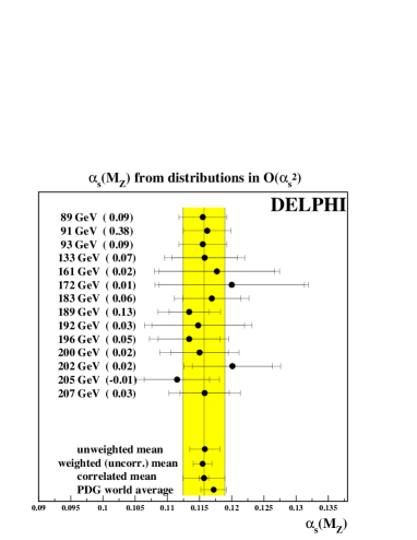
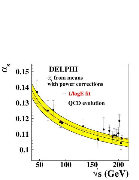
The result of these combinations are given in Table 1. As an example the Figures 1 and 2 display the combination and energy evolution of the $\alpha_{s}$ values from the ${\cal{O}}(\alpha_{s}^{2})$ fit to distributions and from mean values with power corrections respectively.

As can be seen from Table 1 the total errors are dominated by the theoretical uncertainty.

theory	$\alpha_{s}(M_{Z})$	exp.	theo.
${\cal{O}}(\alpha_{s}^{2})$	0.1157	0.0018	0.0027
NLLA	0.1093	0.0023	0.0051
${\cal{O}}(\alpha_{s}^{2})$+NLLA	0.1205	0.0021	0.0050
means	0.1184	0.0009	0.0032

Table 1: Results of combining all DELPHI $\alpha_{s}$ measurements at LEP1 and LEP2. The quoted errors are the experimental (stat. and sys.exp.) and theoretical (scale and hadronisation) ones.

Figure 1: Values for $\alpha_{s}$ at different energies from a fit of the ${\cal{O}}(\alpha_{s}^{2})$ prediction to distributions. Also shown are the results of different mean value definitions. The numbers in brackets give the weights of the individual measurements in the calculation of the correlated average.

Figure 2: Scale dependence of $\alpha_{s}$ from mean values with power corrections. The band displays the QCD energy evolution of the mean value of this measurements. The dotted line indicates the fit of the scale dependence.

Figure 3: Scale dependence of 1/$\langle 1-T\rangle$ together with theoretical predictions in the RGI framework and the fit result.

6 The running of $\alpha_{s}$

In the previous section we have assumed the validity of QCD in order to combine the measurements at different energies. Now we will turn around the perspective and use the determination of $\alpha_{s}$ at different energies to test the predicted scale dependence of the coupling. The logarithmic energy slope of the inverse coupling is (in second order) given by:

$$\frac{\mathrm{d}\alpha_{s}^{-1}}{\mathrm{d}\ln Q}=2b_{0}+2b_{1}\alpha_{s}=\left\{\begin{array}[]{ll}1.27&\mbox{(QCD)}\\ 0.89&\mbox{(QCD+gluinos)}\\ \end{array}\right.$$

Table 2 gives the slopes when fitting the function $1/(b\log{\sqrt{s}}+c)$ to the $\alpha_{s}$ values. Figure 2 displays the fit result for the $\alpha_{s}$ values from mean values with power corrections as an example. The results are in good agreement with the QCD expectation. The unweighted mean of the different measurements yields $1.28\pm 0.12$(RMS). In this fit the correlation between the measurements is taken into account by including the full covariance matrix into the definition of the $\chi^{2}$ function. The correlation is modeled similarly as described in section 3.2. The only differences here are that the statistical errors are uncorrelated, and that the errors from ISR and four fermion background correlate only those data which have these sources of uncertainty in common.

theory	$\frac{d\alpha_{s}^{-1}}{d\log{E_{\mathrm{CM}}}}$ $\pm$ stat $\pm$ sys
${\cal{O}}(\alpha_{s}^{2})$	1.27 $\pm$ 0.15 $\pm$ 0.33
NLLA	1.40 $\pm$ 0.17 $\pm$ 0.44
${\cal{O}}(\alpha_{s}^{2})$+NLLA	1.32 $\pm$ 0.11 $\pm$ 0.27
means (pow.corr.)	1.11 $\pm$ 0.09 $\pm$ 0.19

Table 2: Results for the slope $b$ when fitting the function $1/(b\log{\sqrt{s}}+c)$ to $\alpha_{s}$ values obtained for the different energies.

7 The RGI method

The $\beta$ functions governs not only the scale dependence of $\alpha_{s}$, but directly the energy evolution of e.g. event shapes. In the renormalisation group invariant (RGI) perturbation theory [1] the energy evolution of fully inclusive quantities ${\cal{R}}$, like mean values of event shape distributions, can be used to measure the $\beta$ function directly:

$$Q\frac{dR^{-1}}{dQ}=\frac{\beta_{0}}{2}+\frac{\beta_{1}}{4}R+\cdots=\left\{\begin{array}[]{ll}4.14&\mbox{(QCD)}\\ 2.76&\mbox{(QCD+gluinos)}\\ \end{array}\right.$$

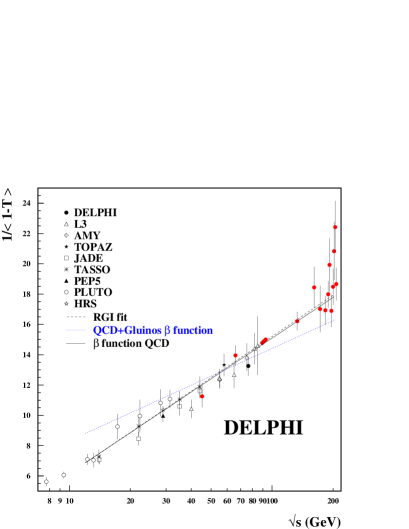
Here $R$ is ${\cal{R}}/A$, with $A$ the first order coefficient when expanding ${\cal{R}}$ in powers of $\alpha_{s}/\pi$. In [3] it was shown, that this approach yields consistent results for various observables. However, the highest accuracy can be achieved for the observable ${\cal{R}}=\langle 1-T\rangle$ , since here the most low energy data is available. Our measurement yields:

$$Q\frac{dR^{-1}}{dQ}=4.21\pm 0.18$$

The fit result is displayed in Figure 3. This is in good agreement with the QCD expectation and allows to exclude the existence of light gluinos in the mass range of $\leq$30 GeV.

References

- [1] A. Dhar, Phys. Lett. B128 (1983) 407
- [2] DELPHI 2002–065 CONF 493 (2002)
- [3] DELPHI 2002–049 CONF 583 (2002)
- [4] DELPHI Coll., P. Abreu et al. E.Phys.J. C14(2000) 557
- [5] E. Gardi and J. Rathsman, hep-ph/0201019
- [6] G. Salam et al, hep-ph/0110213
- [7] DELPHI Coll., P. Abreu et al.,Phys.Lett. B456(1999)397
- [8] Y. L. Dokshitzer et al. Phys.Let. B352 (1995)451