Are $\Theta^{+}$ and the Roper resonance diquark-diquark-antiquark states?

Abstract

We consider a $[ud]^{2}\bar{s}$ current in the QCD sum rule framework to study the mass of the recently observed pentaquark state $\Theta^{+}(1540)$, obtaining good agreement with the experimental value. We also study the mass of the pentaquark $[ud]^{2}\bar{d}$. Our results are compatible with the interpretation of the $[ud]^{2}\bar{d}$ state as being the Roper resonance $N(1440)$, as suggested by Jaffe and Wilczek.

The recent discovery of an exotic baryon with the $K^{+}n$ quantum numbers, the $\Theta^{+}(1540)$ lep ; diana ; clas ; saphir with mass and width compatible with predictions made by Diakonov, Petrov and Polyakov dpp prompted a lively debate about the spectroscopy of non conventional hadronic states jawil ; kali ; hep07 ; zhu . Since the $\Theta^{+}$ cannot be a three quark state and its minimal quark content is $uudd\overline{s}$ one is left with the question of how these quarks are organized. They could be: a) uncorrelated quarks inside a bag strot ; b) a $K-N$ molecule bound by a van-der Waals force brodsky ; c) a “$K-N$” bound state in which $uud$ and $u\overline{s}$ are not separately in color singlet states zhu ; d) a diquark-triquark $(ud)-(ud\overline{s})$ bound state kali and e) a diquark-diquark-antiquark state jawil . In this note we will explore this last possibility, using the QCD sum rules framework to give a more quantitative basis to the semi-qualitative argument presented in jawil .

According to Jaffe and Wilczek (JW), each diquark pair has spin zero and is in the $\bar{\textbf{3}}$ representation of SU(3), in color and flavor. The two diquark pairs combine in a $P$-wave orbital angular momentum to form a 3 state in color, spin $S=0$, and $\bar{\textbf{6}}$ in flavor. The resulting state is then combined with the antiquark to form a flavor antidecuplet $\bar{\textbf{10}}_{f}$ and octet ${\textbf{8}_{f}}$, with spin $S=1/2$. The $\Theta^{+}$ is at the top of the antidecuplet $\bar{\textbf{10}}_{f}$ and has an isospin $I=0$. JW have also interpreted the lightest particle in the octet ${\textbf{8}_{f}}$, $[ud]^{2}\bar{d}$, as the Roper resonance, since it has the same quantum numbers of the nucleon. The Roper resonance is thus identical to the $\Theta^{+}$ except for the substitution of the strange antiquark by a down antiquark. This would explain why the mass difference between $\Theta^{+}(1540)$ and $N(1440)$ is so close to the strange quark mass. It is therefore interesting to verify if this mass splitting can be obtained in a more detailed calculation. In the case of QCD sum rules (QCDSR) there are several contributions from the OPE, involving many operators which account for the nonperturbative dynamics, and thus this simple dependence with $m_{s}$ is not expected a priori. Using the same diquark-diquark-antiquark for the Roper, we will calculate this mass difference.

Among the works on the $\Theta^{+}$ resonance the QCDSR calculation of Zhu zhu is of particular relevance for us. He used the triquark - $q\overline{q}$ configuration with both in the color adjoint representation. In fact, this configuration is the c) in the short list given above. In QCDSR, different configurations are implemented with the use of different interpolating currents. As it will be seen, both currents will give approximately the same mass for the $\Theta^{+}$ but not necessarily the same mass splitting between $\Theta^{+}$ and Roper resonance.

In the QCDSR approach svz ; rry , the short range perturbative QCD is extended by an OPE expansion of the correlators, which results in a series in powers of the squared momentum with Wilson coefficients. The convergence at low momentum is improved by using a Borel transform. The expansion involves universal quark and gluon condensates. The quark-based calculation of a given correlator is equated to the same correlator, calculated using hadronic degrees of freedom via a dispersion relation, providing sum rules from which a hadronic quantity can be estimated. The QCDSR calculation of hadronic masses centers around the two-point correlation function given by

$$\Pi(q)\equiv i\int d^{4}x\,e^{iq\cdot x}\langle 0|T\eta(x)\overline{\eta}(0)|0\rangle\ ,$$ (1)

where $\eta(x)$ is an interpolating field (a current) with the quantum numbers of the hadron we want to study.

Following the JW conjecture jawil , we can write two independent interpolating fields with the quantum numbers of $\Theta^{+}(1540)$:

$$\eta_{1}(x) = {1\over\sqrt{2}}\epsilon_{abc}\left([u_{a}^{T}(x)C\gamma_{5}d_{b}(x)][u_{c}^{T}(x)C\gamma_{5}d_{e}(x)]C\bar{s}^{T}_{e}(x)-(u\leftrightarrow d)\right)\ ,$$ (2)

$$\eta_{2}(x) = {1\over\sqrt{2}}\epsilon_{abc}\left([u_{a}^{T}(x)Cd_{b}(x)][u_{c}^{T}(x)Cd_{e}(x)]C\bar{s}^{T}_{e}(x)-(u\leftrightarrow d)\right)\ ,$$ (3)

where $a,~{}b,~{}c$ and $e$ are color index and $C=-C^{T}$ is the charge conjugation operator. One can check that each diquark pair has spin zero and is in the $\bar{\textbf{3}}$ representation of SU(3) in color and flavor. The total current has isospin zero, positive parity and spin 1/2.

As in the nucleon case, where one also has two independent currents with the nucleon quantum numbers io1 ; dosch , the most general current for $\Theta^{+}$ is a linear combination of the currents given above:

$$\eta(x)=\left[t\eta_{1}(x)+\eta_{2}(x)\right],$$ (4)

with $t$ being an arbitrary parameter. In the case of the nucleon, the interpolating field with $t=-1$ is known as Ioffe’s current io1 . This current maximizes the overlap with the nucleon as compared with the excited states, and minimizes the contribution of higher dimension condensates.

Inserting Eq. (4) into Eq. (1) we obtain

$$\langle 0|T\eta(x)\overline{\eta}(0)|0\rangle=t^{2}\Pi_{11}(x)+2t\left(\Pi_{12}(x)+\Pi_{21}(x)\right)+\Pi_{22}(x)\,$$ (5)

Calling $\Gamma_{1}=\gamma_{5}$ and $\Gamma_{2}=1$ we get

$$\Pi_{ij}(x)=\langle 0|T\eta_{i}(x)\overline{\eta}_{j}(0)|0\rangle=\epsilon_{abc}\epsilon_{a^{\prime}b^{\prime}c^{\prime}}C{S_{e^{\prime}e}^{s}}^{T}(-x)C\left\{-\mbox{ Tr }[\Gamma_{i}S_{bb^{\prime}}(x)\Gamma_{j}CS^{T}_{aa^{\prime}}(x)C]\right.$$

$$\times\mbox{ Tr }[\Gamma_{i}S_{ee^{\prime}}(x)\Gamma_{j}CS^{T}_{cc^{\prime}}(x)C]+\mbox{ Tr }[\Gamma_{i}S_{be^{\prime}}(x)\Gamma_{j}CS^{T}_{cc^{\prime}}(x)C\Gamma_{i}S_{eb^{\prime}}(x)\Gamma_{j}CS^{T}_{aa^{\prime}}(x)C]$$

$$+\mbox{ Tr }[\Gamma_{i}S_{bb^{\prime}}(x)\Gamma_{j}CS^{T}_{ca^{\prime}}(x)C\Gamma_{i}S_{ee^{\prime}}(x)\Gamma_{j}CS^{T}_{ac^{\prime}}(x)C]-\mbox{ Tr }[\Gamma_{i}S_{be^{\prime}}(x)\Gamma_{j}CS^{T}_{ac^{\prime}}(x)C]$$

$$\times\mbox{ Tr }[\Gamma_{i}S_{eb^{\prime}}(x)\Gamma_{j}CS^{T}_{ca^{\prime}}(x)C]-\mbox{ Tr }[\Gamma_{i}S_{ab^{\prime}}(x)\Gamma_{j}CS^{T}_{ea^{\prime}}(x)C\Gamma_{i}S_{ce^{\prime}}(x)\Gamma_{j}CS^{T}_{bc^{\prime}}(x)C]$$

$$-\mbox{ Tr }[\Gamma_{i}S_{ba^{\prime}}(x)\Gamma_{j}CS^{T}_{cb^{\prime}}(x)C\Gamma_{i}S_{ec^{\prime}}(x)\Gamma_{j}CS^{T}_{ae^{\prime}}(x)C]+\mbox{ Tr }[\Gamma_{i}S_{ba^{\prime}}(x)\Gamma_{j}CS^{T}_{ab^{\prime}}(x)C]$$

$$\left.\times\mbox{ Tr }[\Gamma_{i}S_{ce^{\prime}}(x)\Gamma_{j}CS^{T}_{ec^{\prime}}(x)C]+\mbox{ Tr }[\Gamma_{i}S_{bc^{\prime}}(x)\Gamma_{j}CS^{T}_{ae^{\prime}}(x)C]\mbox{ Tr }[\Gamma_{i}S_{ea^{\prime}}(x)\Gamma_{j}CS^{T}_{cb^{\prime}}(x)C]\right\}\;,$$ (6)

where $S_{ab}(x)$ and $S_{ab}^{s}(x)$ are the light and strange quark propagators respectively.

In order to evaluate the correlation function $\Pi(q)$ at the quark level, we first need to determine the quark propagator in the presence of quark and gluon condensates. Keeping track of the terms linear in the quark mass and taking into account quark and gluon condensates, we get yhhk

$$S_{ab}(x) = \langle 0|T[q_{a}(x)\overline{q}_{b}(0)]|0\rangle={i\delta_{ab}\over 2\pi^{2}x^{4}}\hbox to0.0pt{/\hss}{x}-{m_{q}\delta_{ab}\over 4\pi^{2}x^{2}}-{i\over 32\pi^{2}x^{2}}t^{A}_{ab}g_{\rm s}G^{A}_{\mu\nu}(\hbox to0.0pt{/\hss}{x}\sigma^{\mu\nu}+\sigma^{\mu\nu}\hbox to0.0pt{/\hss}{x})$$ (7)

$$- {\delta_{ab}\over 12}\langle{\overline{q}q}\rangle-{m_{q}\over 32\pi^{2}}t^{A}_{ab}g_{\rm s}G^{A}_{\mu\nu}\sigma^{\mu\nu}\ln(-x^{2})+{i\delta_{ab}\over 48}m_{q}\langle{\overline{q}q}\rangle\hbox to0.0pt{/\hss}{x}-{x^{2}\delta_{ab}\over 2^{6}\times 3}\langle{g_{\rm s}\overline{q}\sigma\!\cdot\!{\cal G}q}\rangle$$

$$+ {ix^{2}\delta_{ab}\over 2^{7}\times 3^{2}}m_{q}\langle{g_{\rm s}\overline{q}\sigma\!\cdot\!{\cal G}q}\rangle\hbox to0.0pt{/\hss}{x}-{x^{4}\delta_{ab}\over 2^{10}\times 3^{3}}\langle{\overline{q}q}\rangle\langle{{\displaystyle{g_{\rm s}^{2}G^{2}}}}\rangle\,,$$

where we have used the factorization approximation for the multi-quark condensates, and we have used the fixed-point gauge yhhk .

Lorentz covariance, parity and time reversal imply that the two-point correlation function in Eq. (1) has the form

$$\Pi(q)=\Pi_{1}(q^{2})+\Pi_{q}(q^{2})\hbox to0.0pt{/\hss}{q}\;.$$ (8)

A sum rule for each scalar invariant function $\Pi_{1}$ and $\Pi_{q}$, can be obtained. As in ref. zhu , in this work we focus on the chirality even structure $\Pi_{q}(q^{2})$.

The phenomenological side is described, as usual, as a sum of pole and continuum, the latter being approximated by the OPE spectral density. In order to suppress the condensates of higher dimension and at the same time reduce the influence of higher resonances we perform a standard Borel transform svz :

$$\Pi(M^{2})\equiv\lim_{n,Q^{2}\rightarrow\infty}\frac{1}{n!}(Q^{2})^{n+1}\left(-\frac{d}{dQ^{2}}\right)^{n}\Pi(Q^{2})$$ (9)

($Q^{2}=-q^{2}$) with the squared Borel mass scale $M^{2}=Q^{2}/n$ kept fixed in the limit.

After Borel transforming each side of $\Pi_{q}(Q^{2})$ and transferring the continuum contribution to the OPE side we obtain the following sum rule at order $m_{s}$:

$$\lambda_{\Theta}^{2}e^{-m_{\Theta}^{2}/M^{2}} = {3c_{1}\over 2^{11}\times 7!~{}\pi^{8}}M^{12}E_{5}+{m_{s}\langle{\bar{s}s}\rangle c_{1}\over 2^{10}\times 5!~{}\pi^{6}}M^{8}E_{3}+{\langle{{\displaystyle{g_{\rm s}^{2}G^{2}}}}\rangle c_{2}\over 2^{15}\times 5!~{}\pi^{8}}M^{8}E_{3}$$ (10)

$$+ {\langle{\overline{q}q}\rangle^{2}c_{3}\over 2^{9}\times 3^{2}~{}\pi^{4}}M^{6}E_{2}-{m_{s}\langle{g_{\rm s}\bar{s}\sigma\!\cdot\!{\cal G}s}\rangle c_{1}\over 2^{14}\times 3^{2}~{}\pi^{6}}M^{6}E_{2}$$

$$+ {m_{s}\langle{\bar{s}s}\rangle\langle{\overline{q}q}\rangle^{2}c_{3}\over 2^{6}\times 3^{2}~{}\pi^{2}}M^{2}E_{0}+{\langle{\overline{q}q}\rangle^{4}c_{1}\over 6^{3}}\,,$$

where $c_{1}=5t^{2}+2t+5$, $c_{2}=(1-t)^{2}$, $c_{3}=7t^{2}-2t-5$ and we have defined

$$E_{n}\equiv 1-e^{-s_{0}/M^{2}}\sum_{k=0}^{n}\left(s_{0}\over M^{2}\right)^{k}{1\over k!}\ ,$$ (11)

which accounts for the continuum contribution with $s_{0}$ being the continuum threshold io1 .

To extract the $\Theta^{+}$ mass, $m_{\Theta}$, we take the derivative of Eq. (10) with respect to $M^{-2}$ and divide it by Eq. (10).

The interpolating field for $N^{+}$ is also given by Eq. (4), just by changing $\bar{s}$ by $\bar{d}$ in Eqs. (2) and (3). Therefore, the sum rule for $N^{+}$ can be obtained from the sum rule in Eq. (10) by neglecting the terms proportional to $m_{s}$.

In the complete theory, the mass extracted from the sum rule should be independent of the Borel mass $M^{2}$. However, in a truncated treatment there will always be some dependence left. Therefore, one has to work in a region where the approximations made are supposedly acceptable and where the result depends only moderately on the Borel variables.

In the numerical analysis of the sum rules, the values used for the strange quark mass and condensates are: $m_{s}=0.15\,\nobreak\,\mbox{GeV}$, $\langle{\overline{q}q}\rangle=\,-(0.23)^{3}\,\nobreak\,\mbox{GeV}^{3}$, $\langle\overline{s}s\rangle\,=0.8\langle{\overline{q}q}\rangle$, $\langle{g_{\rm s}\bar{s}\sigma\!\cdot\!{\cal G}s}\rangle=m_{0}^{2}\langle{\bar{s}s}\rangle$ with $m_{0}^{2}=0.8\,\nobreak\,\mbox{GeV}^{2}$ and $\langle{{\displaystyle{g_{\rm s}^{2}G^{2}}}}\rangle=0.5~{}\nobreak\,\mbox{GeV}^{4}$.

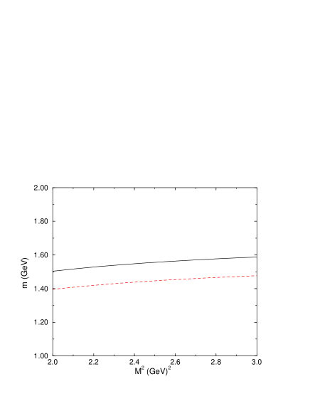
Figure 1: The masses of the pentaquarks $\Theta^{+}$ (solid line) and $N^{+}$ (dashed line)as a function of the Borel parameter $M^{2}$.

We evaluate our sum rules in the range $2.0\leq M^{2}\leq 3.0\nobreak\,\mbox{GeV}^{2}$. In Fig. 1 we show the masses of the pentaquarks $\Theta^{+}$ and $N^{+}$, as a function of the Borel mass using $s_{0\Theta}=(1.5+0.5)^{2}~{}\nobreak\,\mbox{GeV}^{2}=4.0~{}\nobreak\,\mbox{GeV}^{2}$, $s_{0N}=(1.4+0.5)^{2}~{}\nobreak\,\mbox{GeV}^{2}=3.6~{}\nobreak\,\mbox{GeV}^{2}$ and the current parameter in Eq. (4), $t=-1$. We can see that the results are reasonably stable as a function of the Borel mass in the considered interval, and that the values obtained for the masses are in agreement with the experimental values $m_{\Theta}=1540~{}\nobreak\,\mbox{MeV}$ and $m_{\rm{Roper}}=1440~{}\nobreak\,\mbox{MeV}$. Therefore, from our results, it is really possible that the Roper resonance can be identified with the pentaquark $[ud]^{2}\bar{d}$, as suggested by Jaffe and Wilczek jawil . It is very important to mention that the only free parameters in our calculations are the continuum thresholds and the current parameter, and that we have just used the most conventional values for these parameters : $s_{0}=(m+0.5~{}\nobreak\,\mbox{GeV})^{2}$ and $t=-1$. Therefore, the fact that the masses obtained for both cases are in agreement with the experimental results can not be underestimated.

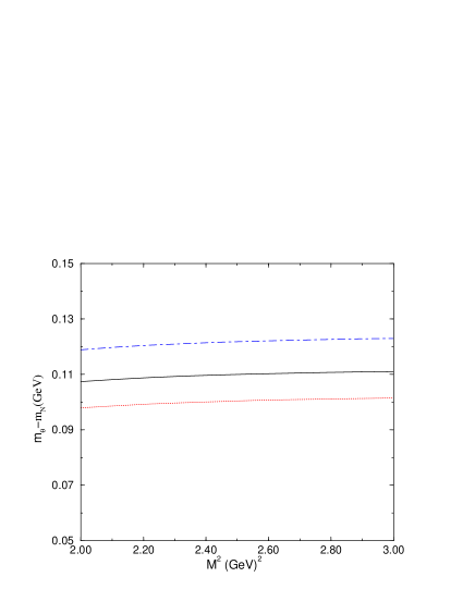
Figure 2: $s_{0}$ dependence of the mass difference. The solid, dot-dashed and dotted lines give $m_{\Theta}-m_{N}$ for $s_{0\Theta}=4.0~{}\nobreak\,\mbox{GeV}^{2}$ and $s_{0N}=3.6~{}\nobreak\,\mbox{GeV}^{2}$, $s_{0\Theta}=3.6~{}\nobreak\,\mbox{GeV}^{2}$ and $s_{0N}=3.2~{}\nobreak\,\mbox{GeV}^{2}$, and $s_{0\Theta}=4.4~{}\nobreak\,\mbox{GeV}^{2}$ and $s_{0N}=4.0~{}\nobreak\,\mbox{GeV}^{2}$ respectively.

In Fig. 2 we show the mass difference, $m_{\Theta}-m_{N}$, as a function of the Borel mass, for different values of the continuum thresholds but keeping $t=-1$. We consider continuum thresholds in the ranges $3.6~{}\nobreak\,\mbox{GeV}^{2}\leq s_{0\Theta}\leq 4.4~{}\nobreak\,\mbox{GeV}^{2}$ and $3.2~{}\nobreak\,\mbox{GeV}^{2}\leq s_{0N}\leq 4.0~{}\nobreak\,\mbox{GeV}^{2}$. The effect of increasing (decreasing) the continuum threshold is to increase (decrease) the masses, however, the increase (decrease) in the $N^{+}$ mass is bigger than in the $\Theta^{+}$ mass, leading to the opposite behavior in the mass difference. For all values considered we can see that the mass difference is of order of $100~{}\nobreak\,\mbox{MeV}$.

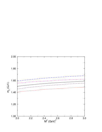
Figure 3: $s_{0}$ and $t$ dependence of $m_{\Theta}$. The solid, dotted and long-dashed lines give $m_{\Theta}$ for $s_{0\Theta}=4.0~{}\nobreak\,\mbox{GeV}^{2}$, $s_{0\Theta}=3.6~{}\nobreak\,\mbox{GeV}^{2}$ and $s_{0\Theta}=4.4~{}\nobreak\,\mbox{GeV}^{2}$ respectively and $t=-1$. The dot-dashed and dashed lines give $m_{\Theta}$ for $t=-0.8$ and $t=-1.1$ respectively and $s_{0\Theta}=4.0~{}\nobreak\,\mbox{GeV}^{2}$.

The effect of changing the current parameter, $t$, is similar to the effect of changing the continuum threshold. In Fig. 3 we show the mass of $\Theta^{+}$ for different values of the continuum threshold and the current parameter. Decreasing the value of $t$ (in modulus) increases the value of both masses keeping the difference approximately constant. In Fig. 3 we show an example with $t=-0.8$, but $t$ can be even smaller without leading to a big change in the masses. For $t=-0.5$, for example, we still have a value that is close to the result for $t=-1$ and $s_{0\Theta}=4.4~{}\nobreak\,\mbox{GeV}^{2}$ (the upper curve in Fig. 3). Increasing $t$ has a stronger effect in decreasing the masses, the effect being even bigger for $\Theta^{+}$. For $t=-1.2$ for instance, the mass difference is only of order of $60~{}\nobreak\,\mbox{MeV}$ and for $t=-1.3$ it is negative.

Fixing $M^{2}=2.5~{}\nobreak\,\mbox{GeV}^{2}$ and considering the ranges $3.6~{}\nobreak\,\mbox{GeV}^{2}\leq s_{0\Theta}\leq 4.4~{}\nobreak\,\mbox{GeV}^{2}$, $3.2~{}\nobreak\,\mbox{GeV}^{2}\leq s_{0N}\leq 4.0~{}\nobreak\,\mbox{GeV}^{2}$ and $-1.1\leq t\leq-0.8$ our results for both pentaquark masses are

$$m_{\Theta}=1.55\pm 0.10~{}\nobreak\,\mbox{GeV},\;\;\;\;\;\;\;\;m_{N}=1.44\pm 0.11~{}\nobreak\,\mbox{GeV}\,,$$ (12)

and $m_{\Theta}-m_{N}=110\pm 10~{}\nobreak\,\mbox{MeV}$, in a very good agreement with the experimental result.

In zhu the value of $M_{0}=1.56\pm 0.15\nobreak\,\mbox{GeV}$ was found for the isoscalar pentaquark, in agreement both with experiment and with our QCDSR calculation. In contrast to our result, the sum rule obtained in zhu does not depend on the strange quark mass $m_{s}$. As a consequence, the substitution $s\rightarrow d$ would only change the quark condensates ( $\langle\overline{s}s\rangle\rightarrow\langle\overline{q}q\rangle$) producing a minor change in the pentaquark masses. This suggests that $N^{+}$ and $\Theta^{+}$ would have a smaller mass difference than we find here.

In conclusion, we have presented a QCD sum rule study of the $\Theta^{+}$ and $N^{+}$ pentaquarks masses using the scheme proposed by Jaffe and Wilczek, according to which both resonances are diquark-diquark-antiquark states. Using our interpolating current we were able to reproduce the experimental value of the $\Theta^{+}(1540)$ and we obtained a mass for the $N^{+}$ which is compatible with the interpretation of this state as the Roper resonance $N(1440)$. We studied the mass difference between these states as a function of the continuum threshold and the current parameter, obtaining $m_{\Theta}-m_{N}\simeq 100~{}\nobreak\,\mbox{MeV}$.

The difference in the sum rules for $\Theta^{+}$ and $N^{+}$ can be entirely assigned to the strange quark mass. This finding supports the analysis performed in jawil and encourages us to calculate the masses of the other antidecuplet members, in particular the masses of the states $\Xi^{+}$ and $\Xi^{--}$. The mass of these states has been estimated to be $\sim 2070~{}\nobreak\,\mbox{MeV}$ in ref. dpp and $\sim 1750~{}\nobreak\,\mbox{MeV}$ in ref. jawil . A QCDSR calculation may be useful in discriminating between the two approaches.

Acknowledgements: This work has been supported by CNPq and FAPESP (Brazil).

References

(1) T. Nakano et al., LEPS Coll., Phys. Rev. Lett. 91,
012002 (2003).
(2) V. Barmin et al., DIANA Coll., hep-ex/0304040.
(3) S. Stepanyan et al., CLAS Coll., hep-ex/0307018.
(4) J. Barth et al., SAPHIR Coll., hep-ex/0307083.
(5) D. Diakonov, V. Petrov, M.V. Polyakov, Z. Phys. A359,
305 (1997).
(6)
R. Jaffe and F. Wilczek, hep-ph/0307341.
(7)
M. Karliner and H. Lipkin, hep-ph/0307243.
(8)
H. Walliser and V. Kopeliovich, hep-ph/0304058;
J. Randrup, hep-ph/0307042;
M. Praszalowicz, hep-ph/0308114;
D. Borisyuk, M. Faber, and A. Kobushkin, hep-ph/0307370;
F. Stancu and D. Riska, hep-ph/0307010;
A. Hosaka, hep-ph/0307232;
P. Bicudo and G. Marques, hep-ph/0308073;
S. Nussinov, hep-ph/0307357;
B. Wybourne, hep-ph/0307170;
C. Carlson, C. Carone, H. Kwee, and V. Nazaryan, hep-ph/0307396;
X. Chen, Y. Mao, and B. Ma, hep-ph/0307381;
S. Capstick, P. Page, and W. Roberts, hep-ph/0307019;
K. Cheung, hep-ph/0308176.
(9)
S.-L. Zhu, hep-ph/0307345;
(10) D. Strotman, Phys. Rev. D20, 748 (1979).
(11) This configuration was considered in the case of
a state in: S.J. Brodsky, I. Schmidt, G.F. de Teramond,
Phys. Rev. Lett. 64, 1011 (1990).
(12) M.A. Shifman, A.I. and Vainshtein and V.I. Zakharov,
Nucl. Phys. B147, 385 (1979).
(13) L.J. Reinders, H. Rubinstein and S. Yazaki, Phys.
Rep. 127, 1 (1985).
(14) B. L. Ioffe, Nucl. Phys. B188, 317 (1981);
B191, 591(E) (1981).
(15) Y. Chung, H. G. Dosch, M. Kremer, D. Schall,
Phys. Lett. B102, 175 (1981);
Nucl. Phys. B197, 55 (1982).
(16) K.-C. Yang et al., Phys. Rev. D47, 3001 (1993).