The radiative return at $\boldsymbol{\Phi}$- and $\boldsymbol{B}$-factories:
FSR at next-to-leading order

Abstract

The measurement of the pion form factor and, more generally, of the cross section for electron–positron annihilation into hadrons through the radiative return has become an important task for high luminosity colliders such as the $\Phi$- or $B$-meson factories. For detailed understanding and analysis of this reaction, the construction of a Monte Carlo program, PHOKHARA, has been undertaken. Version 2.0 was based on a next-to-leading order (NLO) treatment of the corrections from initial-state radiation (ISR). In the present paper a further extension of PHOKHARA (version 3.0) is described, which incorporates NLO corrections to final-state radiation (FSR). The impact of combined ISR and FSR on various distributions is investigated and methods are presented, which will allow the extraction of the form factor, and even give access to inclusive photon emission due to FSR. The dependence of the results on the model for FSR is discussed and the impact of this contribution on the anomalous magnetic moment of the muon is evaluated.

1 Introduction

Electron–positron annihilation into hadrons is one of the basic reactions of particle physics, crucial for the understanding of hadronic interactions. At high energies, around the $Z$ resonance, the measurement of the inclusive cross section and its interpretation within perturbative QCD CKK ; HS give rise to one of the most precise and theoretically founded determinations of the strong coupling constant $\alpha_{s}$ EWG . Also, measurements in the intermediate energy region, between 3 GeV and 11 GeV can be used to determine $\alpha_{s}$ and at the same time give rise to precise measurements of charm and bottom quark masses KS . The low energy region is crucial for predictions of the hadronic contributions to $a_{\mu}$, the anomalous magnetic moment of the muon, and to the running of the electromagnetic coupling from its value at low energy up to $M_{Z}$ (for reviews see e.g. a_mu1 ; Jegetc. ; Melnikov:2001uw ; Davier:2002dy ; HMNT02 ; the most recent experimental result for $a_{\mu}$ is presented in Bennet ). Last, but not least, the investigation of the exclusive final states at large momenta allows for tests of our theoretical understanding of form factors within the framework of perturbative QCD. Beyond the intrinsic interest in this reaction, these studies may provide important clues for the interpretation of exclusive decays of B-mesons, a topic of evident importance for the extraction of CKM matrix elements.

Measurements of the cross section for electron–positron annihilation were traditionally performed in the scanning mode, i.e. by varying the beam energies of the collider. The recent advent of $\Phi$- and $B$-meson factories with enormous luminosities allows us to exploit the radiative return to explore the whole energy region from threshold up to the nominal energy of the collider. Photon radiation from the initial state reduces the cross section by a factor ${\cal O}(\alpha/\pi)$. However, this is easily compensated by the enormous luminosity of ‘factories’ and the advantage of performing the measurement over a wide range of energies in one homogeneous data sample Binner:1999bt (for an early proposal along these lines, see Zerwas ). In principle the reaction $e^{+}e^{-}\to\gamma+{\mathrm{hadrons}}$ receives contributions from both initial- and final-state radiation. Only the former is of interest for the radiative return; the latter has to be eliminated by suitably chosen cuts. The proper analysis thus requires the construction of Monte Carlo event generators. The event generator EVA was based on a leading order treatment of ISR and FSR, supplemented by an approximate inclusion of additional collinear radiation based on structure functions and included two-pion Binner:1999bt and four-pion final states Czyz:2000wh . Subsequently the event generator PHOKHARA was developed; it is based on a complete next-to-leading order (NLO) treatment of ISR Rodrigo:2001jr ; Rodrigo:2001cc ; Rodrigo:2001kf ; Kuhn:2002xg ; Czyz:2002np ; Kuhn:2001 ; Rodrigo:2002hk . In its version 2.0 it included ISR at NLO and FSR at leading order (LO) for $\pi^{+}\pi^{-}$ and $\mu^{+}\mu^{-}$ final states (and four-pion final states without FSR in the formulation described in detail in Czyz:2000wh ).

Recent preliminary experimental results indeed demonstrate the power of the method and seem to indicate that a precision of one per cent or better is within reach CDKMV2000 ; Adinolfi:2000fv ; Aloisio:2001xq ; Denig:2001ra ; babar ; Barbara:Morion ; Berger:2002mg ; Venanzoni:2002 ; Achim:radcor02 ; KLOE:2003 ; Blinov ; Juliet . In view of this progress a further improvement of our theoretical understanding seems to be required. In the present work we therefore present a new version (version 3.0) of PHOKHARA, which allows for the ‘simultaneous’ emission of one photon from the initial and one photon from the final state, requiring only one of them to be hard. This includes in particular the radiative return to $\pi^{+}\pi^{-}(\gamma)$ and thus the measurement of the (one-photon) inclusive $\pi^{+}\pi^{-}$ cross section. The new version of PHOKHARA and various tests of its technical precision will be presented and several suggestions for a model-independent extraction of the form factor will be discussed.

The issue of photon radiation from the final states is closely connected to the question of $\pi^{+}\pi^{-}(\gamma)$ contributions to $a_{\mu}$ (for related discussions, see e.g. Melnikov:2001uw ; Gluza:rad ). Soft photon emission is clearly described by the point-like pion model. Hard photon emission, with $E_{\gamma}\geq{\cal O}$(100 MeV), however, might be sensitive to unknown hadronic physics. We will therefore study the size of virtual, soft and hard corrections separately, and argue that contributions from the hard region, above 100 MeV, are small with respect to the present experimental and theory-induced uncertainty.

The outline of the present paper is the following. In section 2 we recall the basic aspects of the radiative return in leading order, define strategies to separate ISR and FSR through cuts, and discuss their markedly different angular distribution and the characteristic feature of ISR–FSR interference. In section 3 we present the estimate of $\pi^{+}\pi^{-}(\gamma)$ contributions to $a_{\mu}$. Section 4 is devoted to the description of the additional two-photon corrections originating from simultaneous ISR–FSR emission and their implementation in PHOKHARA 3.0. The impact of these new terms on various distributions is described in section 5. A brief summary and our conclusions can be found in section 6.

2 ISR versus FSR and the radiative return at leading order

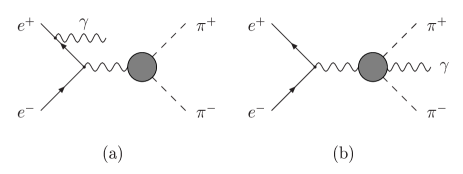
Figure 1: Leading order contributions to the reaction $e^{+}e^{-}\to\pi^{+}\pi^{-}\gamma$ from ISR (a) and FSR (b).

Let us, in a first step, recall the basic ingredients for a proper exploitation of the enormous luminosity at $\Phi$- and $B$-meson factories through the radiative return. In this paper we will concentrate on the measurement of the $\pi^{+}\pi^{-}$ final state, accompanied by one or two photons. We shall start with a discussion of the leading process, with only one photon, radiated from the electron (positron) or the hadronic system:

$$e^{+}\ e^{-}\to\pi^{+}(p^{+})\ \pi^{-}(p^{-})\ \gamma~{}.$$ (1)

For the radiative return this corresponds to the Born approximation, and higher order corrections will be discussed below. The amplitude of interest describes radiation from the initial state (ISR) and is depicted in Fig. 1a (permutations of photon lines will always be omitted). It is proportional to the pion form factor, evaluated at $Q^{2}=(p^{+}+p^{-})^{2}$. However, radiation from the charged pions (FSR) (Fig. 1b) evidently leads to the same final state and must be suppressed and controlled with sufficient precision. A variety of methods, which have already been described in Binner:1999bt ; Rodrigo:2001kf ; Czyz:2002np , will be recalled in the following.

The fully differential cross section describing photon emission can be split into three pieces

$$d\sigma=d\sigma_{\mathrm{ISR}}+d\sigma_{\mathrm{FSR}}+d\sigma_{\mathrm{INT}}~{},$$ (2)

which originate from the squared ISR and FSR amplitudes respectively, plus the interference term. They depend on two Dalitz variables, which characterize the energies of $\pi^{+}$ and $\pi^{-}$ and the photon, and on the three Euler angles describing the orientation of the $\pi^{+}\pi^{-}\gamma$ production plane in the centre-of-mass system (cms). The dependence on the azimuthal angle around the beam direction is trivial in the case of unpolarized beams.

The interference term, $d\sigma_{\mathrm{INT}}$, is antisymmetric under the exchange of $\pi^{+}$ and $\pi^{-}$ or $e^{+}$ and $e^{-}$. This allows us to test the model for FSR and, furthermore, can even lead to a measurement of the amplitude $A_{\mathrm{FSR}}$. The usefulness of this method has already been emphasized in Binner:1999bt .

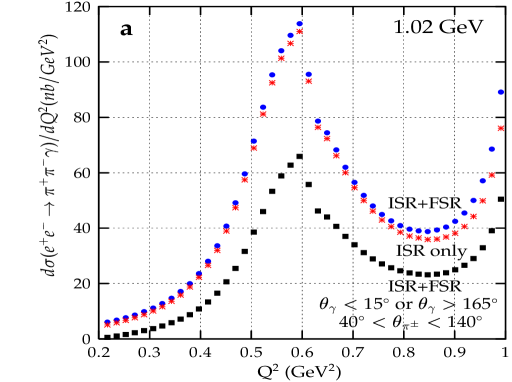
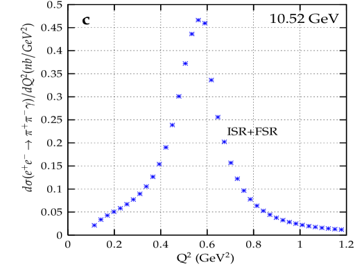
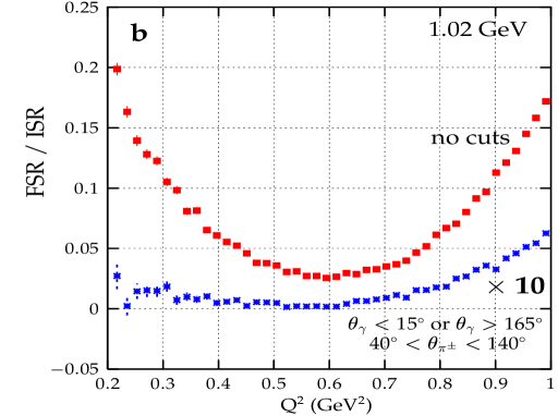
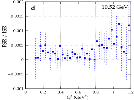
Figure 2: Contributions to the inclusive photon spectrum from ISR compared to ISR plus FSR at $\sqrt{s}~{}=$ 1.02 GeV (a) (without and with cuts) and $\sqrt{s}~{}=$ 10.52 GeV (c). In (b) and (d) the relative contribution of FSR is plotted (multiplied by a factor of 10 for $\sqrt{s}~{}=$ 1.02 GeV, when cuts are applied).

Let us, for the moment, concentrate on the charge-symmetric pieces. The inclusive photon spectrum, separated according to ISR and FSR, is shown in Fig. 2. The discrimination between ISR and FSR is based on the markedly different angular distribution of the photon. Without any assumption on the nature of FSR, the cross section can be written in the form

$$Q^{2}\frac{d\sigma}{dQ^{2}d\cos\theta_{\gamma}} = \frac{4\alpha^{3}}{3s}|F(Q^{2})|^{2}\frac{\beta^{3}(s)}{4}$$ (3)

$$\times \bigg{[}\frac{(s^{2}+Q^{4})}{s(s-Q^{2})}\frac{1}{1-\cos^{2}\theta_{\gamma}}-\frac{s-Q^{2}}{2s}\bigg{]}$$

$$\kern-35.0pt+ \kern-20.0ptA_{1}(s,Q^{2})\cos^{2}\theta_{\gamma}+A_{2}(s,Q^{2})\sin^{2}\theta_{\gamma}~{},$$

where $Q^{2}$ is the invariant mass of the $\pi^{+},\pi^{-}$ system, $\theta_{\gamma}$ is the photon polar angle and $\beta(s)=\sqrt{1-4m_{\pi}^{2}/s}$. Terms $\sim m_{e}^{2}/s$ are neglected for simplicity, while they are present in the program. Fitting the observed photon distribution to this form allows an unambiguously separation of ISR and FSR. The composition of the angular distribution of photons from the two components is displayed in Fig. 3 for three photon energies.

The second option is based on the fact that FSR is dominated by photons collinear to $\pi^{+}$ or $\pi^{-}$, ISR by photons collinear to the beam direction. This suggests that we should consider only events with photons well separated from the charged pions and preferentially close to the beam Binner:1999bt ; Rodrigo:2001kf ; Czyz:2002np . The contamination of the events with FSR is reduced to less than five per mille (Fig. 2b). Considering just the inclusive photon distribution, without inclusion of any cut would necessarily have led us to wrong conclusions. For higher beam energies, the LO FSR is naturally suppressed and at $\sqrt{s}$ = 10.52 GeV it is entirely negligible (Fig. 2d).

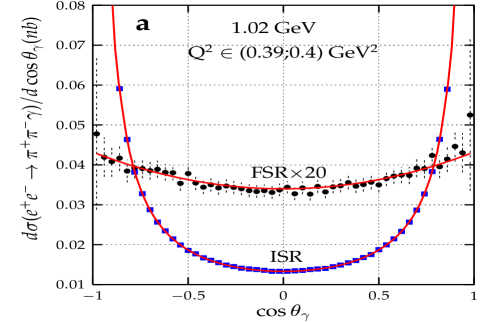
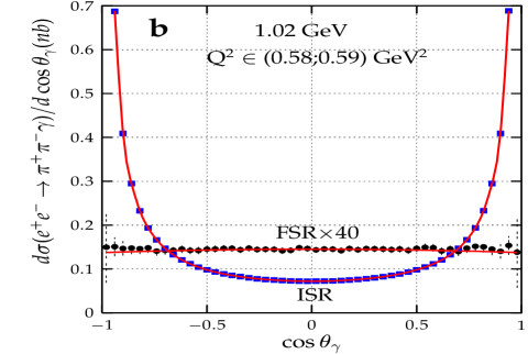
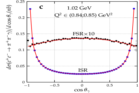
Figure 3: Angular distribution of photons with $E_{\gamma}\in(314,319)$ MeV (a), $E_{\gamma}\in(221,226)$ MeV (b) and $E_{\gamma}\in(93,98)$ MeV (c), separated according to ISR and FSR. The curves represent the fits according to Eq. (3).

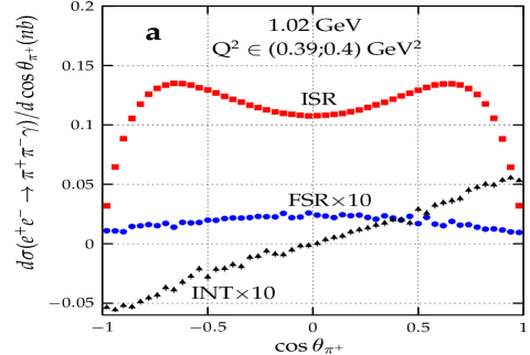
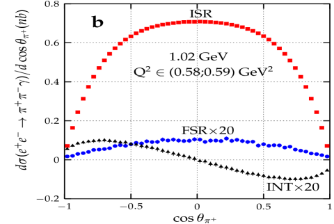
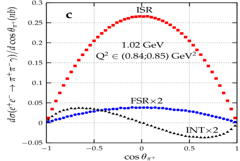
Figure 4: Contributions of ISR, FSR and INT terms to pion polar angle differential cross section for three different ranges of $Q^{2}$.

The interference term is asymmetric under the exchange of $\pi^{+}$ and $\pi^{-}$ or electron and positron:

$$d\sigma_{\mathrm{INT}}(p^{+},p^{-})=-d\sigma_{\mathrm{INT}}(p^{-},p^{+}).$$ (4)

This gives rise to a forward–backward asymmetry of the inclusive pion distribution Binner:1999bt . In kinematical regions where FSR is relatively more pronounced, the interference term is relatively large (Fig. 4c, $Q^{2}$ between 0.84 and 0.85 GeV²) and vice versa (Figs. 4a and 4b). Note that all these considerations refer to the low energy analysis of KLOE. At high energies, e.g. at $B$-factories, ISR and FSR are clearly separate for the $\pi^{+}\pi^{-}\gamma$ final state.

Similar tests were already performed by KLOE Aloisio:2001xq , where it was demonstrated that inclusive photon asymmetries are in excellent agreement with the EVA MC Binner:1999bt , where FSR emission is modelled by point-like pions. Given enough statistics, the charge-asymmetric piece of the cross section can even be investigated for every point in the Dalitz plane, e.g. as a function of $Q^{2}$ and the angle between $\pi^{+}$ and $\gamma$ separately. Keeping these variables fixed and varying the angle between photon and electron, the relative amount of the ISR amplitude can be varied drastically, while the FSR amplitude stays roughly constant.

Alternatively, we could formulate the angular distributions in terms of independent helicity amplitudes for FSR, which depend on the two Dalitz variables only, and deduce information on these amplitudes from their interference with the ISR amplitude. In the absence of any model for FSR beyond scalar QED (sQED) and in view of the fact that sQED will presumably provide a satisfactory description at DAΦNE  energies we shall not dwell further on this subject.

Let us summarise the main points of this ‘leading order’ discussion:

• The cross sections for photon emission from ISR and FSR can be disentangled as a consequence of the marked difference in angular distributions between the two processes, Eq. (3). This observation is completely general and does not rely on any model like sQED for FSR. This allows us to measure the cross section for $\sigma(e^{+}e^{-}\to\gamma^{*}\to\pi^{+}\pi^{-}\gamma)$ directly for fixed $s$ as a function of $E_{\gamma}$, an important ingredient in the analysis of hadronic contributions to $a_{\mu}$, as discussed in Section 3. Alternatively we can employ suitable angular cuts to separate the two components.

• Various charge-asymmetric distributions can be used for independent tests of the FSR model amplitude, with the forward–backward asymmetry as simplest example. Typically the charge asymmetry is large in the region where ISR and FSR are comparable in size and small when the separation is clean and simple from general considerations. A typical case for this second possibility is the radiative return at $\sqrt{s}=10.52$ GeV, at the $B$-meson factories, where the $\pi^{+}\pi^{-}\gamma$ final state is completely dominated by ISR.

3 Higher order contributions to the anomalous magnetic moment of the muon

In leading order the invariant mass of the $\pi^{+}\pi^{-}\gamma$ system is restricted to the cms energy $\sqrt{s}$. If the relevant angular distributions, as predicted by sQED, coincide with the experimental analysis, the validity of this model at lower energies is highly plausible. Nevertheless, a measurement of $\gamma^{*}\to\pi^{+}\pi^{-}\gamma$ for variable $\sqrt{s}$ is desirable for an independent cross check. In Section 4 we will demonstrate that this is indeed possible with the radiative return, if events with two photons in the final state are investigated. This is in fact one of the motivations for extending the event generator PHOKHARA to events with simultaneous ISR and FSR. However, before discussing this issue in detail, an investigation of $\gamma^{*}\to\pi^{+}\pi^{-}\gamma$, the corresponding virtual corrections and the relevance of these amplitudes to the analysis of the muon anomalous magnetic moment $a_{\mu}$ is in order.

Let us concentrate on the one-particle irreducible hadronic contributions

$$a_{\mu}^{\mathrm{had,LO}}=\frac{\alpha^{2}}{3\pi^{2}}\int_{4m_{\pi}^{2}}^{\infty}\frac{ds}{s}\;K(s)\;R(s)\ \ ,$$ (5)

with the familiar kernel $K$ and the $R$ ratio defined through

$$R(s)\propto|\langle 0|J_{\mu}|\mathrm{had},(\gamma)\rangle|^{2}.$$ (6)

$R(s)$ can be obtained from the cross section for electron–positron annihilation into hadrons, after correcting for ISR and for the modifications of the photon propagator, which are sometimes (not quite correctly in the time-like region) summarized as ‘running’ of the fine structure constant.

At the present level of precision of hadronic contributions to $a_{\mu}$, roughly half to one per cent, photonic corrections to final states with hadrons start to become relevant. Qualitatively the order of magnitude of this effect can be estimated either by using the quark model with $m_{u}\approx m_{d}\approx m_{s}\approx 180$ MeV (adopted to describe the lowest order contribution piv ), or with $m_{u}\approx m_{d}\approx m_{s}\approx 66$ MeV (adopted to describe the lowest order contribution to $\alpha(M_{Z})$) or by using $\pi^{+}\pi^{-}$ as dominant intermediate hadronic state plus photons coupled according to sQED. The three estimates (see also Melnikov:2001uw )

$$\delta a_{\mu}({\rm quark},\gamma,m_{q}=180~{}{\rm MeV})=\ 1.880\times 10^{-10}~{},$$

$$\delta a_{\mu}({\rm quark},\gamma,m_{q}=66~{}{\rm MeV})=\ 8.577\times 10^{-10}~{},$$

$$\delta a_{\mu}(\pi^{+}\pi^{-},\gamma)=\ 4.309\times 10^{-10}~{},$$ (7)

are comparable in magnitude and begin to be relevant at the present level of precision. This order-of-magnitude estimate suggests that a more careful analysis is desirable.

In view of the dominant role of $\pi^{+}\pi^{-}$ for the evaluation of $a_{\mu}^{\mathrm{had,LO}}$ we will from now on concentrate on this specific final state. In Section 5 we will argue that the measurement of $R(\pi^{+}\pi^{-}(\gamma))$ is indeed possible with the technique of the radiative return. Before entering this discussion, a precise definition of the objects of interest is required. We will rely on the smallness of the fine structure constant and only consider NLO amplitudes and rates. In leading order the contribution to $R$ and $a_{\mu}^{\mathrm{had,LO}}$ is given by the square of the pion form factor. In most experiments the issue of contributions from events with additional photon emission from the hadronic system and the influence of these photons on cuts has simply been ignored (for a first step towards inclusion and control of these effects from the experimental side, see CMD2 ; for related theoretical discussions, see Melnikov:2001uw ; Gluza:rad ). These effects indeed are only relevant in next-to-leading order.

To proceed to ${\cal O}(\alpha)$ for point-like particles such as muons or electrons, we simply evaluate corrections to the vertex function from virtual photon exchange, which must be combined with real radiation to arrive at an infrared-finite result. For pions we must follow a different strategy. The evaluation of virtual corrections involves the full hadronic dynamics and seems to be difficult, if not impossible, but is also unnecessary. Instead, we separate the inclusive rate $R(\pi^{+}\pi^{-}(\gamma))$ into a part containing the virtual plus real photonic corrections $R^{\mathrm{V+R}}(\pi^{+}\pi^{-}(\gamma),E^{\mathrm{cut}})$, with energies up to a cutoff ${E}^{\mathrm{cut}}$ chosen such that the point-like pion model describes real emission, say up to 50 or even 100 MeV, and a remainder $R^{\mathrm{H}}(\pi^{+}\pi^{-}\gamma,E^{\mathrm{cut}})$ with hard photons only. The separation between the two configurations will depend on the cutoff $E^{\mathrm{cut}}$, which has to be chosen small for this dependence to be given by the familiar result for point-like pions.

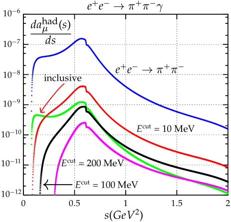
Figure 5: Differential contribution to $a_{\mu}^{\mathrm{had,\gamma}}$ from $\pi^{+}\pi^{-}\gamma$ intermediate states for different cutoff values compared with the complete contribution (virtual plus real corrections, labelled ‘inclusive’) evaluated in sQED (FSR), as well as with the contribution from the $\pi^{+}\pi^{-}$ intermediate state.

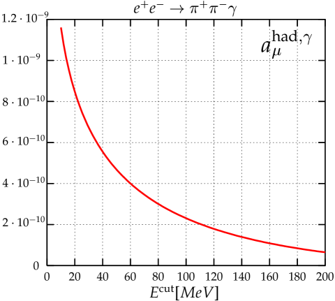
Figure 6: Integrated contribution to $a_{\mu}^{\mathrm{had,\gamma}}$ as a function of the cutoff $E^{\mathrm{cut}}$.

The strategy for the exclusive measurement now proceeds as follows:

The contribution from $R^{\mathrm{V+R}}(\pi^{+}\pi^{-}(\gamma),E^{\mathrm{cut}})$ as a function of $E^{\mathrm{cut}}$ can be measured by analysing final states where hard-photon radiation is suppressed by suitable chosen cuts on energy and collinearity of the pions. The $E^{\mathrm{cut}}$ dependence of $R^{\mathrm{H}}(\pi^{+}\pi^{-}\gamma,E^{\mathrm{cut}})$ can be measured by collecting $\pi^{+}\pi^{-}\gamma$ final states (and correcting of course for ISR) as discussed in Section 2. Alternatively we may correct for (unmeasured) hard photon events by employing a model like sQED, which has to be checked experimentally — at least for a few selected kinematic configurations.

Let us now estimate the contributions from hard photon radiation to $a_{\mu}$. In Fig. 5 we display the integrand

$$\frac{d}{ds}a^{\mathrm{had,\gamma}}_{\mu}(E^{\mathrm{cut}})=\frac{\alpha^{2}}{3\pi^{2}s}K(s)\ R^{\mathrm{H}}(s,E^{\mathrm{cut}})~{},$$ (8)

for $E^{\mathrm{cut}}=10$, $100$ and $200$ MeV as a function of $\sqrt{s}=m(\pi^{+}\pi^{-}\gamma)$ between the threshold and $2$ GeV. The result is compared with the complete sQED contribution, as derived from point-like pions, and the lowest order contribution from $\pi^{+}\pi^{-}$. The integrated result is displayed in Fig. 6.

Using sQED as a model, one finds that contributions from hard photon radiation, with a cut at $100$ MeV, are still small with respect to the present uncertainty $\delta a_{\mu}^{\mathrm{had,LO}}=7\times 10^{-10}$ Davier:2002dy ; HMNT02 . Let us emphasize that cuts on the photon energy around 50 MeV or below might well lead to important shifts in $a_{\mu}$. Of course we have assumed that hard radiation is not grossly underestimated by sQED, an assumption to be tested by experiment. As we will demonstrate in the next section, such tests are indeed feasible in experiments based on the radiative return.

4 FSR at next-to-leading order and the event generator PHOKHARA

As discussed in Section 2, the radiative return allows us to exploit the enormous luminosity of $\Phi$- and $B$-meson factories for the measurement of the hadronic cross section over a wide range of energies. On the basis of the leading order treatment, we have demonstrated that the analysis of final states with one photon allows us to determine the pion form factor for arbitrary $Q^{2}$ and the cross section for $\pi^{+}\pi^{-}$ plus a hard photon from FSR at $\sqrt{s}$.

Intuitively it should also be possible to exploit the radiative return for the extraction of FSR for arbitrary invariant mass $\sqrt{s^{\prime}}$ of the $\pi^{+}\pi^{-}\gamma$ system through the reaction

$$e^{+}e^{-}\to\gamma\gamma^{*}(\to\pi^{+}\pi^{-}\gamma)\ .$$ (9)

The implementation of this two-step process into PHOKHARA and the question of how to separate the corresponding amplitude from double photon emission from the initial or final state are the main topics of this section.

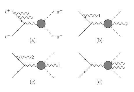
Figure 7: Typical amplitudes contributing to the reaction $e^{+}e^{-}\to\pi^{+}\pi^{-}\gamma\gamma$. For two photons emitted either from the electron/positron or the hadronic system. Only one representative is displayed.

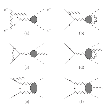
Figure 8: Typical amplitudes describing virtual corrections to the reaction $e^{+}e^{-}\to\pi^{+}\pi^{-}\gamma$. Permutations are omitted.

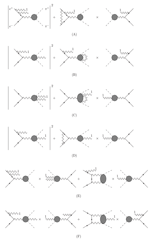
Figure 9: Charge-even infrared-finite combinations of amplitudes. The photon labelled ‘1’ is hard. Diagrams written in reverse order are to be understood as complex conjugate.

Let us first describe the main physics ingredients and assumptions of the new version of PHOKHARA (PHOKHARA 3.0). The complete set of diagrams relevant to the reaction

$$e^{+}e^{-}\to\pi^{+}\pi^{-}\gamma\gamma~{},$$ (10)

is displayed in Fig. 7. We require at least one photon (with four momentum $k_{1}$) to be hard, i.e. with energy $E_{1}>E_{\gamma}^{\mathrm{min}}$, where $E_{\gamma}^{\mathrm{min}}$ is typically around $5$ to $10$ MeV for DAΦNE energies and significantly larger (several GeV) for $B$-meson factories. We only display typical diagrams and omit permutations. However, we explicitly distinguish the two cases, where the hard photon is emitted either from the electron–positron line or from the hadronic system. Diagrams relevant to virtual corrections to the reaction with one photon,

$$e^{+}e^{-}\to\pi^{+}\pi^{-}\gamma~{},$$ (11)

are shown in Fig. 8; they contribute through their interference with the Born amplitude (Fig. 1). At this point no assumption about the form of the $\gamma^{*}\to\pi^{+}\pi^{-}\gamma$ coupling or the structure of the virtual corrections at the hadronic vertex is imposed.

Just as in leading order, charge-symmetric and asymmetric terms are present in the differential distribution. The latter are particularly sensitive to the FSR amplitude and may serve for tests of the FSR model or even for an independent determination of this amplitude for arbitrary $s^{\prime}$. In the present upgraded version of the program, only charge symmetric terms will be included, which are sufficient for the present purpose.

In Fig. 9 those combinations of (gauge-invariant sets of) amplitudes involving real and virtual radiation are displayed, which lead to infrared-finite charge-even combinations. The first (A) corresponds to the radiative corrections to the leptonic tensor, and has been derived in Rodrigo:2001jr ; Kuhn:2002xg . It is the crucial element of PHOKHARA (versions 1.0 and 2.0) and can be used for the simulation of arbitrary hadronic final states. The second combination (B) corresponds to the two-step process described in Eq. (9) above and is implemented in the present, newest version of PHOKHARA (version 3.0). Before discussing the actual implementation, let us discuss the remaining terms. The next combinations, denoted by (C) and (D), describe radiative corrections to pure FSR, with the leading process depicted in Fig. 1b. The hard photon originates from the hadronic system, and the radiative corrections (virtual, soft, and hard radiation) are either attached to the hadronic (C) or the leptonic (D) system. As discussed in Section 2, the leading order process can be controlled at DAΦNE through suitable cuts and FSR can be reduced to a level of less than 1%. At the energy of $10.52$ GeV, i.e. at $B$-meson factories, it is entirely irrelevant. Therefore we do not include these radiative corrections to an already small contribution in the program.

A similar argument applies to the remaining terms, denoted by (E) and (F). These describe radiative corrections (real and virtual photons) to the interference between hard ISR and hard FSR. They will be neglected on the basis of the same arguments as before.

In the following, we denote by ISRNLO the contributions to the cross section coming from ISR only calculated at NLO, i.e. those from Figs. 1a and 9A. IFSLO includes also the contribution from LO FSR (diagrams in Figs. 1a, 1b and 9A). Finally, IFSNLO includes on top of that initial plus final state emission at NLO (diagrams in Figs. 1a, 1b, 9A and 9B). Let us emphasize that these are gauge-invariant subsets throughout.

Let us now describe the implementation of the two-step process Eq. (9), denoted IFSNLO, in detail. Since we are only interested in final states with masses of the $\pi^{+}\pi^{-}\gamma$ system below $\approx$ 1 GeV, we expect sQED to provide a good description of the $\gamma^{*}\to\pi^{+}\pi^{-}\gamma$ amplitude. The virtual corrections are similarly modelled by sQED. They are combined with soft radiation, with $E_{2}<E_{2}^{\mathrm{cut}}$, to arrive at an infrared-finite result. The effective form factor is, therefore, introduced through the substitution

$$|F^{0}(Q^{2})|^{2} \to |F(Q^{2},E_{2}^{\mathrm{cut}})|^{2}=$$ (12)

$$|F^{0}(Q^{2})|^{2}\left(1+\frac{\alpha}{\pi}\eta^{\mathrm{V+S}}(Q^{2},E_{2}^{\mathrm{cut}})\right)\ ,\$$

with $\eta^{\mathrm{V+S}}(Q^{2},E_{2}^{\mathrm{cut}})$ given below. For the generation of real radiation the cutoff energy obviously refers to the $\pi^{+}\pi^{-}\gamma$ centre-of-mass frame.

It should be emphasized that only the combination $|F(Q^{2},E_{2}^{\mathrm{cut}})|^{2}$ is physically observable and relevant to the analysis of $a_{\mu}$ and $\alpha(m_{Z})$, of course after adding real radiation, which can either be measured, or for photon energies up to $\cal O$(100 MeV), modelled by sQED through the reaction

$$\kern-20.0pte^{+}(p_{1},\lambda_{e^{+}})\ +\ e^{-}(p_{2},\lambda_{e^{-}})\to$$

$$\kern 10.0pt\pi^{+}(q_{1})\ +\ \pi^{-}(q_{2})\ +\ \gamma(k_{1},\lambda_{1})\ +\ \gamma(k_{2},\lambda_{2})~{}.$$

(13)

The helicity amplitudes responsible for real radiation (Fig. 7b and c) are given by the sum of 12 Feynman amplitudes. Adopting a notation similar to Rodrigo:2001kf , they read

$$M^{\mathrm{H}}_{\mathrm{IFSNLO}}(\lambda_{e^{+}},\lambda_{e^{-}},\lambda_{1},\lambda_{2})=-\frac{(4\pi\alpha)^{2}}{\hat{Q}^{2}}\biggl{\{}$$

$$v_{I}^{\dagger}(p_{1},\lambda_{e^{+}})\ A\ u_{I}(p_{2},\lambda_{e^{-}})+v_{II}^{\dagger}(p_{1},\lambda_{e^{+}})\ B\ u_{II}(p_{2},\lambda_{e^{-}})\biggl{\}}$$

$$+\ \ \ \bigl{(}k_{1}\leftrightarrow k_{2}\bigr{)}\ \ \ ,$$ (14)

where the index H indicates that both photons are hard, and

$$A =\frac{\left(\varepsilon^{*}(k_{1},\lambda_{1})^{-}k_{1}^{+}-2\varepsilon^{*}(k_{1},\lambda_{1})\cdot p_{1}\right)J^{-}}{2k_{1}\cdot p_{1}}$$

$$+\frac{J^{-}\left(2\varepsilon^{*}(k_{1},\lambda_{1})\cdot p_{2}-k_{1}^{+}\varepsilon^{*}(k_{1},\lambda_{1})^{-}\right)}{2k_{1}\cdot p_{2}}~{},$$ (15)

$$B =\frac{\left(\varepsilon^{*}(k_{1},\lambda_{1})^{+}k_{1}^{-}-2\varepsilon^{*}(k_{1},\lambda_{1})\cdot p_{1}\right)J^{+}}{2k_{1}\cdot p_{1}}$$

$$+\frac{J^{+}\left(2\varepsilon^{*}(k_{1},\lambda_{1})\cdot p_{2}-k_{1}^{-}\varepsilon^{*}(k_{1},\lambda_{1})^{+}\right)}{2k_{1}\cdot p_{2}}~{},$$ (16)

with

$$\hat{Q}=p_{1}+p_{2}-k_{1}=q_{1}+q_{2}+k_{2}~{},\qquad s^{\prime}=\hat{Q}^{2}~{},$$ (17)

and $J^{\mu}$ being the current describing the $\pi^{+}\pi^{-}\gamma$ final state

$$J^{\mu}=iF_{2\pi}(s^{\prime})\ D^{\mu}~{},$$ (18)

where

$$D^{\mu}=\left(q_{1}+k_{2}-q_{2}\right)^{\mu}\frac{q_{1}\cdot\varepsilon^{*}(k_{2},\lambda_{2})}{q_{1}\cdot k_{2}}$$

$$+\left(q_{2}+k_{2}-q_{1}\right)^{\mu}\frac{q_{2}\cdot\varepsilon^{*}(k_{2},\lambda_{2})}{q_{2}\cdot k_{2}}-2\varepsilon^{*\mu}(k_{2},\lambda_{2})\ ,$$ (19)

and $k^{\pm},J^{\pm}$ are 2$\times$2 matrices, which can be found in Rodrigo:2001kf . We do not include contributions from the radiative decay $\phi\to\pi^{+}\pi^{-}\gamma$. Their effect is small, can be well controlled and was discussed in Melnikov:2000gs .

In the present version of the program, one of the photons is assumed to be visible, at least in principle, and only the photon emitted from final states is allowed to be soft (Fig. 9B). For photon energies $w\sqrt{s}<E_{1\gamma}<E_{c}^{v}$ (or $w\sqrt{s}<E_{2\gamma}<E_{c}^{v}$) the amplitude used consists of 6 diagrams only. $E_{c}^{v}$ is the threshold above which we can ‘observe’ the photon — typically $10$ MeV for DAΦNE and 100 MeV for $B$-factories. If both photons are hard, $E_{1\gamma},~{}E_{2\gamma}>E_{c}^{v}$ the sum of 12 diagrams is used.

The corresponding virtual plus soft photon corrections can be written as

$$d\sigma^{\mathrm{V+S}}_{\mathrm{IFSNLO}}=\frac{\alpha}{\pi}\ \eta^{\mathrm{V+S}}(s^{\prime},E_{2}^{\mathrm{cut}})\ d\sigma^{(0)}_{\mathrm{ISR}}(s^{\prime})~{},$$ (20)

where $d\sigma^{(0)}_{\mathrm{ISR}}$ is the leading order $e^{+}e^{-}\to\pi^{+}\pi^{-}\gamma$ cross section, with the photon emitted off the initial leptons only, and

$$\eta^{\mathrm{V+S}}(s^{\prime},E_{2}^{\mathrm{cut}})=-2\biggl{[}\frac{1+\beta^{2}}{2\beta}\log(t)+1\biggr{]}\log(2w)$$

$$-\frac{2+\beta^{2}}{\beta}\log(t)-2+\log\biggl{(}\frac{1-\beta^{2}}{4}\biggr{)}$$

$$-\frac{1+\beta^{2}}{2\beta}\biggl{\{}-\log(t)\log\biggl{(}\frac{\beta(1+\beta)}{2}\biggr{)}$$

$$+\log\biggl{(}\frac{1+\beta}{2\beta}\biggr{)}\log\biggl{(}\frac{1-\beta}{2\beta}\biggr{)}$$

$$+2\hbox{Li}_{2}\biggl{(}\frac{2\beta}{1+\beta}\biggr{)}+2\hbox{Li}_{2}\biggl{(}-\frac{1-\beta}{2\beta}\biggr{)}-\frac{2}{3}\pi^{2}\biggr{\}}~{},$$

where $w=E_{2}^{\mathrm{cut}}/\sqrt{s^{\prime}}$, and

$$\beta=\sqrt{1-4m_{\pi}^{2}/s^{\prime}}~{},\qquad t=\frac{1-\beta}{1+\beta}~{}.$$ (22)

The function $\eta^{\mathrm{V+S}}(s^{\prime},E_{2}^{\mathrm{cut}})$ is of course the familiar correction factor derived in Schwinger:ix for the reaction $e^{+}e^{-}\to\pi^{+}\pi^{-}\gamma$ in the framework of sQED (see also Gluza:eta ). For the present case, $s^{\prime}$ corresponds to the squared mass of the $\pi^{+}\pi^{-}\gamma$ system, and for virtual and soft photon emission, $s^{\prime}\simeq Q^{2}$, the soft photon cutoff is defined in the $\pi^{+}\pi^{-}\gamma$ rest frame.

Correspondingly the cross section for the reaction

$$e^{+}e^{-}\to\gamma(k_{1})\gamma^{*}(\to\pi^{+}\pi^{-}\gamma(k_{2}))~{},$$ (23)

after integration over the angles and energy (from $E_{2}^{\mathrm{cut}}$ to the kinematical limit) of $\gamma(k_{2})$ , is given by

$$d\sigma^{\mathrm{H}}_{\mathrm{IFSNLO}}=\frac{\alpha}{\pi}\ \eta^{\mathrm{H}}(s^{\prime},E_{2}^{\mathrm{cut}})\ d\sigma^{(0)}_{\mathrm{ISR}}(s^{\prime})~{},$$ (24)

with

$$\eta^{\mathrm{H}}(s^{\prime},E_{2}^{\mathrm{cut}})=-\frac{1+\beta^{2}}{\beta}\biggl{[}\hbox{Li}_{2}\biggl{(}1-\frac{t_{m}}{t}\biggr{)}-\hbox{Li}_{2}(t_{m}t)$$

$$+\zeta(2)+\frac{\log^{2}(t)}{2}\biggr{]}-\log(t_{m}-t)\biggl{[}\frac{1+\beta^{2}}{\beta}\log\biggl{(}\frac{t_{m}}{t}\biggr{)}$$

$$-2\biggr{]}-\frac{(1-\beta^{2})\beta_{m}}{2\beta^{3}(1-\beta_{m}^{2})}\biggl{[}\frac{2(1-\beta^{2})}{1-\beta_{m}^{2}}-7\beta^{2}-5\biggr{]}$$

$$+\frac{\log(t_{m})}{\beta}\biggl{\{}-2+\frac{1-\beta^{2}}{4}\biggl{[}1+\frac{8}{1-\beta_{m}^{2}}+\frac{3}{\beta^{2}}\biggr{]}$$

$$+(1+\beta^{2})\biggl{[}\log\biggl{(}\frac{4(\beta^{2}-\beta_{m}^{2})}{(1+\beta)^{2}(1-\beta_{m}^{2})}\biggr{)}+\frac{\log(t_{m})}{2}\biggr{]}\biggr{\}}$$

$$-2\log(1-t_{m}t)~{},$$ (25)

where $t$ and $\beta$ are defined in Eq. (22), and

$$\beta_{m}\equiv\sqrt{1-\frac{4m^{2}_{\pi}}{Q_{m}^{2}}}~{},\qquad t_{m}=\frac{1-\beta_{m}}{1+\beta_{m}}~{}.$$

Here $Q_{m}^{2}$ is the maximum value of $Q^{2}$

$$Q_{m}^{2}=s^{\prime}-2E_{2}^{\mathrm{cut}}\sqrt{s^{\prime}}~{},$$

and $E_{2}^{\mathrm{cut}}$ is again defined in the $\gamma^{*}$ rest frame. This formula will be useful for tests of the Monte Carlo event generator discussed below, and $E_{2}^{\mathrm{cut}}$ is still arbitrary at this point. The same formula can also be used to test FSR at LO with $s^{\prime}\to s$ and $E_{2}^{\mathrm{cut}}$ set now in the $e^{+}e^{-}$ cms frame.

For $E_{2}^{\mathrm{cut}}$ small, $w=E_{2}^{\mathrm{cut}}/\sqrt{s^{\prime}}\ll 1$, the function $\eta^{\mathrm{H}}$ reduces to

$$\kern-5.0pt\eta^{\mathrm{H}}(s^{\prime},E_{2}^{\mathrm{cut}})\simeq\log(2w)\biggl{[}2+\frac{1+\beta^{2}}{\beta}\log(t)\biggr{]}$$ (26)

$$\kern-5.0pt-\frac{(1+\beta^{2})}{\beta}\biggl{[}\log(t^{2})\log(1-t)+\hbox{Li}_{2}(1-t^{2})\biggr{]}$$

$$\kern-5.0pt+\frac{(1-\beta^{2})(3+\beta^{2})}{4\beta^{3}}\log(t)+2\log\biggl{(}\frac{1-\beta^{2}}{4\beta^{2}}\biggr{)}+\frac{3}{2\beta^{2}}+\frac{7}{2}~{}.$$

Adding virtual, soft (Eq. (LABEL:etavs)) and hard (Eq. (26)) corrections, the familiar correction factor Schwinger:ix ; Drees:1990te ; Melnikov:2001uw

$$\eta(s^{\prime})=\frac{1+\beta^{2}}{\beta}\biggl{\{}4\hbox{Li}_{2}\biggl{(}\frac{1-\beta}{1+\beta}\biggr{)}+2\hbox{Li}_{2}\biggl{(}-\frac{1-\beta}{1+\beta}\biggr{)}$$

$$-3\log\biggl{(}\frac{2}{1+\beta}\biggr{)}\log\biggl{(}\frac{1+\beta}{1-\beta}\biggr{)}-2\log(\beta)\log\biggl{(}\frac{1+\beta}{1-\beta}\biggr{)}\biggr{\}}$$

$$+\frac{1}{\beta^{3}}\biggl{[}\frac{5}{4}(1+\beta^{2})^{2}-2\biggr{]}\log\biggl{(}\frac{1+\beta}{1-\beta}\biggr{)}+3\log\biggl{(}\frac{1-\beta^{2}}{4}\biggr{)}$$

$$-4\log(\beta)+\frac{3~{}(1+\beta^{2})}{2\beta^{2}}~{},$$ (27)

is recovered.

Using Eqs. (LABEL:etavs) and (25) the implementation of FSR in combination with ISR is straightforward. To match hard, soft and virtual radiation smoothly, the energy cutoff ($E_{2}^{\mathrm{cut}}$) has to be transformed from the rest frame of the $\pi^{+}\pi^{-}\gamma$ (emitted from the final state) system to the laboratory frame ($e^{+}e^{-}$ cms frame) ($E_{\gamma}^{\mathrm{min}}$). In fact it is necessary to recalculate the soft photon contribution, as the cut on $Q^{2}$ depends in the latter case on the angle between the two emitted photons and now

$$\eta^{\mathrm{V+S}}(s,s^{\prime},E_{\gamma}^{\mathrm{min}})=-2\biggl{[}\frac{1+\beta^{2}}{2\beta}\log(t)+1\biggr{]}$$

$$\times\biggl{[}\log(2w)+1+\frac{s^{\prime}}{s^{\prime}-s}\log\biggl{(}\frac{s}{s^{\prime}}\biggr{)}\biggr{]}$$

$$-\frac{2+\beta^{2}}{\beta}\log(t)-2+\log\biggl{(}\frac{1-\beta^{2}}{4}\biggr{)}$$

$$-\frac{1+\beta^{2}}{2\beta}\biggl{\{}-\log(t)\log\biggl{(}\frac{\beta(1+\beta)}{2}\biggr{)}$$

$$+\log\biggl{(}\frac{1+\beta}{2\beta}\biggr{)}\log\biggl{(}\frac{1-\beta}{2\beta}\biggr{)}$$

$$+2\hbox{Li}_{2}\biggl{(}\frac{2\beta}{1+\beta}\biggr{)}+2\hbox{Li}_{2}\biggl{(}-\frac{1-\beta}{2\beta}\biggr{)}-\frac{2}{3}\pi^{2}\biggr{\}}~{},$$ (28)

where $\beta$ is defined in Eq. (22) and $w=E_{\gamma}^{\mathrm{min}}/\sqrt{s}$ .

Table 1: Total cross section (nb) for the process $e^{+}e^{-}\rightarrow\pi^{+}\pi^{-}\gamma(\gamma)$ for different values of the soft photon cutoff. One of the photons is required to have an energy larger than 10 MeV (100 MeV) for $\sqrt{s}=1.02$ GeV (10.52 GeV). No further cuts applied in columns 2 and 3. In column 4, the pion angles are restricted to $40^{\circ}<\theta_{\pi^{\pm}}<140^{\circ}$ and the photon(s) angles to $\theta_{\gamma}<15^{\circ}$ or $\theta_{\gamma}>165^{\circ}$.

$w$	$\sqrt{s}=$1.02 GeV	10.52 GeV	1.02 GeV
$10^{-3}$	40.992 (5)	0.1606 (1)	20.988 (1)
$10^{-4}$	41.013 (6)	0.1607 (2)	20.993 (1)
$10^{-5}$	41.018 (7)	0.1607 (2)	20.995 (2)

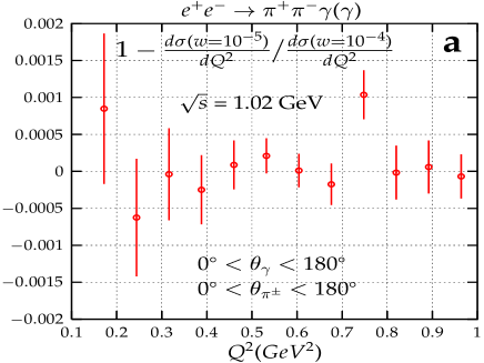
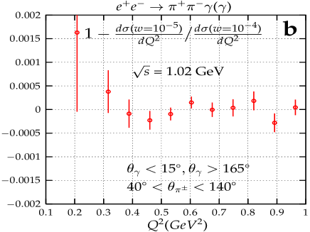
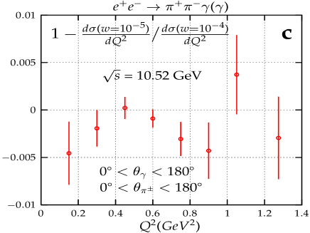
Figure 10: Comparison of the $Q^{2}$ distribution for two values of the soft photon cutoff ($w=10^{-4}$ vs. $10^{-5}$) for $\sqrt{s}=1.02$ GeV (a,b) and $\sqrt{s}=10.52$ GeV (c). One of the photons was required to have energy $>$ 10 MeV (for $\sqrt{s}=1.02$ GeV) and $>$ 100 MeV (for $\sqrt{s}=10.52$ GeV). Angular cuts were applied only on plot (b), where pion polar angles are restricted to $40^{\circ}<\theta_{\pi^{\pm}}<140^{\circ}$ and photon polar angles to $\theta_{\gamma}<15^{\circ}$ and $\theta_{\gamma}>165^{\circ}$.

A number of tests were performed to ensure the technical precision of the new version of PHOKHARA. The square of the matrix element summed over polarizations of the final particles and averaged over polarizations of the initial particles was calculated with FORM FORM using the standard trace method. External gauge invariance was checked analytically when using the trace method and numerically for the amplitude calculated with the helicity amplitude method. The two results for the square of the matrix element summed over polarizations, were compared numerically. The code based on the result from the trace method was written in quadrupole precision to reduce cancellations. The code based on the result obtained with the helicity amplitude method, uses double-precision for real and complex numbers and is now incorporated in the code of PHOKHARA 3.0. Agreement of 13 significant digits (or better) was found between both codes. The sensitivity of the integrated cross section — with and without angular cuts — to the choice of the cutoff $w$ can be deduced from Table 1 and Fig. 10. For simplicity the same separation parameter $w$ was chosen for ISR and FSR corrections. Choosing $w=10^{-4}$ or less, the result becomes independent of $w$. The tests prove that the analytical formula describing soft photon emission as well as the Monte Carlo integration in the soft photon region are well implemented in the program. Having analytical expressions for $\eta^{\mathrm{H}}(s,E_{\gamma}^{\mathrm{min}})$ (Eq. (25)) we can test also the implementation of hard photon emission from the final state. The results of the tests are collected in Figs. 11 and 12, where FSR at LO obtained from PHOKHARA is compared with the analytical result for the corresponding cross section:

$$\sigma_{\mathrm{FSR}}(s) =\frac{\alpha}{\pi}\ \eta^{\mathrm{H}}(s,E_{\gamma}^{\mathrm{min}})\ \sigma_{0}(s)$$

$$=\frac{\alpha}{\pi}\ \eta^{\mathrm{H}}(s,E_{\gamma}^{\mathrm{min}})\ \frac{\pi}{3}\frac{\alpha^{2}\beta^{3}(s)}{s}\mid F_{2\pi}(s)\mid^{2}~{},$$ (29)

for a fixed value of the photon energy cutoff and different values of the $e^{+}e^{-}$ cms energy (Fig. 11) or fixed value of the $e^{+}e^{-}$ cms energy and various values of the photon energy cutoff (Fig. 12). As one can see the technical precision of that part of PHOKHARA is much better than 1 per mille. The IFSNLO part was also tested against the analytical result

$$\eta(s^{\prime})=\frac{d\sigma^{\mathrm{V+S+H}}_{\mathrm{IFSNLO}}(s,s^{\prime})/ds^{\prime}}{\frac{\alpha}{\pi}\ d\sigma^{(0)}_{\mathrm{ISR}}(s^{\prime})/ds^{\prime}}\ .$$ (30)

The results of the tests are shown in Fig. 13. The agreement of $\eta$ calculated by PHOKHARA and the analytical result (Eq. (27)) is at the level of a few per mille. However, since the contribution to the cross section of that part is multiplied by $\alpha/\pi\simeq 1/400$, the actual technical precision of the IFSNLO PHOKHARA cross section is at the level of $10^{-5}$.

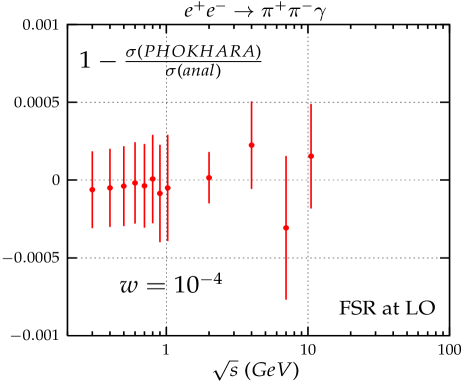
Figure 11: Comparison between the LO FSR cross section calculated analytically (Eq. (29)) and calculated by PHOKHARA for fixed value of $w=E_{\gamma}^{\mathrm{min}}/\sqrt{s}$.

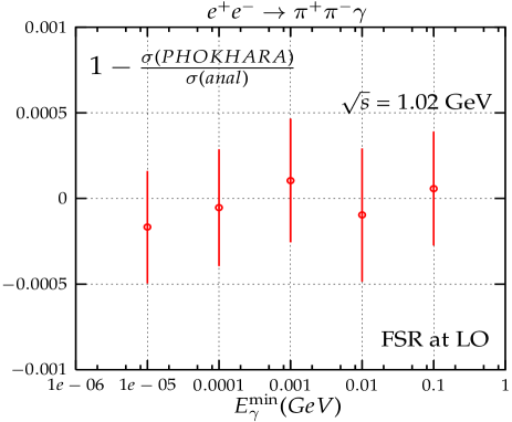
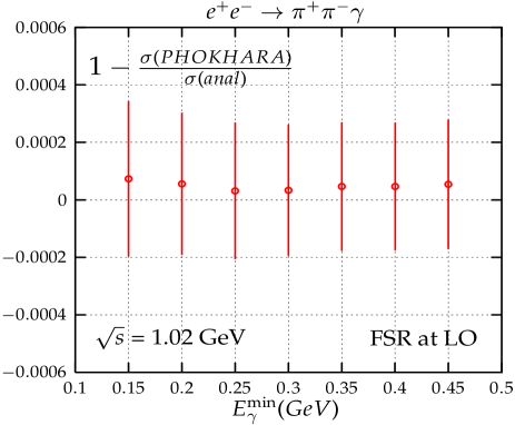
Figure 12: Comparison between the LO FSR cross section calculated analytically (Eq. (29)) and calculated by PHOKHARA for a fixed value of $\sqrt{s}=1.02$ GeV.

5 FSR contribution to the hadronic cross section and its measurement via the radiative return method

We shall study now the impact of the new corrections on various distributions. Before entering the discussion, let us recall the meaning of various abbreviations, which will be used in the following. ISRNLO corresponds to the ISR cross section calculated at NLO without any FSR. IFSLO includes in addition FSR at LO. Finally, IFSNLO stands for ISR and FSR at NLO as implemented in the new version of PHOKHARA (version 3.0).

Let us start the discussion for a cms energy of 1.02 GeV, relevant for the KLOE experiment. The IFSNLO correction to the cross section from graphs in Fig. 9B is relatively big at low $Q^{2}$, if no cuts are applied (Fig. 14a). Below the $\rho$ resonance, they grow from zero at the resonance to 10% of the IFSLO cross section near the production threshold, while they remain small above the $\rho$ resonance. This is due to the fact that the ISR leading to the $\rho$ meson is strongly enhanced. Subsequently the $\rho$ decays into $\pi^{+}\pi^{-}\gamma$, with a large contribution from the region where $Q^{2}$, the invariant mass of the $\pi^{+}\pi^{-}$, is low. Of course this is smeared by the width of the $\rho$, but the above discussion remains valid and the contribution from the newly implemented diagrams, through the reaction $e^{+}e^{-}\to\gamma\rho(\to\gamma\pi^{+}\pi^{-})$, is sizeable.

The effect of several ‘standard cuts’ at $\sqrt{s}=1.02$ GeV is shown in Figs. 14b and 14c. The sensitivity of the newly implemented contributions to these cuts can be exploited to test, control or experimentally eliminate FSR at NLO. It is relatively easy to find cuts that lower the correction to a level of 2%–3%. In fact all the cuts which were used to eliminate FSR at LO are also effective here. The standard KLOE cut on the track mass Achim:radcor02 reduces FSR further, to less than 1% for most of the $Q^{2}$ range, apart of the high values of $Q^{2}$, where the corrections remain at the level of 2%-3% (Fig. 14c, lower curve).

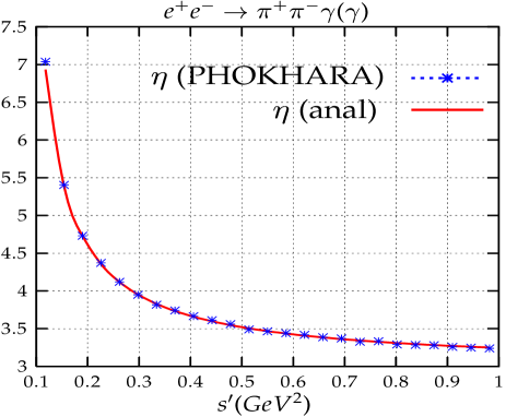
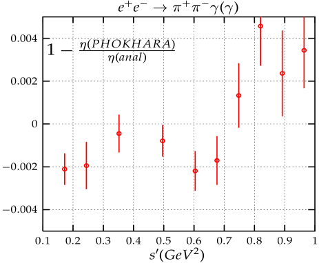
Figure 13: Comparison between the function $\eta$ obtained from Eq.(27) and from PHOKHARA.

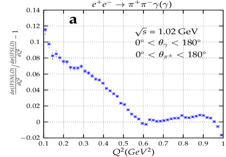
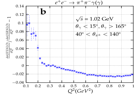
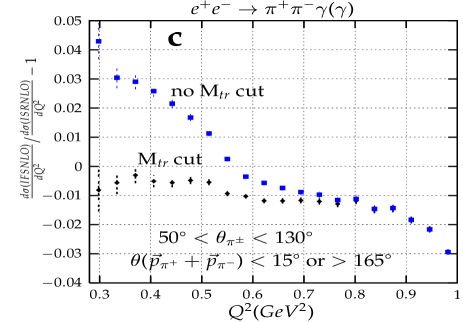
Figure 14: Comparison of the $Q^{2}$ differential cross sections for $\sqrt{s}=1.02$  GeV: IFSNLO contains the complete NLO contribution, while IFSLO has FSR only at LO. The pion and photon(s) angles are not restricted in (a), and restricted in (b). In (c) the cuts are imposed on the missing momentum direction and the track mass (see text for description).

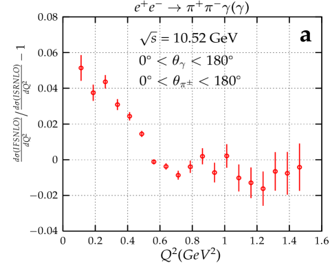
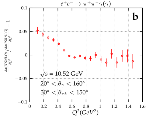
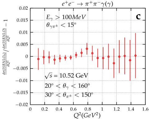
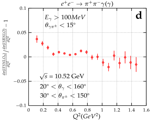
Figure 15: Comparisons of IFSNLO and ISRNLO distributions without (a) and with (b) angular cuts and the effect of the ‘reassigning’ (samples labelled $rs$) process described in the text on the data samples generated in ISRNLO (c) and IFSNLO (d).

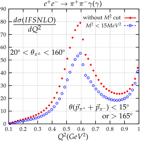
Figure 16: Dependence of the IFSNLO differential cross section on the cut on missing invariant mass $M^{2}$.

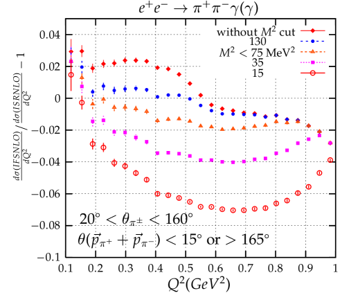
Figure 17: Dependence of the relative IFSNLO contribution on the cut on missing invariant mass $M^{2}$.

The behaviour of the additional contribution at 10.52 GeV is qualitatively similar. Without cuts the relative enhancement amounts to approximately 4% (Fig. 15a), and this remains unchanged after cuts on pion and photon angles, which correspond to the detector acceptance, are introduced (Fig. 15b). As stated before, a large fraction of the excess is due to the feed-down from the $\rho$-meson in the two step process $e^{+}e^{-}\to\gamma\rho(\to\pi^{+}\pi^{-}\gamma)$. Assuming, that hard photons, say above 100 MeV, can be identified, we try to identify these events by assigning photons with small angles relative to $\pi^{+}$ or $\pi^{-}$ (say 15^∘) to the hadronic system when $M_{\rho}-\Gamma_{\rho}<\sqrt{(p_{+}+p_{-}+p_{\gamma})^{2}}<M_{\rho}+\Gamma_{\rho}$, thus moving these events from $Q^{2}=(p_{+}+p_{-})^{2}$ to $Q^{2}=(p_{+}+p_{-}+p_{\gamma})^{2}$. For a sample generated with PHOKHARA 3.0 without FSR at NLO the distribution remains practically the same (Fig. 15c), while including FSR at NLO the excess in the low $Q^{2}$ region is significantly reduced (Fig. 15d). In fact, part of the remaining enhancement (about 1 to 2% for $Q^{2}$ between 0.2 and 0.1 GeV² ) just corresponds to the effect of multiplication with the factor $\frac{\alpha}{\pi}\eta(s^{\prime})$.

The FSR corrections originating from the ‘two–step’ process and their effect on cuts necessarily introduce some model dependence into the extraction of the pion form factor. The detection and analysis of the complete final state — charged pions as well as photons — is of course optimal for the study of this phenomena. However, the present KLOE analysis is based on the measurement of the $\pi^{+}$ and $\pi^{-}$ momenta only. Even this partial information allows to construct distributions, which are sensitive to final states with $\pi^{+}$ $\pi^{-}$ and two photons. As an alternative to the straightforward study of the $Q^{2}$ distribution and its Monte Carlo simulation it is thus even possible to test the model governing the production of $\pi^{+}\pi^{-}$ in conjunction with two photons and constrain or even measure the process $\gamma^{*}\to\pi^{+}\pi^{-}(\gamma)$, an important ingredient for the precise prediction of $a_{\mu}^{\mathrm{had,LO}}$.

The response of $d\sigma_{\mathrm{IFSNLO}}/dQ^{2}$ to different cuts on $M^{2}$, the invariant mass of the recoiling photonic system (Fig. 16) will be an important observable. Contributions with double emission from the initial state and from mixed ISR–FSR will be affected by this cut. However, the cut dependence is markedly different for $d\sigma_{\mathrm{IFSNLO}}/dQ^{2}$ (which includes both contributions) and $d\sigma_{\mathrm{ISRNLO}}/dQ^{2}$ (which includes configurations from ISR only) as shown in Fig. 17. The confirmation of the $M^{2}$ dependence as predicted by PHOKHARA, as well as the verification of charge asymmetric distributions (see Section 2) would provide additional support for the ansatz of emission from point-like pions or allow to test alternative models.

6 Conclusions

Measurements of the pion form factor through the radiative return offer the unique possibility for improved predictions for the muon magnetic moment and the electromagnetic coupling $\alpha(M_{Z})$. Contributions to the dispersion integral from intermediate states with $\pi^{+}\pi^{-}$ and a photon start to become relevant at the present level of precision and can be measured in reactions leading to $\pi^{+}\pi^{-}$ in conjunction with two photons. An upgraded version of PHOKHARA (version 3.0), which includes simultaneous emission of photons from the initial and the final state, has been presented. The two step process $e^{+}e^{-}\to\gamma\rho(\to\pi^{+}\pi^{-}\gamma)$ leads to a notable enhancement of events with low mass of the $\pi^{+}\pi^{-}$ system. Various cuts are described, which allow to control this effect, to identify these events, correct the distribution and test the model for final state radiation.

References

- (1) K. G. Chetyrkin, J. H. Kühn and A. Kwiatkowski, Phys. Rep. 277 (1996) 189.
- (2) R. V. Harlander and M. Steinhauser, Comput. Phys. Commun. 153 (2003) 244 [hep-ph/0212294].
- (3) ALEPH, DELPHI, L3 and OPAL Collaborations, LEP Electroweak Working Group and SLD Heavy Flavor and Electroweak Groups (D. Abbaneo et al.) [hep-ex/0112021].
- (4) J. H. Kühn and M. Steinhauser, Nucl. Phys. B619 (2001) 588 [hep-ph/0109084].
- (5) S. Eidelman and F. Jegerlehner, Z. Phys. C67 (1995) 585 [hep-ph/9502298].
- (6) F. Jegerlehner, J. Phys. G29 (2003)101 [hep-ph/0104304].
- (7) K. Melnikov, Int. J. Mod. Phys. A 16 (2001) 4591 [hep-ph/0105267].
- (8) M. Davier, S. Eidelman, A. Höcker and Z. Zhang, hep-ph/0308213.
- (9) K. Hagiwara, A.D. Martin, Daisuke Nomura and T. Teubner, Phys. Lett. B 557 (2003) 69 [hep-ph/0209187].
- (10) G.W.Bennett et al. [Muon Collaboration], Phys. Rev. Lett. 89 (2002) 101804; Erratum, ibid. 89 (2002) 129903, [hep-ex/0208001].
- (11) S. Binner, J. H. Kühn and K. Melnikov, Phys. Lett. B 459 (1999) 279 [hep-ph/9902399].
- (12) Min-Shih Chen and P. M. Zerwas, Phys. Rev. D 11 (1975) 58.
- (13) H. Czyż and J. H. Kühn, Eur. Phys. J. C 18 (2001) 497 [hep-ph/0008262].
- (14) G. Rodrigo, A. Gehrmann-De Ridder, M. Guilleaume and J. H. Kühn, Eur. Phys. J. C 22 (2001) 81 [hep-ph/0106132].
- (15) G. Rodrigo, Acta Phys. Polon. B 32 (2001) 3833 [hep-ph/0111151].
- (16) G. Rodrigo, H. Czyż, J.H. Kühn and M. Szopa, Eur. Phys. J. C 24 (2002) 71 [hep-ph/0112184].
- (17) J. H. Kühn and G. Rodrigo, Eur. Phys. J. C 25 (2002) 215 [hep-ph/0204283].
- (18) H. Czyż, A. Grzelińska, J. H. Kühn and G. Rodrigo, Eur. Phys. J. C 27 (2003) 563 [hep-ph/0212225].
- (19) J. H. Kühn, Nucl. Phys. Proc. Suppl. 98 (2001) 289 [hep-ph/0101100].
- (20) G. Rodrigo, H. Czyż and J. H. Kühn, hep-ph/0205097; Nucl. Phys. Proc. Suppl. 123 (2003) 167 [hep-ph/0210287]; Nucl. Phys. Proc. Suppl. 116 (2003) 249 [hep-ph/0211186].
- (21) G. Cataldi, A. Denig, W. Kluge, S. Muller and G. Venanzoni, Frascati Physics Series (2000) 569.
- (22) M. Adinolfi et al. [KLOE Collaboration], hep-ex/0006036.
- (23) A. Aloisio et al. [KLOE Collaboration], hep-ex/0107023.
- (24) A. Denig et al. [KLOE Collaboration], eConf C010430 (2001) T07 [hep-ex/0106100].
- (25) E. P. Solodov [BABAR collaboration], eConf C010430 (2001) T03 [hep-ex/0107027].
- (26) B. Valeriani et al. [KLOE Collaboration], hep-ex/0205046.
- (27) N. Berger, eConf C020620 (2002) THAP10 [hep-ex/0209062].
- (28) G. Venanzoni et al. [KLOE Collaboration], eConf C0209101 (2002) WE07 [hep-ex/0210013]; hep-ex/0211005.
- (29) A. Denig et al. [KLOE Collaboration], Nucl. Phys. Proc. Suppl. 116 (2003)243 [hep-ex/0211024].
- (30) A. Aloisio et al. [KLOE Collaboration], hep-ex/0307051.
- (31) A. Blinov, talk at International Conference ‘New Trends in High-energy Physics’ Alushta, Crimea (May 2003) http://www.slac.stanford.edu/ ablinov/
- (32) J. Lee-Franzini, talk at Lepton Int. Sym. 2003, http://g2pc1.bu.edu/leptonmom/
- (33) J. Gluza, A. Hoefer, S. Jadach and F. Jegerlehner, Eur. Phys. J. C28 (2003) 261, [hep-ph/0212386] .
- (34) S. Groote, J.G. Körner and A.A. Pivovarov, Eur. Phys. J. C24 (2002) 393 [hep-ph/0111206].
- (35) R.R. Akhmetshin et al., Phys. Lett. B 527 (2002) 161 [hep-ex/0112031].
- (36) K. Melnikov, F. Nguyen, B. Valeriani and G. Venanzoni, Phys. Lett. B477 (2000) 114 [hep-ph/0001064].
- (37) J. S. Schwinger, Particles, Sources, and Fields. Vol. 3, Redwood City, USA: Addison-Wesley (1989) p. 99.
- (38) A. Hoefer, J. Gluza and F. Jegerlehner, Eur. Phys. J. C24 (2002) 51 [hep-ph/0107154].
- (39) M. Drees and K. i. Hikasa, Phys. Lett. B 252 (1990) 127.
- (40) J. A. M. Vermaseren, Symbolic Manipulations with FORM, Computer Algebra Nederland, Amsterdam, 1991.