Factorization fits and the unitarity triangle in charmless two-body $B$ decays

Abstract

We present fits to charmless hadronic $B$ decay data from the BaBar, Belle and Cleo experiments using two theoretical models: (i) the QCD factorization model of Beneke et al. and (ii) QCD factorization complemented with the so-called charming penguins of Ciuchini et al. When we include the data from pseudoscalar-vector decays the results favor the incorporation of the charming penguin terms. We also present fit results for the unitarity triangle parameters and the CP-violating asymmetries.

I Introduction

A wealth of experimental data on hadronic charmless $B$ decays has become available from the BaBar and Belle experiments. These studies of the numerous $B$ decay channels are designed to test the Cabbibo-Kobayashi-Maskawa (CKM) explanation of $CP$ violation in the standard model as represented by the unitarity triangle condition $V_{ud}V^{*}_{ub}+V_{cd}V^{*}_{cb}+V_{td}V^{*}_{tb}=0$ on the CKM mixing parameters. Such tests have been facilitated by the recent significant progress in the theoretical understanding of hadronic decay amplitudes based upon QCD factorization which allows the amplitudes to be expressed in terms of numerous soft QCD parameters, such as meson decay constants and transition form factors, and a set of calculable coefficients. In this paper we present an analysis of recent data, based upon QCD factorization. We also investigate the potential contribution to the decay amplitudes of $b$ quark annihilation and so-called charming penguins. The data that we attempt to fit includes decays to pseudoscalar ($\pi$ and $K$) and vector ($\rho,\omega,K^{*}$ and $\phi$) mesons. This is an extension of an earlier study Cott that was based upon simplified formulae derived from the heavy quark limit of QCD factorization.

The starting point for the calculation of all $B$ meson decay amplitudes is the effective Hamiltonian

$$\mathcal{H}_{\text{eff}}(\mu)=\frac{G_{F}}{\sqrt{2}}\sum_{p=u,c}\lambda_{p}[C_{1}(\mu)Q^{p}_{1}+C_{2}(\mu)Q^{p}_{2}+\sum_{i=3,\ldots,10}C_{i}(\mu)Q_{i}]+\text{other terms}$$ (1)

where $\lambda_{p}=V^{*}_{pq}V_{pb}$ is a product of CKM matrix elements, $q=d,s$ and the local $\Delta B=1$ four-quark operators are

$$Q^{p}_{1} = (\bar{q}_{\alpha}p_{\alpha})_{V-A}(\bar{p}_{\beta}b_{\beta})_{V-A},$$

$$Q^{p}_{2} = (\bar{q}_{\alpha}p_{\beta})_{V-A}(\bar{p}_{\beta}b_{\alpha})_{V-A},$$

$$Q_{3,5} = (\bar{q}_{\beta}b_{\beta})_{V-A}\sum_{q^{\prime}}(\bar{q}^{\prime}_{\alpha}q^{\prime}_{\alpha})_{V\mp A},$$

$$Q_{4,6} = (\bar{q}_{\beta}b_{\alpha})_{V-A}\sum_{q^{\prime}}(\bar{q}^{\prime}_{\alpha}q^{\prime}_{\beta})_{V\mp A},$$

$$Q_{7,9} = (\bar{q}_{\beta}b_{\beta})_{V-A}\sum_{q^{\prime}}(\bar{q}^{\prime}_{\alpha}q^{\prime}_{\alpha})_{V\pm A},$$

$$Q_{8,10} = (\bar{q}_{\beta}b_{\alpha})_{V-A}\sum_{q^{\prime}}(\bar{q}^{\prime}_{\alpha}q^{\prime}_{\beta})_{V\pm A},$$ (2)

where $q^{\prime}\in\{u,d,s,c\}$, $\alpha$ and $\beta$ are color indices, $e_{q^{\prime}}=2/3(-1/3)$ for $u(d)$-type quarks and we use the notation, for example,

$$Q_{5}=(\bar{q}_{\beta}b_{\beta})_{V-A}\;\sum_{q^{\prime}}(\bar{q}^{\prime}_{\alpha}q^{\prime}_{\alpha})_{V+A}=\left[\bar{q}_{\alpha}\gamma_{\mu}(1-\gamma_{5})b_{\alpha}\right]\sum_{q^{\prime}}\left[\bar{q}^{\prime}_{\beta}\gamma^{\mu}(1+\gamma_{5})q^{\prime}_{\beta}\right].$$ (3)

$Q_{1,2}$ are the current-current tree operators, $Q_{3,\ldots,6}$ are QCD penguin operators and $Q_{7,\ldots,10}$ are electroweak penguin operators. The ’other terms’ indicated in (1) include the electromagnetic and chromomagnetic dipole transition operators. In the Standard Model the contributions from the electroweak penguin operators and magnetic dipole operators are generally small. The exception is the electroweak penguin operator coefficient $C_{9}$ which is larger than the QCD penguin coefficients $C_{3}$ and $C_{5}$.

It has been shown by Beneke et al. BBNS that, in the heavy quark limit, the hadronic matrix elements of the four-quark operators in the amplitudes for non-leptonic $B$ decays into two light mesons $M_{1,2}$ have the form

$$\langle M_{1}M_{2}|Q_{i}|B\rangle=\langle M_{1}|J_{1\mu}|B\rangle\langle M_{2}|J^{\mu}_{2}|0\rangle\left[1+\sum_{n}r_{n}\alpha_{s}^{n}+O(\Lambda_{\text{QCD}}/m_{b})\right]$$ (4)

and can be calculated from first principles, including non-factorizable strong interaction corrections. QCD factorization extends naive factorization by separating matrix elements into short distance contributions at scale $O(1/m_{b})$ that are perturbatively calculable and long distance contributions $O(1/\Lambda_{\text{QCD}})$ that are parameterized.

$B$ meson decay can also be initiated by $b$ quark annihilation with its partner. Although the annihilation contributions to the decay amplitude are formally of $O(\Lambda_{\text{QCD}}/m_{b})$ and power suppressed, they violate QCD factorization because of end point divergences. However these weak annihilation contributions can be included into the decay amplitudes by treating the end point divergences as phenomenological parameters. Analyses based upon QCD factorization with inclusion of weak annihilation have been undertaken for $B\rightarrow PP$ BBNS ; Du1 and $B\rightarrow PV$ Du2 . Although general agreement with experiment was found, some branching ratios for $PV$ decays were only marginally consistent and all predictions were plagued by the large uncertainties associated with poorly determined parameters within the theory. A recent global analysis of $PP$ and $PV$ decays Du3 found that QCD factorization plus weak annihilation could fit many decay channels but yielded results too low for the $B\rightarrow\pi K^{*}$ decays. More recently, Aleksan et al. Aleksan have undertaken a global analysis of $PV$ decays and have concluded that QCD factorization cannot fit the experimental data when decay channels involving $K^{*}$ mesons are included, and suggest that this failure is due to some larger than expected nonperturbative contribution. Motivated by the concept of so-called charming penguins, that is non-perturbative $O(\Lambda_{\text{QCD}}/m_{b})$ corrections from enhanced $c$-loop penguins, first introduced by Ciuchini et al. Ciuchini , they introduce additional long-distance contributions to the decay amplitudes and include the two complex parameters from these additional amplitudes in their global fit. They obtain a slightly better fit but their best-fit parameters are at the limits of the allowed domain. A recent study Guo , limited to $B\rightarrow\rho\pi$ decays, has used QCD factorization to place bounds on the $F^{B\rightarrow\pi}_{1}$ form factor. A detailed study of QCD factorization applied to $PP$ and $PV$ decays of $B$ mesons has just been completed by Beneke and Neubert BenekePV . Predicted branching ratios and $CP$ asymmetries for a large number of $PP$ and $PV$ channels are given for default values of input parameters and detailed estimates of the theoretical uncertainties in these predictions determined for various scenarios of input parameters. Beneke and Neubert find that there is a scenario for which there is general global agreement between the results of QCD factorization and measurement except for $\overline{B}^{0}\rightarrow\pi^{0}\overline{K}^{0}$ and the group of $B\rightarrow\pi K^{*}$ decays.

In this paper we undertake a global analysis of 18 $PP$, $PV$ and $VV$ channels using two theoretical models, (i) QCD factorization with inclusion of weak annihilation and (ii) this model supplemented with charming penguins. Our study is similar in spirit to that of Aleksan et al. Aleksan for $PV$ decays but we extend the global fit to include $PP$ and some $VV$ decays. This paper is organized as follows. In Sec. II we review the structure of the decay amplitude within QCD factorization and discuss the various parameters that occur in this amplitude. Inclusion of weak annihilation and charming penguins is discussed in Sec. III and Sec. IV respectively. The method and results of our best fit for our two models to current experimental data is presented in Sec V, and Sec. VI contains our discussion and conclusions.

II DECAY AMPLITUDE IN QCD FACTORIZATION

In QCD factorization, the amplitude for $B$ decay into two light hadrons (mesons) $M_{1,2}$ has the form, neglecting weak annihilation processes,

$$\langle M_{1}M_{2}|\mathcal{H}_{\text{eff}}|B\rangle = \frac{G_{F}}{\sqrt{2}}\{\sum_{i=1,2}\lambda_{u}a^{u}_{i}[T_{i}(M_{1},M_{2})+T_{i}(M_{2},M_{1})]$$ (5)

$$+\sum_{p=u,c}\sum_{i=3,\ldots,6,9}\lambda_{p}a^{p}_{i}[T_{i}(M_{1},M_{2})+T_{i}(M_{2},M_{1})]\}$$

where

$$T_{1}(M_{1},M_{2}) = \langle M_{1}|\bar{u}\gamma^{\mu}(1-\gamma_{5})b|B\rangle\langle M_{2}|\bar{q}\gamma_{\mu}(1-\gamma_{5})u|0\rangle,$$

$$T_{2}(M_{1},M_{2}) = \langle M_{1}|\bar{q}\gamma^{\mu}(1-\gamma_{5})b|B\rangle\langle M_{2}|\bar{u}\gamma_{\mu}(1-\gamma_{5})u|0\rangle,$$

$$T_{3}(M_{1},M_{2}) = \langle M_{1}|\bar{q}\gamma^{\mu}(1-\gamma_{5})b|B\rangle\langle M_{2}|\bar{q}^{\prime}\gamma_{\mu}(1-\gamma_{5})q^{\prime}|0\rangle,$$

$$T_{4}(M_{1},M_{2}) = \langle M_{1}|\bar{q}^{\prime}\gamma^{\mu}(1-\gamma_{5})b|B\rangle\langle M_{2}|\bar{q}\gamma_{\mu}(1-\gamma_{5})q^{\prime}|0\rangle,$$

$$T_{5}(M_{1},M_{2}) = \langle M_{1}|\bar{q}\gamma^{\mu}(1-\gamma_{5})b|B\rangle\langle M_{2}|\bar{q}^{\prime}\gamma_{\mu}(1+\gamma_{5})q^{\prime}|0\rangle,$$

$$T_{6}(M_{1},M_{2}) = -2\langle M_{1}|\bar{q}^{\prime}(1-\gamma_{5})b|B\rangle\langle M_{2}|\bar{q}(1+\gamma_{5})q^{\prime}|0\rangle,$$

$$T_{9}(M_{1},M_{2}) = \langle M_{1}|\bar{q}\gamma^{\mu}(1-\gamma_{5})b|B\rangle\langle M_{2}|e_{q^{\prime}}\bar{q}^{\prime}\gamma_{\mu}(1-\gamma_{5})q^{\prime}|0\rangle.$$ (6)

The two-quark matrix elements are the well determined electroweak decay constants $f_{\pi},f_{K},f_{\rho},$ e.t.c. and the $B$ transition form factors $F_{\pi},F_{K},A_{\rho},$ e.t.c. In principle transition form factors are independently measurable in $B$ semi-leptonic decays but to date they are only loosely constrained by measurements and model estimations.

The coefficients $a_{i}$ have to be calculated from the Wilson coefficients BBNS . We have calculated the Wilson coefficients at several scales $\mu$ of $O(m_{b})$ using the next-to-leading-order (NLO) renormalization group equations

$$C_{i}(\mu)=U_{ij}(\mu,M_{W})C_{j}(M_{W}).$$ (7)

We follow the Beneke et al. BBNS prescription of (i) dropping terms of $O(\alpha_{s}^{2})$, $O(\alpha^{2})$ and $O(\alpha_{s}\alpha)$ in (7), (ii) neglecting the effect of the electromagnetic penguins $C_{7,\ldots,10}(M_{W})$ on the evolution of the QCD penguin coefficients $C_{1,\ldots,6}$ and, (iii) in $C_{j}(M_{W})$, splitting the $O(\alpha)$ electroweak penguin terms into those enhanced by large $m_{t}$ or $1/\sin^{2}\theta_{W}$, which are treated as leading order (LO), and treating the remainder, together with the $O(\alpha_{s})$ terms, as NLO. Our calculated values are shown in tables 1 and 2 and are very similar to those of Beneke et al. BBNS and Du et al. Du1 ; Du2 .

Table 1: Leading order Wilson coefficients $C_{i}$ in the NDR scheme calculated at the scales $\mu$ and $\mu_{h}=\sqrt{\Lambda_{h}\mu}$, where $\Lambda_{h}=0.5$ GeV, for $\mu=m_{b}$ and $\mu=m_{b}/2$. The input parameters are $\Lambda^{\overline{MS}(5)}_{\text{QCD}}=0.225$ GeV, $m_{t}(m_{t})=167.0$ GeV, $m_{b}(m_{b})=4.2$ GeV, $M_{W}=80.42$ GeV, $\alpha=1/129$, and $\sin^{2}\theta_{W}=0.23$.

Scale (GeV)	$4.20$	$2.10$	$1.45$	$1.02$
$C_{1}$	$1.1174$	$1.1848$	$1.2392$	$1.3120$
$C_{2}$	$-0.2678$	$-0.3873$	$-0.4755$	$-0.5862$
$C_{3}$	$0.0121$	$0.0185$	$0.0235$	$0.0299$
$C_{4}$	$-0.0274$	$-0.0383$	$-0.0459$	$-0.0551$
$C_{5}$	$0.0080$	$0.0105$	$0.0120$	$0.0136$
$C_{6}$	$-0.0341$	$-0.0526$	$-0.0677$	$-0.0883$
$C_{7}/\alpha$	$-0.0140$	$-0.0282$	$-0.0314$	$-0.0303$
$C_{8}/\alpha$	$0.0288$	$0.0432$	$0.0555$	$0.0734$
$C_{9}/\alpha$	$-1.2913$	$-1.3785$	$-1.4408$	$-1.5190$
$C_{10}/\alpha$	$0.2888$	$0.4213$	$0.5194$	$0.6424$

Table 2: Next to leading order Wilson coefficients $C_{i}$ in the NDR scheme calculated at the scales $\mu$ and $\mu_{h}=\sqrt{\Lambda_{h}\mu}$, where $\Lambda_{h}=0.5$ GeV, for $\mu=m_{b}$ and $\mu=m_{b}/2$. The input parameters are $\Lambda^{\overline{MS}(5)}_{\text{QCD}}=0.225$ GeV, $m_{t}(m_{t})=167.0$ GeV, $m_{b}(m_{b})=4.2$ GeV, $M_{W}=80.42$ GeV, $\alpha=1/129$, and $\sin^{2}\theta_{W}=0.23$.

Scale (GeV)	$4.20$	$2.10$	$1.45$	$1.02$
$C_{1}$	$1.0813$	$1.1374$	$1.1820$	$1.2405$
$C_{2}$	$-0.1903$	$-0.2948$	$-0.3700$	$-0.4619$
$C_{3}$	$0.0137$	$0.0212$	$0.0274$	$0.0358$
$C_{4}$	$-0.0357$	$-0.0506$	$-0.0618$	$-0.0762$
$C_{5}$	$0.0087$	$0.0102$	$0.0105$	$0.0096$
$C_{6}$	$-0.0419$	$-0.0653$	$-0.0854$	$-0.1146$
$C_{7}/\alpha$	$-0.0026$	$-0.0139$	$-0.0147$	$-0.0100$
$C_{8}/\alpha$	$0.0618$	$0.0986$	$0.1317$	$0.1813$
$C_{9}/\alpha$	$-1.2423$	$-1.3181$	$-1.3526$	$-1.4149$
$C_{10}/\alpha$	$0.2283$	$0.3388$	$0.4015$	$0.4991$

To lowest order in the strong coupling constant $\alpha_{s}$, the $a_{i}$ coefficients are the same as in naive factorization, that is

$$a^{\text{LO}}_{i}=C_{i}+C_{i^{\prime}}/N_{c}$$ (8)

where $i^{\prime}=i-(-1)^{i}$ and $N_{c}=3$ is the number of quark colors. The higher order corrections include lowest order gluon exchange between the quarks in the basic tree amplitudes which are calculated and folded into the light cone distribution functions $\Phi_{M}(x,\mu)$ of the participating mesons (see, for example, Ball ). This results in the $a_{i}$ coefficients having the form

$$a_{i}(M_{1}M_{2})=a_{i,I}(M_{2})+a_{i,II}(M_{1}M_{2})$$ (9)

where $M_{1}$ is the recoil meson containing the spectator (anti) quark and $M_{2}$ is the emitted meson. The complex quantities $a_{i,I}$ describe the formation of $M_{2}$, including nonfactorizable corrections from hard gluon exchange or light quark loops in penguins. They do not involve the hard gluon exchanges with the spectator quark, these are described by the (possibly) complex quantities $a_{i,II}$.

In the correction terms the leading-twist light cone distribution functions for both pseudoscalar and vector mesons are expanded in the first few terms of a Gegenbauer expansion

$$\Phi_{M}(x,\mu)=6x(1-x)[1+\sum_{n}\alpha^{M}_{n}C^{3/2}_{n}(2x-1)].$$ (10)

The asymptotic limit $\Phi_{M}(x,\mu)=6x(1-x)$ is valid for the mass scale $\mu\rightarrow\infty$. The parameters $\alpha^{M}_{n}$ are anticipated to be small but they are not well established. To economize in the number of fitting parameters in the initial fits to data presented here they are taken to be zero. With this simplification all light mesons included in our analysis have the same spatial wavefunction and all coefficients $a_{i,I}$ except $a_{6,I}$ are the same for all decays. Formulae for the evaluation of the $a_{i,I}$ can be found in BBNS ; Du2 ; BenekePV . Although Beneke and Neubert BenekePV obtain a different expression for $a_{6,I}(M_{2}=V)$ to that of Du et al. Du2 , this is not important here as $a_{6}(PV)$ does not occur in the decay amplitudes for $M_{2}=V$ since $\langle V|(\bar{q}q)_{S\pm P}|0\rangle=0$. The $O(\alpha_{s})$ corrections to $a^{\text{LO}}_{i}$ include contributions from one-loop vertex corrections $V_{M}(\mu,\alpha^{M}_{n})$ to all $a_{i,I}$ and from penguin corrections $P_{M}(\mu,\alpha^{M}_{n},s_{p})$, involving the quark mass ratio $s_{p}=(m_{p}/m_{b})^{2}$, to $a_{4,I}$ and $a_{6,I}$. We neglect the small electroweak penguin corrections to $P_{M}$. Typical parton off-shellness in the loop diagrams contributing to $V_{M}$ and $P_{M}$ is $O(m_{b})$, suggesting that the scale $\mu\propto m_{b}$ should be used in evaluating $a_{i,I}$. The results of our calculations of $a_{i,I}$ coefficients without light cone corrections are given in table 3. Results including the light cone corrections $\alpha^{M}_{1,2}$ taken from LuYang are given in table 4. The coefficients most affected are $a_{2,I}$ and $a_{4,I}$.

Table 3: Factorization $a_{i,I}(M_{2})$ coefficients evaluated at the scale $\mu$ using the expressions of BBNS ; BenekePV . The light cone corrections $\alpha^{M_{2}}_{n}$ are set equal to zero, making all coefficients except $a_{6,I}$ universal.

$\mu$(GeV)	$4.20$	$2.10$
$a^{u}_{1,I}$	$1.0572+0.0200i$	$1.0791+0.0369i$
$a^{u}_{2,I}$	$0.0060-0.0836i$	$-0.0377-0.1130i$
$a_{3,I}$	$0.0058+0.0021i$	$0.0083+0.0037i$
$a^{u}_{4,I}$	$-0.0312-0.0161i$	$-0.0338-0.0205i$
$a^{c}_{4,I}$	$-0.0369-0.0068i$	$-0.0415-0.0079i$
$a_{5,I}$	$-0.0070-0.0026i$	$-0.0106-0.0050i$
$a^{u}_{6,I}(P)$	$-0.0433-0.0152i$	$-0.0586-0.0188i$
$a^{c}_{6,I}(P)$	$-0.0465-0.0056i$	$-0.0630-0.0056i$
$a^{u}_{6,I}(V)$	$-0.0075-0.0007i$	$-0.0094-0.0013i$
$a^{c}_{6,I}(V)$	$0.0009-0.0115i$	$0.0019+0.0152i$
$a_{9,I}$	$-0.0094-0.0002i$	$-0.0097-0.0003i$

Table 4: Factorization $a_{i,I}(M_{2})$ coefficients evaluated at the scale $\mu=2.10$ GeV using the expressions of BBNS ; BenekePV and Lü and Yang LuYang values for the light cone corrections $\alpha^{M_{2}}_{1,2}$.

	$\pi$	$K$	$\rho,\omega$	$K^{*}$
$a^{u}_{1,I}$	$1.0809+0.0369i$	$1.0762+0.0432i$	$1.0798+0.0369i$	$1.0753+0.0439i$
$a^{u}_{2,I}$	$-0.0432-0.1130i$	$-0.0290-0.1322i$	$-0.0400-0.1130i$	$-0.0261-0.1344i$
$a_{3,I}$	$0.0085+0.0037i$	$0.0080+0.0043i$	$0.0084+0.0037i$	$0.0079+0.0043i$
$a^{u}_{4,I}$	$-0.0306-0.0206i$	$-0.0313-0.0210i$	$-0.0325-0.0206i$	$-0.0321-0.0210i$
$a^{c}_{4,I}$	$-0.0343-0.0072i$	$-0.0364-0.0061i$	$-0.0386-0.0076i$	$-0.0383-0.0061i$
$a_{5,I}$	$-0.0108-0.0050i$	$-0.0102-0.0059i$	$-0.0107-0.0050i$	$-0.0101-0.0060i$
$a^{u}_{6,I}$	$-0.0586-0.0188i$	$-0.0586-0.0188i$	$-0.0097-0.0012i$	$-0.0102-0.0013i$
$a^{c}_{6,I}$	$-0.0630-0.0058i$	$-0.0630-0.0058i$	$0.0022+0.0147i$	$0.0032+0.0152i$
$a_{9,I}$	$-0.0097-0.0003i$	$-0.0097-0.0004i$	$-0.0097-0.0003i$	$-0.0097-0.0004i$

The coefficients $a_{i,II}$ are not universal even when light cone corrections are neglected. They contain not only the low energy parameters (decay constants and form factors) from the lowest order calculations, in common with naive factorization, but low energy contributions to the folding integrals involving another non-perturbative complex parameter $X_{H}$ which is only loosely constrained by model estimations. To discuss the form of the $a_{i,II}$, we first note that, from (1), the contributions of the $a_{i}$ coefficients to the decay amplitude for $B\rightarrow M_{1}M_{2}$ are of the form

$$m_{B}^{2}\frac{G_{F}}{\sqrt{2}}\lambda_{p}[g^{i}_{1,2}f_{M_{1}}F_{M_{2}}+g^{i}_{2,1}f_{M_{2}}F_{M_{1}}]a_{i},$$ (11)

where $g^{i}_{1,2}$ and $g^{i}_{2,1}$ are products of Clebsch-Gordan coefficients tablulated in, for example, Cott ; AliGreub . Using the formulae of BBNS , we can write, with $N_{c}=3$,

$$f_{M_{2}}F_{M_{1}}a_{i,II}=\frac{4\pi}{9}\epsilon_{i}C_{i^{\prime}}\alpha_{s}\beta_{i}$$ (12)

where $\epsilon_{i}=+1(i=1,\ldots,4,9),\epsilon_{5}=-1,\epsilon_{6}=0$, and

$$\beta_{i} = \frac{f_{B}f_{M_{2}}f_{M_{1}}}{m_{B}\lambda_{B}}\left[3(1+\epsilon_{i}\alpha^{M_{2}}_{1}+\alpha^{M_{2}}_{2})(1+\alpha^{M_{1}}_{1}+\alpha^{M_{1}}_{2})\right.$$ (13)

$$+\left.r^{M_{1}}_{\chi}(1-\epsilon_{i}\alpha^{M_{2}}_{1}+\alpha^{M_{2}}_{2})X^{M_{1}}_{H})\right].$$

The chiral factors $r^{M_{1}}_{\chi}$ are zero for $M_{1}$ a vector meson and are

$$r^{\pi}_{\chi}=\frac{2m_{\pi}^{2}}{m_{b}(m_{u}+m_{d})},\quad r^{K}_{\chi}=\frac{2m_{K}^{2}}{m_{b}(m_{u}+m_{s})}$$ (14)

for the pseudoscalar mesons. It should be noted that these $a_{i,II}$ contributions to the decay amplitudes are independent of the $B$ transition form factors. However, they do involve the poorly determined parameter $f_{B}/\lambda_{B}$ where $f_{B}$ is the $B$ leptonic decay constant and $\lambda_{B}\approx 0.6$ GeV is related to the $B$ light cone distribution function. The parameter $X^{M_{1}}_{H}$ is the contribution of a logarithmic end-point divergence in the integration over the $M_{1}$ light cone distribution function

$$X^{M_{1}}_{H}=\int^{1}_{0}\frac{dx}{1-x}.$$ (15)

These functions take no account of the internal quark transverse momenta which, if included, would make the integrals finite but not calculable within perturbative QCD. $X^{M_{1}}_{H}$ is parameterized as

$$X^{M_{1}}_{H}=\ln\left(\frac{m_{B}}{\Lambda_{\text{QCD}}}\right)+\rho_{H}e^{i\phi_{H}}$$ (16)

where $\rho_{H}$ is not expected to be larger than 3. We take $\ln(m_{B}/\Lambda_{\text{QCD}})=3.03$. The energies involved in the calculation of $a_{i,II}$ imply that the appropriate scale is not that of the scale $\mu$ used in calculating the $a_{i,I}$ but $\mu_{h}=\sqrt{\Lambda_{h}\mu}$ where BBNS $\Lambda_{h}=0.5$ GeV. We use this with $\mu=m_{b}/2$ in our fitting so that $\alpha_{s}f_{B}/(m_{B}\lambda_{B})=0.0209$. We note that substantial light cone corrections $\alpha^{M}_{1,2}$ can significantly enhance the $a_{i,II}$ coefficients.

III Annihilation contributions

Because of the heavy $b$ quark mass it is expected that perturbative QCD calculations will give a reliable estimate of the annihilation contribution to the decay amplitude. In these calculations the basic perturbative quark amplitudes are again folded into the participating meson light cone distribution functions. Apart from the low energy regions of the folding integrals the only low energy parameters that appear in the lowest order calculations are the participating meson electroweak decay constants $f_{B},f_{\pi},f_{\rho},$ e.t.c. Again the low energy contributions to the integral introduce another non-perturbative complex parameter $X_{A}$, which is only loosely constrained by the model estimations. Detailed formulae are to be found in BBNS ; Du2 . In this paper we follow the more extensive calculations of Du et al. Du2 but express the annihilation contribution to the decay amplitude in the form

$$\langle M_{1}M_{2}|\mathcal{H}^{\text{ann}}_{\text{eff}}|B\rangle = \frac{G_{F}}{\sqrt{2}}B_{M_{1}M_{2}}\{\lambda_{u}[d_{1}C_{1}+d_{2}C_{2}]A^{i}_{1}-\lambda_{t}\{d_{3}[C_{3}A^{i}_{1}+C_{5}A^{i}_{3}]$$ (17)

$$+[d_{4}C_{4}+d_{6}C_{6}]A^{i}_{1}+d_{5}[C_{5}+N_{c}C_{6}]A^{f}_{3}\}$$

where

$$B_{M_{1}M_{2}}=\frac{C_{F}}{N_{c}^{2}}f_{B}f_{M_{1}}f_{M_{2}}$$ (18)

and $C_{F}=(N_{c}^{2}-1)/2N_{c}$. The quantities $A^{i,f}_{1,3}(M_{1},M_{2})$, where the superscript $i(f)$ denotes gluon emission from initial (final) state quarks, result from folding the quark amplitudes into the meson distribution functions. If the asymptotic form of (10) is used then Du2

$$A^{i}_{1}(P_{1},P_{2}) = \pi\alpha_{s}\left[18\left(X_{A}-4+\frac{\pi^{2}}{3}\right)+2r^{P_{1}}_{\chi}r^{P_{2}}_{\chi}X^{2}_{A}\right],$$

$$A^{i}_{3}(P_{1},P_{2}) = 6\pi\alpha_{s}(r^{P_{1}}_{\chi}-r^{P_{2}}_{\chi})(X^{2}_{A}-2X_{A}+\frac{\pi^{2}}{3}),$$

$$A^{f}_{3}(P_{1},P_{2}) = 6\pi\alpha_{s}(r^{P_{1}}_{\chi}+r^{P_{2}}_{\chi})(2X_{A}^{2}-X_{A}),$$

$$A^{i}_{1}(P,V) = \pi\alpha_{s}\left[18\left(X_{A}-4+\frac{\pi^{2}}{3}\right)\right],$$

$$A^{i}_{3}(P,V) = \pi\alpha_{s}r^{P}_{\chi}[2\pi^{2}+6(X_{A}^{2}-2X_{A})],$$

$$A^{f}_{3}(P,V) = 6\pi\alpha_{s}r^{P}_{\chi}(2X_{A}^{2}-X_{A}),$$

$$A^{i}_{1}(V_{1},V_{2}) = A^{i}_{1}(P,V),$$

$$A^{i}_{3}(V_{1},V_{2}) = A^{f}_{3}(V_{1},V_{2})=0.$$ (19)

The coefficients $d_{i}(M_{1},M_{2})$ are Clebsch-Gordan type factors and are given in table 5 for the particle sign conventions of Cott ; Du1 ; Du2 ; AliGreub . Note that, in using (17) with table 5, there is no need to distinguish between $PV$ and $VP$ decays.

Table 5: Annihilation coefficients $d_{i}(M_{1},M_{2})$ for $B\rightarrow M_{1}M_{2}$. The VV channels refer to zero helicity states only.

$M_{1}M_{2}$	$d_{1}$	$d_{2}$	$d_{3}$	$d_{4}$	$d_{5}$	$d_{6}$
$\pi^{+}\pi^{-}$	$-1$	0	$-1$	$-2$	$-1$	$-2$
$\pi^{0}\pi^{0}$	$-1$	0	$-1$	$-2$	$-1$	$-2$
$\pi^{0}\pi^{-}$	0	0	0	0	0	0
$\rho^{+}\pi^{-}$	1	0	1	2	$-1$	$-2$
$\rho^{-}\pi^{+}$	1	0	1	2	1	$-2$
$\rho^{0}\pi^{0}$	1	0	1	2	0	$-2$
$\rho^{0}\pi^{-}$	0	0	0	0	$-\sqrt{2}$	0
$\rho^{-}\pi^{0}$	0	0	0	0	$\sqrt{2}$	0
$\omega\pi^{-}$	0	$\sqrt{2}$	$\sqrt{2}$	0	0	0
$\rho^{0}\rho^{0}$	1	0	1	2	$-1$	2
$\rho^{0}\rho^{-}$	0	0	0	0	0	0
$\omega K^{-}$	0	$1/\sqrt{2}$	$1/\sqrt{2}$	0	$-1/\sqrt{2}$	0
$\omega\overline{K}^{0}$	0	0	$1/\sqrt{2}$	0	$-1/\sqrt{2}$	0
$\pi^{0}K^{-}$	0	$-1/\sqrt{2}$	$-1/\sqrt{2}$	0	$-1/\sqrt{2}$	0
$\pi^{-}\overline{K}^{0}$	0	$-1$	$-1$	0	$-1$	0
$\pi^{-}\overline{K}^{*0}$	0	1	1	0	1	0
$\pi^{0}\overline{K}^{0}$	0	0	$1/\sqrt{2}$	0	$1/\sqrt{2}$	0
$\rho^{0}K^{-}$	0	$1/\sqrt{2}$	$1/\sqrt{2}$	0	$-1/\sqrt{2}$	0
$\rho^{0}K^{*-}$	0	$1/\sqrt{2}$	$1/\sqrt{2}$	0	$-1/\sqrt{2}$	0
$\pi^{+}K^{-}$	0	0	$-1$	0	$-1$	0
$\pi^{+}K^{*-}$	0	0	1	0	1	0
$\rho^{+}K^{-}$	0	0	1	0	$-1$	0
$\phi K^{-}$	0	1	1	0	1	0
$\phi K^{*-}$	0	1	1	0	$-1$	0
$\phi\overline{K}^{0}$	0	0	1	0	1	0
$\phi\overline{K}^{*0}$	0	0	1	0	$-1$	0

IV Charming penguins

In our attempts to fit the data set within the scheme outlined above we found that the $PP$ branching ratios could be accomodated with acceptable values of the CKM parameters and transition form factors. However, data on the $\pi K^{*}$ channels is consistently too large to be accounted for. The problem is that the $\pi K$ branching ratios are only marginally larger than the $\pi K^{*}$ ratios. In the QCD factorization scheme described above the penguin operators $Q_{4}$ and $Q_{6}$ contribute coherently and almost equally and dominate the $\pi K$ decay amplitudes whereas $Q_{6}$ is missing from the amplitude for $\pi K^{*}$ decay. This results in the predicted ratio of the $\pi K$ and $\pi K^{*}$ branching fractions being too small. Perhaps, staying within the QCD factorization scheme, this failing can be removed by taking radically different light cone distribution functions for the $K$ and $K^{*}$ mesons. We investigate the possibility of significant additional contributions from so-called charming penguins Ciuchini .

The largest term in the effective Hamiltonian that produces a strange quark comes from

$${\cal H}=\frac{G_{F}}{\sqrt{2}}V^{*}_{cs}V_{cb}[C_{1}(\bar{c}_{\beta}b_{\beta})_{V-A}(\bar{s}_{\alpha}c_{\alpha})_{V-A}+C_{2}(\bar{s}_{\alpha}b_{\alpha})_{V-A}(\bar{c}_{\beta}c_{\beta})_{V-A}].$$ (20)

The charming penguins originate from these terms when the $c$ and $\bar{c}$ quarks annihilate. In the general description of two body $B$ decays as given by Buras and Silvestrini Buras , charming penguins have the topologies $CP_{1}$ and $DP_{2}$ of connected and disconnected penguins respectively. Ciuchini et al. Ciuchini consider the contribution of these terms to $\pi\pi$ and $\pi K$ decays in the $SU(3)$ limit. In their notation, and including the small contribution from the $u$ quark loop, this results in a contribution to the decay amplitudes which they express as

$$A_{\pi K} = -m_{B}^{2}[V_{tb}V_{ts}^{*}\;\overline{P_{1}}+V_{ub}V_{us}^{*}\;\overline{P^{GIM}_{1}}]g,$$

$$A_{\pi\pi} = -m_{B}^{2}[V_{tb}V_{td}^{*}\;\overline{P_{1}}+V_{ub}V_{ud}^{*}\;\overline{P^{GIM}_{1}}]g,$$ (21)

where$\overline{P_{1}}$ and $\overline{P^{GIM}_{1}}$ are two complex numbers that are independent of the particular channel, $\pi\pi$ or $\pi K$. The only channel dependence is through the Clebsch-Gordan factor $g$ which is the same as the Clebsch-Gordan factor in the $a_{4}$ contribution from QCD factorization. Ciuchini et al. suggest that all chirally suppressed terms should be dropped and replaced with this term.

We take the charming penguin contribution to be from the penguin topology but to be in addition to the QCD factorization of the penguin. However, to retain the notation of Ciuchini , we express $\overline{P_{1}}$ and $\overline{P^{GIM}_{1}}$ as

$$\overline{P_{1}} = \frac{G_{F}}{\sqrt{2}}(f_{\pi}F_{\pi})|\overline{D}|e^{i\phi},$$

$$\overline{P^{GIM}_{1}} = \frac{G_{F}}{\sqrt{2}}(f_{\pi}F_{\pi})|\overline{D^{GIM}}|e^{i\phi_{GIM}}.$$ (22)

With the factor $(f_{\pi}F_{\pi})$, taken here to be $0.042$ GeV, the dimensionless parameters $|\overline{D}|$ and $|\overline{D^{GIM}}|$ must be less than unity as the charming penguins are expected to be small $O(\Lambda_{\text{QCD}}/m_{B})$ corrections.

This simple model must be extended to include vector mesons. To this end we note that (i) in $PV$ decays the vector meson must have zero helicity and that, for example, the $s$ and $\bar{q}$ quarks forming the decay meson $M$ can be expected to have zero spin projection in their direction of motion irrespective of whether they form a pseudoscalar or vector meson and (ii) that, when folded into the same light cone distribution functions, the amplitudes would be the same. This most simple model extends the $SU(3)$ symmetry to $SU(6)$. With this albeit simple extension, the charming penguin contribution to a particular amplitude is obtained from the factorization contribution by reference to the $a_{4,I}$ term. For example, the decay amplitude for $\overline{B}^{0}\rightarrow\pi^{+}\rho^{-}$ contains a term

$$-m_{B}^{2}\frac{G_{F}}{\sqrt{2}}f_{\rho}F_{\pi}[V_{ub}V_{ud}^{*}(a^{c}_{4,I}-a^{u}_{4,I})+V_{tb}V_{td}^{*}\;a^{c}_{4,I}].$$ (23)

The charming penguin contribution is obtained by replacing this with

$$-m_{B}^{2}[V_{ub}V_{ud}^{*}\;\overline{P^{GIM}_{1}}+V_{tb}V_{td}^{*}\;\overline{P_{1}}].$$ (24)

In the charming penguin amplitude, the $s$ quark is produced from a left-handed field and can be expected to have predominantly negative helicity. The $q\bar{q}$ pair emanates from either right-handed or left-handed fields and, with zero helicity for the produced $(s\bar{q})$ meson, we expect that the left-handed contribution will dominate to form an $a_{4}$ type term. The right-handed term will be suppressed by a factor $\Lambda_{\text{QCD}}/m_{B}$. We appreciate that the expectation of considerable suppression is false for the corresponding factorization term $a_{6}Q_{6}$ for which the suppression factor $r^{K}_{\chi}$ is of order unity. $a_{6}Q_{6}$ is a product of matrix elements of local operators containing $\langle M|(\bar{s}q)|0\rangle$ which is zero for $M$ being a vector meson. We suspect that the chiral enhancement of scalar meson production in factorization penguins is a property of factorization of the local product rather than a general feature of all charming penguin contributions.

V Fitting method

We have attempted to fit the theoretical expressions for branching ratios with the available data as averaged by the Heavy Flavour Averaging Group HFAG . Measured branching ratios for 18 channels are shown in table 6. We take the measured branching ratios to be the mean of the $B$ and $\overline{B}$ decays. For the two vector-vector channels $\phi K^{*}$ we multiply the measured branching ratios by the longitudinal polarization as measured by BaBar VVPol . CP asymmetries are not included in the fit. The measurements are not always consistent between the experiments and the errors are large. We therefore prefer to compare the measured results with the predictions from the fit. To economize in the number of soft QCD parameters we have not included decay channels involving $\eta$ and $\eta^{\prime}$ mesons. These amplitudes involve the mixing angle between the $(u\bar{u}+d\bar{d})$ and $s\bar{s}$ combinations. Also, in principle, there is mixing with $c\bar{c}$ which, though small, could make a significant contribution to decay modes through the enhanced quark decay modes $b\rightarrow cq\bar{c}$.

For convenience we assign to each channel $(M_{1},M_{2})$ a number $\alpha$. The statistical and systematic errors have been combined HFAG into a single error $\sigma_{\alpha}$. The systematic errors are in general small and we ignore any correlations. We then form a $\chi^{2}$ function

$$\chi^{2}(P_{i})=\sum_{\alpha}[|Br_{\alpha}(P_{i})-Br_{\alpha}(\text{exp})|/\sigma_{\alpha}]^{2}+\;\text{additional constraints}.$$ (25)

$Br_{\alpha}(P_{i})$ are the theoretical branching ratios expressed in terms of ten parameters $P_{i}$ which we take to be the three Wolfenstein CKM parameters $\{A,\rho,\eta\}$ and seven soft QCD parameters $\{r^{\pi}_{\chi},r^{K}_{\chi},F_{\pi},F_{K},A_{\rho},A_{\omega},A_{K^{*}}\}$. For the fit to the charming penguin model we introduce four more parameters: the modulus and phase of $\overline{P_{1}}$ and $\overline{P^{GIM}_{1}}$. In this case we fix $A$ to the world average of 0.82 and keep $r^{\pi,K}_{\chi}$ fixed at 1.0. The well established decay parameters $\{f_{\pi},f_{K},f_{\rho},f_{\omega},f_{\phi},f_{K^{*}}\}$ are held at their mean values and the Wolfenstein CKM parameter $\lambda$ is set to 0.2205. The results are not very sensitive to the divergence parameters and we held them fixed at $\rho_{H}=2e^{4.7i}$ and $X_{A}=1.85e^{2.86i}$, values suggested by some preliminary investigations. Additional terms were included in the $\chi^{2}$ to take into account experimental and theoretical constraints from outside the data on $B$ decay branching ratios. We search for a minimum of $\chi^{2}$ as a function of the $P_{i}$ using the MINUIT minuit program.

Next to the experimental error on the measurement we have to consider the error from our assumptions on the QCD parameters that we do not fit for. Table 7 shows their central value and an estimate of the allowed variation. First we performed the fit using experimental errors only. With the best value we calculated a set of reference branching fractions. We then varied the parameters according to Table 7 while keeping the value of the CKM parameters $\rho$ and $\eta$ fixed. For each parameter this leads to a difference for each branching ratio. For every branching ratio we sum the difference in quadrature and consider this to be the model uncertainty. We add this uncertainty in quadrature to the experimental error and repeat the fit.

Table 6: Measured branching ratios Br(exp), experimental error $\sigma$, best fit theoretical branching ratios Br(BBNS) and Br(CP) for the Beneke et al. model (BBNS) and charming penguin model (CP) respectively, and the contribution to $\chi^{2}$ for various $B$ decay channels. All branching ratios are in units of $10^{-6}$. For the $VV$ channels the predictions are for longitudinal polarization states only as these decays are expected to be dominant.

Decay	Br(exp)	$\sigma$	Br(BBNS)	$\chi^{2}$	Br(CP)	$\chi^{2}$
$\pi^{+}\pi^{-}$	$4.8$	$0.5$	$5.0$	$0.2$	$4.9$	$0.0$
$\pi^{0}\pi^{-}$	$5.6$	$0.9$	$4.0$	$2.0$	$5.9$	$0.0$
$\rho^{+}\pi^{-}$	$25.4$	$4.2$	$24.4$	$0.1$	$23.3$	$0.2$
$\rho^{+}K^{-}$	$16$	$5$	$7.3$	$2.7$	$11.1$	$0.7$
$\rho^{0}\pi^{-}$	$9.4$	$2.0$	$9.5$	$0.0$	$9.6$	$0.0$
$\omega\pi^{-}$	$6.4$	$1.3$	$7.4$	$0.5$	$6.4$	$0.0$
$\pi^{0}K^{-}$	$12.9$	$1.2$	$13.0$	$0.0$	$12.9$	$0.0$
$\pi^{-}\overline{K}^{0}$	$18.2$	$1.7$	$20.9$	$2.1$	$19.5$	$0.5$
$\pi^{-}\overline{K}^{*0}$	$12.4$	$2.6$	$4.4$	$7.7$	$9.1$	$0.8$
$\omega K^{-}$	$3.1$	$1.0$	$3.4$	$0.1$	$5.0$	$2.2$
$\phi K^{-}$	$8.8$	$1.1$	$8.4$	$0.1$	$8.4$	$0.1$
$\phi K^{*-}$	$5.4$	$2.4$	$8.9$	$1.0$	$9.0$	$1.6$
$\pi^{+}K^{-}$	$18.5$	$1.0$	$18.7$	$0.1$	$19.0$	$0.2$
$\pi^{+}K^{*-}$	$16$	$6$	$4.1$	$3.8$	$9.5$	$1.0$
$\pi^{0}\overline{K}^{0}$	$10.4$	$1.4$	$7.4$	$3.9$	$7.1$	$4.6$
$\omega\overline{K}^{0}$	$6.5$	$1.7$	$2.4$	$5.2$	$4.4$	$1.2$
$\phi\overline{K}^{0}$	$8.4$	$1.6$	$7.8$	$0.2$	$7.8$	$0.2$
$\phi\overline{K}^{*0}$	$7.2$	$1.7$	$8.3$	$0.3$	$8.3$	$0.2$

Table 7: Value of the parameters used with their variation.

Parameter	Central Value	Variation
$f_{\pi}$	$0.1307$	$\pm 0.00046$
$f_{K}$	$0.1598$	$\pm 0.00184$
$f_{\rho}$	$0.216$	$\pm 0.005$
$f_{\omega}$	$0.194$	$\pm 0.004$
$f_{K^{*}}$	$0.216$	$\pm 0.010$
$f_{\phi}$	$0.233$	$\pm 0.004$
$\lambda$	$0.2205$	$\pm 0.0010$
$\tau_{B^{0}}/\tau_{B^{\pm}}$	$1.081$	$\pm 0.015$
$\mu$	$0.5m_{b}$	$m_{b}$
$|\rho_{H}|$	$2.0$	$\pm 1.0$
arg$(\rho_{H})$	$4.7$	$1.6$
$|X_{A}|$	$1.85$	$\pm 1.0$
arg$(X_{A})$	$2.86$	$3.7$
$r_{\chi}^{\pi,K}$	$1.0$	$\pm 0.2\text{(CP only)}$
$A_{\text{Wolf}}$	$0.82$	$\pm 0.05\text{(CP only)}$
$\alpha^{M}_{n}$	$0$	Table IV (Lü and Yang)

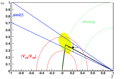
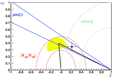
The theoretical branching ratios and the contributions of the individual channels to $\chi^{2}$ based upon these best fit values are given in table 6. The best fit parameter values are shown in table 8 together with our estimates of the errors. These errors are of course highly correlated. Plots of the error matrix ellipse for the Wolfenstein parameters $\bar{\rho}$ and $\bar{\eta}$ are shown in figures 1 and 2. The CKM angles are $\alpha=(78\pm 9)^{\circ},\;\beta=(22\pm 2)^{\circ},\;\gamma=(80\pm 7)^{\circ}$ for the BBNS model and $\alpha=(63\pm 7)^{\circ},\;\beta=(21\pm 2)^{\circ},\;\gamma=(96\pm 6)^{\circ}$ for the CP model. These can be compared with the world averages of CKMfitter $\alpha=(96\pm 13)^{\circ},\;\beta=(23.3\pm 1.5)^{\circ},\;\gamma=(61\pm 12)^{\circ}$. All errors are one standard deviation. For both models the results in table 8 for the values of the various form factors lie within the spread of theoretical estimates. The $\chi^{2}$/dof is 34.5/17 for the BBNS fit and 14.5/13 for the charming penguins.

Table 8: Best fit values and one standard deviation errors for the Beneke et al. (BBNS) and charming penguin (CP) models. $F_{\pi,K}$ and $A_{\rho,\omega,K^{*}}$ are the transition form factors $F^{B\rightarrow h}(0)$ for $P$ and $V$ mesons respectively, and $r^{\pi,K}_{\chi}$ are the chiral enhancement factors which are nominally power suppressed but are $O(1)$ in practice.

Model	$F_{\pi}$	$F_{K}$	$A_{\rho}$	$A_{\omega}$	$A_{K^{*}}$
BBNS	$0.244\pm 0.038$	$0.369\pm 0.031$	$0.344\pm 0.098$	$0.300\pm 0.094$	$0.321\pm 0.136$
CP	$0.291\pm 0.022$	$0.349\pm 0.077$	$0.320\pm 0.065$	$0.298\pm 0.072$	$0.309\pm 0.117$
	$r^{\pi}_{\chi}$	$r^{K}_{\chi}$	$A$	$\bar{\rho}$	$\bar{\eta}$
BBNS	$1.09\pm 0.24$	$1.24\pm 0.17$	$0.813\pm 0.045$	$0.068\pm 0.071$	$0.383\pm 0.090$
CP	$1.0$	$1.0$	$0.82$	$-0.044\pm 0.112$	$0.397\pm 0.050$
	$|D|$	Arg($D$)	$D^{GIM}$	Arg($D^{GIM}$)
CP	$0.068\pm 0.007$	$1.32\pm 0.10$	$0.32\pm 0.14$	$1.00\pm 0.27$

VI Discussion and Conclusions

The first conclusion is that the factorization approach works quite well. Most of the branching ratios in table 6 are predicted correctly by both models. The fitted parameters in table 8 look reasonable for both fits. The $\chi^{2}$ for the charming penguin fit is significantly better, due mainly to the poor fit of the BBNS model for the decay modes involving the $K^{*}$ meson. Also, the experimental value for $\omega K^{0}$ is not easily accomodated within the BBNS model. Both models have a problem in fitting the $\pi^{0}K^{0}$ mode. Figures 1 and 2 show the position of the apex of the unitarity triangle for both fits. The results are consistent with each other for the angle $\gamma$ but give a larger value than that suggested by the CKM Fitting Group. The angle $\beta$ agrees well for both fits.

Our theoretical best-fit values for those $CP$ asymmetries that have been measured are shown in table 9. The direct $CP$-violating parameter $A_{\text{CP}}$ for the decay channel $M_{1}M_{2}$ is

$$A_{\text{CP}}=\frac{\Gamma(\bar{B}\rightarrow\bar{M}_{1}\bar{M}_{2})-\Gamma(B\rightarrow M_{1}M_{2})}{\Gamma(\bar{B}\rightarrow\bar{M}_{1}\bar{M}_{2})+\Gamma(B\rightarrow M_{1}M_{2})}$$ (26)

where $\bar{B}=b\bar{u}$ or $b\bar{d}$. The definitions of the other $CP$-violating parameters can be found in babarcp . Regarding these asymmetries it is too early to reach a conclusion. In many cases the different experiments disagree, in others the errors are so large that a meaningful discrimination is not possible. The theoretical asymmetries are very sensitive to the parameters and to the different models and, with improved statistics, could become the final test of factorization. In table 10 we show our predictions for branching ratios and $CP$ asymmetry $A_{\text{CP}}$ for some channels not included in the fit . We include some $VV$ channels that are currently under investigation. For these channels we have assumed that the decays are to longitudinally polarized vector mesons as it is expected Cott ; Yang that decays to the other polarization states will be suppressed by at least a factor of $(m_{V}/m_{B})^{2}$.

In their most recent work Beneke and Neubert BenekePV give formulae for the weak annihilation functions $A^{i,f}_{1,3}(P,V)$ that, in addition to the terms given in (III), include terms containing a parameter $r^{V}_{\chi}$. This parameter $r^{V}_{\chi}$ has a similar origin to $r^{P}_{\chi}$ and, like $r^{P}_{\chi}$, is suppressed by a power of $\Lambda_{\text{QCD}}/m_{b}$ but, unlike $r^{P}_{\chi}$, is not chirally enhanced. We only became aware of BenekePV after completion of this study. To check for the effects of these terms we have modified our program to include the $r^{V}_{\chi}$ contribution to annihilation and have reminimized $\chi^{2}$. For the charming penguin model we found the best fit occurred with $X_{A}=1.09\exp(2.79i)$ and that there were very small changes in the best fit parameters of table 8 and the results of tables 6, 9 and 10. For the BBNS model we found similar results but the overall fit was better in that the $\chi^{2}$ was reduced from 34.5 to 27.5.

Finally, the results presented here are slightly different from preliminary numbers presented earlier moriond03 , for three reasons. The Heavy Flavour Averaging Group has updated some of the results and included a new branching fraction ($\rho^{\pm}K^{\mp}$). We have also corrected the vector-vector channels $K^{*}\phi$ for the effect of polarization. Finally we now include the systematic uncertainties in the fit.

Table 9: Measurements and theoretical best fit values for $CP$ asymmetries. Only statistical errors are shown.

$A_{\text{CP}}$	BaBar	Belle	BBNS	CP
$K^{+}\pi^{-}$	$-0.102\pm 0.05$	$-0.07\pm 0.06$	0.00	-0.08
$K^{+}\pi^{0}$	$-0.09\pm 0.09$	$0.23\pm 0.11$	0.06	-0.02
$K^{0}\pi^{+}$	$-0.17\pm 0.10$	$0.07\pm 0.09$	0.01	0.11
$\pi^{+}\pi^{0}$	$-0.03\pm 0.18$	$-0.14\pm 0.24$	0.00	0.00
$\rho^{+}\pi^{-}$	$-0.22\pm 0.08$		$-0.03$	$-0.03$
$\rho^{+}K^{-}$	$0.28\pm 0.17$		$0.10$	$-0.40$
$C_{\pi\pi}$	$-0.30\pm 0.25$	$-0.77\pm 0.27$	0.01	$-0.23$
$S_{\pi\pi}$	$0.02\pm 0.34$	$-1.23\pm 0.41$	-0.20	0.25
$C_{\rho\pi}$	$0.36\pm 0.15$		0.03	$-0.31$
$S_{\rho\pi}$	$0.19\pm 0.24$		0.38	0.65
$\Delta C_{\rho\pi}$	$0.28\pm 0.19$		0.08	0.31
$\Delta S_{\rho\pi}$	$0.15\pm 0.25$		0.02	0.11
$C_{\phi K^{0}_{s}}$	$-0.80\pm 0.38$	$0.56\pm 0.41$	$-0.01$	$-0.19$
$S_{\phi K^{0}_{s}}$	$-0.18\pm 0.51$	$-0.73\pm 0.64$	0.73	0.62

Table 10: Predicted branching ratios (in units of $10^{-6}$) and $CP$ asymmetries for some channels not included in the fit. For the $VV$ channels the predictions are for longitudinal polarization states only as these decays are expected to be dominant. The predictions are for the central values of the model fits with $1\sigma$ errors estimated by sampling the parameter error matrix.

	Mean Branching Ratio		$A_{\text{CP}}$
Decay	BBNS	CP	BBNS	CP
$\pi^{0}\pi^{0}$	$0.5\pm 0.1$	$1.1\pm 0.2$	$0.59\pm 0.08$	$-0.63\pm 0.15$
$\rho^{0}\rho^{0}$	$0.5\pm 0.1$	$1.2\pm 0.3$	$0.69\pm 0.16$	$-0.66\pm 0.07$
$\pi^{0}\rho^{-}$	$8.4\pm 0.7$	$11.9\pm 1.4$	$0.04\pm 0.01$	$0.06\pm 0.01$
$\rho^{0}\rho^{-}$	$19.0\pm 3.1$	$17.8\pm 3.3$	$0.00\pm 0.00$	$0.00\pm 0.00$
$\rho^{0}K^{+}$	$2.0\pm 0.6$	$4.6\pm 0.5$	$0.00\pm 0.09$	$-0.01\pm 0.64$
$\rho^{0}K^{*+}$	$4.6\pm 1.3$	$5.2\pm 0.7$	$0.33\pm 0.06$	$-0.35\pm 0.06$

Figure 1: Result for the unitarity triangle fit in the BBNS model. The shaded area shows the $3\sigma$ allowed region for the apex of the unitarity triangle. The data point shows the fit result from the unitarity triangle fit from other measurements taken from CKMfitterCKMfitter .

Figure 2: Result for the unitarity triangle fit in the charming penguin model. The shaded area shows the $3\sigma$ allowed region for the apex of the unitarity triangle. The data point shows the fit result from the unitarity triangle fit from other measurements taken from CKMfitterCKMfitter .

References

• (1) W. N. Cottingham, I. B. Whittingham, N. de Groot and F. Wilson, J. Phys. G:Nucl. Part. Phys. 28, 2843 (2002).
• (2) M. Beneke, G. Buchalla, M. Neubert and C. T. Sachrajda, Nuc. Phys. B 606, 245 (2001).
• (3) D. Du, H. Gong, Y. Sun, D. Yang and G. Zhu, Phys. Rev. D 65, 074001 (2002).
• (4) D. Du, H. Gong, Y. Sun, D. Yang and G. Zhu, Phys. Rev. D 65, 094025 (2002); Phys. Rev. D 66, 079904(E) (2002).
• (5) D. Du, H. Gong, Y. Sun, D. Yang and G. Zhu, Phys. Rev. D 67, 014023 (2003).
• (6) R. Aleksan, P.-F. Giraud, V. MorΓ©nas, O. PΓ¨ne and A. S. Safir, Phys. Rev. D 67, 094019 (2003).
• (7) X.-H. Guo, O. M. A. Leitner and A. W. Thomas, hep-ph/0307201
• (8) M. Beneke and M. Neubert, hep-ph/0308039.
• (9) P. Ball, J. High Energy Phys., 69, 005 (1998).
• (10) C-D. LΓΌ and M-Z Yang, hep-ph/0212373.
• (11) A. Ali and C. Greub, Phys. Rev. D 57, 2996 (1998); A. Ali, G. Kramer and C-D. LΓΌ, Phys. Rev. D 58, 094009 (1998).
• (12) M. Ciuchini, E. Franco, G. Martinelli, M. Pierini and L. Silvestrini, Phys. Lett. B 515, 33 (2001); hep-ph/0110022; hep-ph/0208048.
• (13) A. J. Buras and L. Silvestrini, Nuc. Phys. B 569, 3 (2000).
• (14) The BaBar Collaboration (B. Aubert et al.), hep-ex/0307026.
• (15) Heavy Flavour Averaging Group, http://www.slac.stanford.edu/xorg/hfag/index.html.
• (16) F. James and M. Roos, MINUIT, CERN D506, CERN Program Library Office, CERN, CH-1211 Geneva 23, Switzerland.
• (17) http://ckmfitter.in2p3.fr/
• (18) N. de Groot, W. N. Cottingham and I. B. Whittingham, hep-ph/0305263.
• (19) The BaBar Collaboration (B. Aubert et al., hep-ex/0207068.
• (20) K. C. Yang, hep-ph/0308095