TASI Lectures on Effective Field Theories

Abstract

These notes are a written version of a set of lectures given at TASI-02 on the topic of effective field theories. They are meant as an introduction to some of the latest techniques and applications in the field.

Prelude

It is a little known fact that the Pioneer spacecraft launched in the mid-seventies contains a data repository with a summary of human scientific knowledge. It is interesting to ask what would happen if an alien civilization found this satellite and studied its contents? Let us furthermore suppose that while these aliens were/are greatly advanced technologically, they are not terribly well versed in basic research, mainly because of the alien government’s short-sightedness and are thus very interested in the free knowledge that we are offering them. One of the pieces of information in the data repository is a copy of the particle data group booklet (the hand sized one, not the tome). The booklet is handed over to the relevant scientists, and a massive project is launched to decipher the information. After a couple of years of going over the data and a copy of Bjorken and Drell, which was also on board, the aliens are up to speed and ready to test our theories. They’ve come to the conclusion that we claim to have a well defined theory of strong and electro-weak interactions up to the TeV scale (let’s not quibble over anachronisms), and that while we don’t know exactly what happens at the TeV scale there is something that unitarizes the theory above that scale. They also conclude that our understanding of gravity is very limited. In particular, while we know how to calculate quantum corrections at energies which are small compared to the Planck scale, above the Planck scale we have no idea what is going on.

After some period of intense investigations, the aliens decide to test the theoretical predictions based on what they learned from us. A proposal is put forward by a prominent experimentalist for a high precision measurement of the level splittings in Hydrogen. The proposal is summarily rejected based on a review written by a top alien theorist. The rejection was based on the referee’s argument that it is silly to try to calculate loop corrections in the human’s field theory. The referee’s justification for this statement is that given that gravitons run through the loops and the fact the integrals include momenta above the Planck scale, where we know the theory breaks down, there is no way that one can expect that the results will be correct. Moreover, even if gravitational couplings are suppressed by the Planck scale, there are power law divergences which can compensate for these suppressions, so it seems that any attempt at calculating loop corrections would be fruitless. Fortunately, for us, there were some wise aliens working at the funding agency, and they said, “let’s for the moment ignore gravitational effects, and see if the data agrees with what we get using just electro-magnetic effects”. So the experiment was done and the theory did indeed meet with great success.

So where did the referee go wrong? Well, to be fair, the referee was not completely wrong. There is a kernel of truth to its claims. It is true that the theory breaks down and that we should indeed pause to think about the results of any calculation which involves loop momenta above the Planck scale (the scale where the theory is no longer reliable). Since we know we are not correctly portraying the physics at the high scale, whatever the result of the loop integration may be, it will have to be treated in some way so as to remove the dependence on the UV physics. Indeed, the loop integrals will, in general, be divergent and need to be regulated. But there is no preferred regulation procedure and, therefore, the numerical value of the integral is ambiguous. However, the point the referee missed is that if we are not too ambitious, this is not a problem. The short distance physics, which is not properly accounted for in the loop integrals, looks local at low energies. Another way of saying this is, that if we think of the loop integral in coordinate space, the part of the integral from which we know we are getting nonsense can be contracted to a point and therefore looks like an insertion of a local operator into our Feynman diagram. This means that all of the effects of the unknown short distance physics can be mimicked by adding some new operators into our Lagrangian (as we will see these operators may be of arbitrarily high dimensions). That is to say, all the effects of the short distance physics can be accounted for by either shifting the parameters in our renormalizable Lagrangian, or by adding higher dimensional operators which are suppressed by the UV scale, $M_{UV}$. Since we needed to perform measurements to fix those parameters anyway we still have predictivity as long as we truncate the Lagrangian at some order in powers of $1/M_{UV}$. So we see now in what way the referee was right. It’s not that the unknown effects of the short distance physics are parametrically small in any way, indeed these effects are very important as they contribute at order one to the parameters in the renormalizable part of the Lagrangian. It’s that all the effects go into making up the electron mass and all the other low energy parameters of the theory . If you changed the short distance physics it could, and would, change the values of the low energy parameters. Thus, as long as we are not too ambitious, we don’t need to worry about the fact that our integrals diverge! Who cares if they diverge, we didn’t expect to get the answer right anyway. So we should really call our field theories “effective” field theories. This moniker warns the consumer that it should be used with caution, as at some scale the theory no longer makes any sense. What that scale is depends upon the interactions one is trying to describe.

Let’s for the moment consider a universe where the effects of short distance physics could not be absorbed into low energy parameters. We couldn’t calculate anything without knowing the complete theory of quantum gravity. While, this line of reasoning seems almost obvious now, thinking in terms of effective field theories (EFT) only became generally accepted in the last few decades. Indeed, from an EFT point of view, renormalizability, which was a standard benchmark for acceptable quantum field theories not that long ago, is no longer relevant, unless we’re interested in theories which are supposed to correctly describe all the short distance physics. Does this mean that field theory as a mathematical construct is incapable of being a “complete” theory? Certainly not. There are many field theories which are valid to arbitrarily high scales. The classic examples being asymptotically free theories such as QCD. These theories possess trivial UV fixed points, which allow for the cut-off to be taken to infinity. In fact, the necessary criteria for completeness is the existence of a UV fixed point, and taking the cut-off to infinity is called taking the “continuum limit”, following the lattice terminology. The reasoning behind this criteria is that at the fixed point, the correlation length $\xi$, (read inverse mass) diverges, and thus one can study physics at arbitrarily large distances compared to the cut-off (the inverse of the lattice spacing $a$), which is equivalent to saying that the cut-off can be taken to infinity since lattice artifacts will be suppressed by powers of $\xi/a$Wilson . Of course if we want a “theory of everything”, it can’t be asymptotically free since we know that gravity should become stronger in the UV. Thus, any quantum field theory description of gravity should possess a non-trivial UV fixed point. This possibility is very difficult, or perhaps impossible to rule out. Presently, the consensus is that it may well be that a local quantum field theory is not capable of describing physics at and above the Planck scale. However, field theory is profoundly rich, and I would guess it still possesses many tricks which have yet to be revealed to us.

I Lecture I: The Big Picture

This lecture is meant to give a global overview of effective field theories. The first part of the lecture in an introduction to the basic idea and a tutorial on the matching procedure, all discussed within the context of a simple toy scalar model. I then categorize the various types of effective field theories into two main headings depending upon whether the theory admits a perturbative matching procedure. Most of the rest of the lecture is dedicated to some sample theories where we can match. I will assume throughout these lectures that the reader has a basic understanding of renormalization.

I.1 A Toy Model

Let us now try to be more quantitative by starting with a simple toy model. What we would like to illustrate is that all the effects of ultra-violet (UV) physics may be absorbed into local counter-terms and furthermore, that all of the physical effects of the UV physics are suppressed by powers of the UV scale. To do so we will work with a model of two scalar fields , $\Phi_{L}$ and $\Phi_{H}$, with $m_{H}\gg m_{L}$, in four dimensions. The interaction Lagrangian will be given by

$$-{\it L}_{int}=\frac{\lambda_{0}}{4!}\Phi_{L}^{4}+\frac{\lambda_{1}}{2}\Phi_{H}\Phi_{L}^{2}+\frac{\lambda_{2}}{4}\Phi_{L}^{2}\Phi_{H}^{2}+\frac{\lambda_{3}}{4!}\Phi_{H}^{4}.$$ (1)

It is typical, in most pedagogical treatises, to impose a discrete symmetry to forbid tri-linear interactions, as such terms introduce dimensionful couplings, which complicate the systematics. However, such interactions will illuminate certain ideas which otherwise would not arise until higher orders in the loop expansion. The usual problems with tri-linear theories arise from issues of vacuum stability, but for our purposes these issues will not be an obstruction.

I will assume that all the couplings, except for $m_{L}$, take on their “natural values”. Here I use the term “natural” in both the sense of Dirac and t’Hooft. That is, dimensionless couplings should be of order one (Dirac) and dimensionful couplings should be of order of the largest scale in the problem, unless a symmetry arises in the limit when the coupling vanishes (t’Hooft). Thus, we take $\lambda_{2}\simeq 1$ and $\lambda_{1}\simeq m_{H}$. Furthermore, since there is no symmetry protecting the light scalar mass, choosing $m_{L}\ll m_{H}$ is unnatural, but this is just an aesthetic issue with which we wont be bothered.

Now, according to the arguments in the previous section, it should be possible to write down a local theory involving only the light degrees of freedom which correctly reproduces the physics of the full theory as long as we only consider external momenta much less than $m_{H}$. The process of determining the low energy theory is called “matching”, and the strategy is quite simple. We build up our low energy theory, which only involves the light fields, such that it reproduces the full theory up to some orders in $(p,m_{L})/m_{H}$ and $\lambda_{i}$ where $p$ is the external momentum of the process under consideration which we will take to be of order $m_{L}$. Doing this is quite simple in practice. The effective theory action will be given by the full theory action with all heavy fields set to zero plus some new terms which account for the effects of the heavy fields. The additional terms are determined order by order in perturbation theory by calculating some amputated Greens function in the full and effective theories and taking the difference

$$\delta L_{EFT}={\rm Full~{}Theory~{}Result}-{\rm Effective~{}Theory~{}Result.}$$ (2)

In a sense what the left hand side of this equation is telling you is exactly what the effective theory is missing. Since the effective theory is designed to reproduce the IR physics of the full theory, $\delta L_{EFT}$ will have a well defined Taylor expansion around $p=0$. Thus the holes in the effective theory can be plugged by adding local operators. If this seems a little obscure at this point don’t worry as we will discuss many concrete examples of this matching procedure below.

Notice that matching each n-point function will generate distinct local operators in the effective theory, with higher n-point functions obviously generating higher dimensional operators. Thus the number of n-point function one needs to calculate depends upon the desired accuracy. The more accuracy we want the more operators we must keep, as each operator of successively higher dimension will be suppressed by additional powers of the UV scale.

Let’s see how this works in our toy theory. Consider the amputated four point function for the light fields. At tree level, there are four diagrams which contribute to this process. One is the usual contribution involving only the light fields gives $-i\lambda_{0}$, and the other three have intermediate heavy scalars as shown in figure (1). These latter contributions are given by

$$\textrm{Fig 1}=\frac{-i\lambda_{1}^{2}}{s-m_{H}^{2}}+s\rightarrow(t,u).$$ (3)

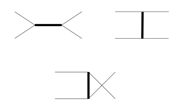
Figure 1: Tree level contributions to the full theory four point functions involving the heavy scalar (thick lines).

After expanding (3) we can see that the four point function can be reproduced, up to corrections of order $p^{2}/m_{H}^{2}$ by using

$$\delta L_{int}=C_{4}^{(1,0)}\frac{\Phi_{L}^{4}}{4!}~{}~{}~{}~{}~{}$$ (4)

Here I have established notation for the coefficients (called “Wilson coefficients”), the subscript counts the number of fields while the superscripts denote the order in the expansion in coupling and derivatives (more generally powers of $1/m_{H})$, respectively. We can now see clearly what was emphasized in the introduction. As far as a low energy observer is concerned this looks like a simple $\Phi^{4}$ theory with a coupling that we had to fix via experiment anyway. The low energy observer would be completely oblivious to the UV physics unless the experiment were sensitive enough to see the deviations from $\Phi^{4}$ theory due to $p/m_{H}$ corrections. If we wanted to, we could add additional operators to ensure that we correctly reproduce the higher n point functions as well. Suppose the low energy observer upgrades the machine, either by raising the energy or luminosity, to the point where the data can no longer be fit by pure $\phi^{4}$ theory. We know exactly what to do to correctly reproduce the data, simply add the higher derivative interaction

$$\delta L_{int}=\frac{C_{4}^{(1,2)}}{m_{H}^{2}}\frac{\Phi_{L}^{2}\partial^{2}\Phi_{L}^{2}}{4!}.$$ (5)

Other operators with two derivatives and four fields can all be put into the form above via integration by parts and use of the equation of motion. That this latter manipulation is allowed will be discussed later.

As the energy of the experiment is further raised one needs to include higher and higher derivative interactions to reproduce the data. Notice that until we get to high enough energies to actually produce the heavy scalar we will be in the dark as to the true underlying theory. This is because in principle there will be an equivalence class ( called a ”“universality class”) of theories which look the same in the infra-red. As we fit more and more of the couplings of the higher dimension operators we would be able to eliminate theories, but removing all ambiguities would be difficult without including some other selection criteria.

So far, we’ve shown that to tree level we can reproduce the full theory by adjusting coefficients in an effective Lagrangian, this is called “matching”. This matching procedure can be carried out to arbitrary order in the couplings and $p/m_{H}$. Indeed, suppose we wish to match at higher orders in the couplings. The matching procedure now takes on a new twist, but the idea is the same. We Taylor expand the full theory result and compare it to the result in the effective theory. We then modify the effective theory so as to get the answer right. I should mention at this point that in most theories the loop and coupling expansions coincide. But in our toy model, because of the $\lambda_{1}$ coupling this is no longer true. Nonetheless we can overcome this issue by assuming that ($\lambda_{1}/m_{H}\equiv\hat{\lambda}_{1}$) is of order $\sqrt{\lambda_{0}}$. In this way all tree level contributions are of order $\lambda_{0}\simeq\lambda_{2}\simeq\lambda_{3}$. This is why I labelled the Wilson coefficient above $C_{4}^{(1,2)}$.

Returning to our calculation, let us see if we can reproduce the full theory at next order in the couplings, beginning with the two point function. There are two leading order (dimension four) operators which get renormalized when calculating the two point function. The mass $m_{L}^{2}\Phi_{L}^{2}$ and the kinetic energy $\Phi_{L}\partial^{2}\Phi_{L}$. The one loop contributions to the two point function are shown in figure (2).

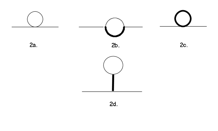
Figure 2: One loop contributions to the full theory two point function.

Diagram 2a. is the usual contribution found in $\Phi^{4}$ theory and is given by

$$\textrm{Fig 2a.}=\frac{i\lambda_{0}m_{L}^{2}}{32\pi^{2}}\left(\frac{1}{\overline{\epsilon}}-\ln(\frac{m_{L}^{2}}{\mu^{2}})+1\right)$$ (6)

where I will use the notation

$$\frac{1}{\overline{\epsilon}}=\frac{1}{\epsilon}-\gamma+\ln(4\pi).$$ (7)

The diagram in 2c. gives the same result as 2a., but with the replacement $(m_{L},\lambda_{0})\rightarrow(m_{H},\lambda_{2})$. Both of these contributions are momentum independent and thus only renormalize the mass. Figure 2b, on the other hand, will have non-trivial momentum dependence. We expect to have a cut beginning at $(m_{H}+m_{L})^{2}$, and thus this contribution will be analytic in the neighborhood $p^{2}\simeq m_{L}^{2}$. Doing the one-loop integration gives

$$\textrm{Fig 2b.}=\frac{i\lambda_{1}^{2}}{16\pi^{2}}\left(\frac{1}{\overline{\epsilon}}-\ln(\frac{m_{H}^{2}}{\mu^{2}})+1\right)$$ (8)

where I have expanded in $1/m_{H}$, and kept only the leading term. Finally, there is a contribution from the tadpole diagram 2d. which is given by

$$\textrm{Fig 2d.}=-\frac{i\lambda_{1}^{2}}{32\pi^{2}}\frac{m_{L}^{2}}{m_{H}^{2}}\left(\frac{1}{\overline{\epsilon}}-\ln(\frac{m_{L}^{2}}{\mu^{2}})+1\right).$$ (9)

Now let’s calculate in the effective theory. We must note that to be consistent we must use the $O(\lambda)$ effective Lagrangian which we generated at tree level when we calculate on the effective theory side (the aforementioned twist). This is in contrast to the tree level matching where there is nothing to calculate on the effective theory side. At leading order in $1/m_{H}$, the only relevant operator is the $\Phi_{L}^{4}$ term and so we find that the effective theory gives the same result as Fig 2a. except now the coupling is not $\lambda_{0}$ but $C_{4}^{(1,0)}$. To match we take the renormalized (here in $\overline{MS}$) full theory result expanded around small ($\hat{m}_{L}^{2},\hat{p}^{2}=p^{2}/m_{H}^{2}$), and subtract the renormalized effective theory result, finding

$$C_{m}^{(1,0)}\!=\!\frac{1}{32\pi^{2}}\left[\!\lambda_{2}m_{H}^{2}\left(1-\ln(\frac{m_{H}^{2}}{\mu^{2}})\right)-\lambda_{1}^{2}\left(2\ln(\frac{m_{H}^{2}}{\mu^{2}})\!-\!2\!-2\frac{m_{L}^{2}}{m_{H}^{2}}(\ln\frac{{m_{L}^{2}}}{\mu^{2}}+1)\right)\!\right].$$

To insure that perturbation theory is well behaved, we should choose $\mu$ to minimize the large logs. This scale is called the “matching scale”. Intuitively we would think that this scale should be the high scale $m_{H}$. Given that the effective theory is supposed to reproduce the infrared physics, we would expect that all the dependence on the low energy parameter $m_{L}$ should be identical on both sides of the matching equation, thus leaving all logs in the matching independent of $m_{L}$. However a glance at our results shows that choosing $\mu=m_{H}$ does not get rid of all the large logs. Clearly we have done something wrong. The problem stems from the fact that we have kept some terms which we had no business keeping. In particular, diagram 2d. is power suppressed relative (remember that $\lambda_{1}$ scales as $m_{H}$) to the other diagrams. Thus, to be consistent we need to expand our full theory result for diagram 2b. to one more order. So we make the replacement

$$\textrm{Fig 2b.}\rightarrow\textrm{(8)}+i\frac{\lambda_{1}^{2}}{16\pi^{2}}(\frac{m_{L}^{2}}{m_{H}^{2}}\ln\frac{m_{L}^{2}}{m_{H}^{2}}).$$ (11)

The log term will exactly kill off all of the large logs in $C_{m}^{(1,0)}$, leaving

$$C_{m}^{(1,0)}=\frac{1}{16\pi^{2}}\lambda_{1}^{2}(1+\frac{m_{L}^{2}}{m_{H}^{2}})+\lambda_{2}\frac{m_{H}^{2}}{32\pi^{2}}.$$ (12)

Notice that this correction wants to pull up the light scalar mass to the scale $m_{H}$ since $\lambda_{1}\simeq m_{H}$. This is just what we called “unnatural” in the sense of t’Hooft, since as $m_{L}$ is taken to zero we do not enhance the symmetry. Keeping $m_{L}\ll m_{H}$ will require a fine tuning of the counter-terms at each order in perturbation. In the $\overline{MS}$ scheme this wont show up until we try to relate the $\overline{MS}$ mass to the physical mass. That is, there will be a relation of the form

$$m_{L}^{2~{}(phys)}=m_{L}^{2~{}\overline{MS}}+O(\lambda/(32\pi^{2}))(m_{H}^{2}),$$ (13)

and we will need to delicately choose $m_{L}^{2~{}\overline{MS}}$ to cancel the large $O(m_{H}^{2})$ piece.

The momentum dependent terms will simply shift the field normalization in the effective theory with $C_{p}^{(1,0)}=\frac{\lambda_{1}^{2}}{32\pi^{2}m_{H}^{2}}$. If we wish to go to higher orders in the $1/m_{H}$ expansion we will generate the operator

$$O_{2}=C_{2}^{(1,2)}\Phi_{L}\frac{\nabla^{4}}{m_{H}^{2}}\Phi_{L}.$$ (14)

Exercise 1.1: Calculate $C_{2}^{(1,2)}$

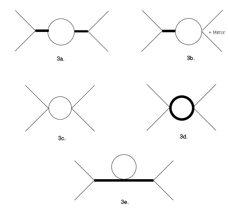
Figure 3: A partial list of the one loop contributions to the full theory four point functions.

Now let us consider the four point function. A partial list of the relevant full theory diagrams are shown in figure 3.The diagrams with external leg corrections will automatically be reproduced by the effective theory, since we already matched the two point function. In the effective theory, there will be only one diagram, and it is identical to 3c. except that at each vertex we use the coupling $C_{4}^{(1,0)}$. By considering the combination of couplings coming from $(C_{4}^{(1,0)})^{2}$, we can begin to see that we will indeed reproduce 3a, 3b and 3c. However, we can also see that this diagram will not be able to reproduce the log of $m_{L}$ from figure 3e. To match this log we will have to first reproduce the six point function at tree level. Then diagram 3e. will be reproduced by tying together two external legs. You can see how this will happen by noting that heavy field propagators can be contracted to a point in the full theory graph. Figure 3d will have no partner in the effective theory and will contribute ( in the s channel), after renormalization and expansion in $\hat{s}\equiv\frac{s}{m_{H}^{2}}$,

$$\textrm{Fig 3d.}=-\frac{i\lambda_{2}^{2}}{16\pi^{2}}\left(\ln(\frac{m_{H}^{2}}{\mu^{2}})-\frac{\hat{s}}{6}+\cdot\cdot\cdot\right).$$ (15)

We see that since we are matching at the scale $\mu=m_{H}$, this diagram will not contribute to $C_{4}^{(2,0)}$, at least in the $\overline{MS}$ scheme. The other channels give similar contributions.

Exercise 1.2 First draw all the remaining diagrams which contribute to the four point function in the full theory. Then show that all the dependence on $\ln(m_{L})$ cancels in the matching for the four point function. Hint: By working at zero external momentum the calculation greatly simplifies.

What happens if we go to first order in $p^{2}/m_{H}^{2}$, staying at one loop? At this order when we calculate in the effective theory, we will need to include the graph depicted in figure 4, where the circle represents an insertion of the operator (5). The integral for this Feynman diagram will have a contribution which is quadratically divergent

$$I_{\Lambda^{2}}=\int\frac{d^{4}p}{(2\pi)^{4}}\frac{p^{2}}{(p^{2}-m_{H}^{2}+i\epsilon)((p_{1}+p_{2}+p)^{2}-m_{H}^{2}+i\epsilon)}.$$ (16)

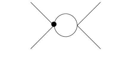
Figure 4: One loop contributions to the effective theory four point functions, with the dark circle representing an insertion of the derivative operator (5).

Now, suppose we regulate this divergence with a cut-off, then this contribution will scale as $\Lambda^{2}/m_{H}^{2}$. What order is this in our momentum expansion? If it’s order one, it would seem that we have lost all hope of calculating in a systematic fashion, since no matter how many powers of $m_{H}$ may suppress a given operator, it may give an order one contribution if we stick it into a multi-loop diagram. This would be a disaster. However, this reasoning is misleading. The fact that something can’t be right can be immediately seen by working with a different regulator. Suppose we work in dimensional regularization. In this scheme, there are no power divergence as they are automatically set to zero Sterman . It had better not be that our answer depends on our choice of regulator, otherwise we’re clearly lost. So what’s going on? Which regulator is giving us the correct result? The answer is, both. The difference between the two is “pure counter-term”, which means the discrepancy in the two results can be accounted for by a shift in the couplings of local operators. Since the couplings are measured, and not predicted, there is no physical distinction between the two results. The only difference is in the bookkeeping, that is, the counter-terms in the two schemes differ but that’s it. The nice thing about dimensional regularization is that we don’t have to worry about mixing orders in $1/m_{H}$. We can see that if we use a cut-off and take it to be of order $m_{H}$, then operators which are formally suppressed will “mix up” with operators of lower dimension. But if we stick to dimensional regularization, then powers of $1/m_{H}$ are explicit, as they only appear in coefficients of operators (modulo the caveat about $\lambda_{1}$ in our toy theory), so we can read off the order of a loop diagram immediately. Thus, in general it is wiser to always work in “dim. reg.” when doing effective field theory calculations. This is not to say that the cut-off doesn’t have its time and place. In particular the cut-off makes quadratic divergences explicit, whereas in dim. reg. they show up as poles in lower dimensions.

Another interesting point which arises from the calculation of the diagrams in figure 4 is the fact that there are divergences which can only be subtracted using counter-terms for operators with dimensions greater than four. The effective theory is non-renormalizable, an anathema in ancient times. That is, there are new UV divergences in the effective theory that arise in each order of perturbation theory. These divergences were not there in the full theory. This should not surprise us, since the effective theory is only built to mock up the IR of the full theory, not the UV. Thus the UV divergences will not cancel in the matching. This isn’t a problem, we simply choose a scheme, and subtract. In the effective field theory approach we should be careful with out choice of scheme. If we’re not careful we could mess up our power counting by introducing a scale. So we should choose a nice simple mass independent scheme like $\overline{MS}$. I will have more to say about this later on in these lectures. Notice that the matching coefficient will clearly be prescription dependent, but any such prescription dependence will drop out in low energy predictions.

Exercise 1.3 Calculate the anomalous dimensions of the dimension six operator $\Phi_{L}^{2}\partial^{2}\Phi_{L}^{2}$ to one loop. The additional UV divergences which arise in the effective theory correspond to IR divergences in the full theory. This is easily understood from the fact that we have taken $m_{H}$ to infinity in the effective theory. So the “IR” divergence $\ln(m_{H})$ now looks UV. Thus effective field theory allows us to resum IR logs in a simple way using standard renormalization group techniques. We will see an example of this in the coming sections.

I.2 Matching on or off the mass shell?

Before moving on I’d like to discuss one more technical aspect of matching. In particular, it’s important to understand that it doesn’t matter whether or not one chooses to match with external states on-shell or off-shell. The reason is that putting external lines off-shell only changes the IR behavior of the theory, and since the effective theory is designed to reproduce the non-analytic structure of the full theory, all the information regarding the virtuality of the external lines cancels in the matching. This can greatly reduce the amount of work one has to do to match. For instance, if one is not interested in matching operators with derivatives, then one could choose the external momenta to vanish identically, greatly simplifying the necessary integrals. Also if one matches off-shell one can induce operators in the effective theory which vanish by the leading order equations of motion. For example, in our toy model we could induce $\Phi_{L}^{3}\partial^{2}\Phi_{L}$. However, it is quite simple to show that we can eliminate this operator via a field redefinition, which are known to leave S-matrix elements unchanged due to the equivalence theoremequiv . The proof GeorgiI is inductive. Suppose we have set all operators of order $(p/m_{H})^{n}$ which vanish by the leading order equations of motion (by leading order I’m referring to the momentum expansion) to zero. If there exists an operator at order $(p^{2}/m_{H}^{2})^{n+1}$ of the form $F(\Phi_{L},\Phi_{H})\partial^{2}\Phi_{L}$, then we make the field redefinition

$$\delta\Phi_{L}=-F(\Phi_{L},\Phi_{H})$$ (17)

so that variation of the leading order Lagrangian

$$\delta L^{LO}=(\delta\Phi_{L})\partial^{2}\Phi_{L}$$ (18)

exactly cancels the offending term. Notice that since $F$ is order $n+1$ in the derivative expansion the lower order operators remain unchanged but we do induce a change in the subleading set of operators, i.e. at order $n+2$. However, since in an effective theory we generate all possible operators consistent with the symmetries, all this redefinition will do is to shift the value of some matching coefficients.

I.3 Non-Decoupling and Wess-Zumino Terms

Let us consider the case of a chiral gauge theory. These are theories for which a fermion mass term is disallowed by gauge invariance. We know that if the theory is to be unitary and gauge invariant, the particle content must be such that all the gauge anomalies arising from triangle diagrams sum to zero. The classic example of such a theory is the standard model itself, where the fermions get their masses from the Higgs Yukawa couplings. Taking the fermion masses large while holding the symmetry breaking scale fixed corresponds to the limit of a large Yukawa coupling $\lambda$. Since the coupling is proportional to the mass, we might expect that low energy observables (below the scale of symmetry breaking) could be enhanced by a large mass. The classic example of this “non-decoupling” arises in $K-\bar{K}$ mixing. After integrating out the top quark one generates a term in the $\Delta S=2$ Hamiltonian

$$H_{t}=m_{t}^{2}\frac{G_{F}^{2}}{16\pi^{2}}\eta_{2}O_{4},$$ (19)

where $O_{4}$ is a four quark operator. A similar effect shows up in the $\rho$ parameter, which is a measure of the ratio of charged to neutral currents. These effects would disappear in the limit where the bottom and top quark become degenerate, the former vanishes as a consequence of the GIM mechanism. Both of these effects arise due to $SU(2)$ breaking. If we took the limit where both the bottom and the top quark masses become equal and large, then we would expect that the effects of this heavy pair could all be absorbed into $SU(2)$ symmetric operators.

The thoughtful reader might be confused by this last statement if they are familiar with anomalies. Suppose that one of the $SU(2)_{L}$ doublets is much heavier than the weak scale, and we wish to integrate it out. The low energy theory would then have anomalous matter content and would apparently no longer be gauge invariant. Actually things can look even worse. If we start with an even number of $SU(2)_{L}$ doublets and integrate out one such pair, then naively, the partition function would vanish due to the non-perturbative anomaly Witten . . Now it should not come as no surprise that at “low energies” we do not have manifest gauge invariance. Nor should we be worried about this fact, since the lack of gauge invariance will only manifest itself in a pernicious way (a breakdown of unitarity) at energies near the masses of the gauge bosons. Nonetheless we should be able to add a tower of higher dimensional operators which will allow us to calculate sensibly at energies above the masses of the gauge bosons. The question is, what scale suppresses the effects of the fermions in these higher dimensional operators? The answer is the symmetry breaking scale $v$, and not the mass of the fermion. Integrating out a heavy fermion will generate a set of higher dimensional operators such as those arising from the graph in figure (5).

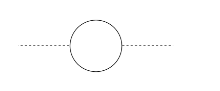
Figure 5: A diagram which contributes to a dimension six operator which is suppressed by $1/v^{2}$.

This graph will generate a whole string of operators once we expand it in momentum. Consider the contribution to the dimension 6 operators, which are suppressed by $1/M_{UV}^{2}$. Just from counting vertices and dimensional analysis we see that it must scale as $1/M_{UV}^{2}\propto\lambda^{2}/m^{2}=1/v^{2}$. Thus we can’t write down a local effective theory which is valid in the region $v<E<\lambda v$, at least with these variables. The trouble all starts from the fact that fermions are getting their relatively large masses from dimensionless couplings. Even so, we should be able to calculate in a reliable fashion up to the scale $v$ even with our low energy theory which appears anomalous.

Imagine we’re taking the limit $g\ll 1$ so that there is a large hierarchy between $M_{W}$ and $v$, and we wish to calculate in this window. How can we recover a sensible theory without the heavy fermion pair? The answer is via a “Wess-Zumino” term WZ . In the present context the generation of this term was worked out in a series of papers by D’Hoker and Farhi, which I will only briefly summarize. The serious student may wish to spend some time looking at the original work DF .

If we allow for $\lambda\gg 1$, then the heavy fermions will be strongly coupled, but this should not stop us from matching onto an effective theory. We know that we will not be able to match perturbatively. However, the large $\lambda v$ limit lends itself naturally to a derivative expansion which will keep our matching under control. We will simplify the problem by considering a toy Yukawa theory with $SU(N)_{L}\times SU(N)_{R}$ symmetry. The field content is a left (right) handed fermion in the fundamental and a Higgs in the bi-fundamental, which transform as

$$\psi_{L}\rightarrow g_{L}\psi_{L},~{}~{}~{}~{}~{}\psi_{R}\rightarrow g_{R}\psi_{R},~{}~{}~{}~{}~{}\Phi\rightarrow g_{L}\Phi g^{\dagger}_{R},$$ (20)

$g_{L}$ and $g_{R}$ are independent elements of $SU(N)_{L}$ and $SU(N)_{R}$ respectively. The addition of gauge fields complicates things only slightly. The action for the model is given by

$$\textsl{L}=i\overline{\psi}_{L}\partial\!\!\!/\psi_{L}+\overline{\psi}_{R}i\partial\!\!\!/\psi_{R}-\lambda\overline{\psi}_{L}\Phi\psi_{R}-\lambda\overline{\psi}_{R}\Phi^{\dagger}\psi_{L},$$ (21)

where the Higgs doublet, $\Phi$ is written as $\Phi=vU$, with $U$ being a unitary matrix. That is we have frozen the modulus of the Higgs field to simplify the problem. Allowing the modulus to fluctuate wont change our conclusions.

Now we would like to match on to an effective theory without the heavy fermions. The matching involves only calculations in the full theory since the are no graphs in the effective theory. If we were working in the standard model and wanted only to integrate out the top quark, this would no longer be true. Thus matching corresponds to formally do the path integral over the fermions then expanding the effective action

$$W(U)=-i\ln\int d[\psi_{L}]d[\psi_{R}]exp\left(i\int d^{4}x\textsl{L}\right)$$ (22)

in powers of $1/(\lambda v)$, keeping only the terms which do not vanish in the $\lambda\rightarrow\infty$ limit. Here I will only sketch how this calculation is done. The trick is to perform a change of variables to absorb the Higgs field into a gauge field. This is accomplished by the redefinition

$$N_{L}=U^{\dagger}\psi_{L},~{}~{}~{}N_{R}=\psi_{R},$$ (23)

which results in

$$\textsl{L}=\overline{N}_{L}(i\partial\!\!\!/-A\!\!\!/_{L})N_{L}+\overline{N}_{R}i\partial\!\!\!/N_{R}-\lambda v(\overline{N}_{L}N_{R}+\overline{N}_{R}N_{L}),$$ (24)

where $A_{L}=U^{\dagger}\partial^{\mu}U$. The advantage of using this form is that a derivative expansion corresponds to an expansion in the number of external fields.

We may write the new effective action defined in terms of an integral over the $N$ fields, as $W^{\prime}$ with

$$W=W^{\prime}-iJ(U)$$ (25)

since

$$[d\psi_{L}]=J(U)[dN_{L}].$$ (26)

Where $J(U)$ is the Jacobian for the change of variables (23). $W^{\prime}$ can be calculated using the usual Feynman diagram techniques, and, in general, contains many interesting pieces, such as the famous “Goldstone-Wilzcek” current GW which can endow solitons with fermion number. However, in this model, all of these terms will be invariant under the anomalous symmetry, so we will not concern ourselves with them at present. We will be mostly concerned with the Wess-Zumino term which resides in the JacobianWZ . This term can not be written as the four dimensional integral of an $SU(2)\times SU(2)$ invariant density but can be written as an invariant five dimensional integral Witten2

$$\Gamma_{WZ}=\frac{-i}{240\pi^{2}}\int d^{4}x\int_{0}^{1}dx^{5}\epsilon^{abcde}Tr\left[\tilde{U}^{\dagger}\partial_{a}\tilde{U}\tilde{U}^{\dagger}\partial_{b}\tilde{U}\tilde{U}^{\dagger}\partial_{c}\tilde{U}^{\dagger}\tilde{U}\partial_{d}\tilde{U}\tilde{U}^{\dagger}\partial_{e}\tilde{U}\right].$$

$\tilde{U}$ is an arbitrary (differentiable) extension of $U$ into the $x^{5}$ direction which need only to satisfy

$$\tilde{U}(x^{5}=0,x^{\mu})=1~{}~{};~{}\tilde{U}(x^{5}=1,x^{\mu})=U(x^{\mu}).$$ (28)

The reason that the interpolation is arbitrary is that the integrand is invariant under general coordinate transformations. Moreover, under a small variation of $\tilde{U}$, the integral is a total derivative whose value is fixed in terms of $U(x^{\mu})$.

Exercise 1.4 Prove that under small but arbitrary variations in $\tilde{U}$, the Wess-Zumino term changes by a total derivative, and thus depends only on the vale of $\tilde{U}$ in four dimensional space-time.

If we were to include the gauge fields, then a variation of the WZ term would exactly reproduce the usual $\epsilon^{\mu\nu\rho\sigma}F_{\mu\nu}F_{\rho\sigma}$ contribution to the anomaly. It would also account for the non-perturbative anomaly Witten in the case where the gauge group is $SU(2)$. The result for the gauged theory can be found in DF , and is slightly more complicated then what I have described above. The non-local WZ term can be expanded in powers of $v$ and the resulting theory will give well defined predictions in this standard model-like theory up to the scale $v$.

I.4 Types of EFTs

I will separate EFTs into two types. Those for which the underlying UV physics is known and the matching can be done perturbatively, which I call “Type I”, and those for which it is not possible to match, either because the UV physics is unknown, or because matching is non-perturbative, which I will call “Type II”. Some examples of type II theories for which the underlying theory is unknown are

• The Standard Model

• Einstein Gravity

• Any higher dimensional gauge theory .

Whereas for the following effective theories

• Chiral perturbation theory: Describes low energy pion interactions.

• Nucleon Effective theory: Describes the low energy interaction of nucleons nuc .

the underlying theory is just QCD, but the matching coefficients are not calculable, at least perturbatively.

Examples of Type I theories are

• Four Fermi Theory: For low energy weak interactions. In this case the underlying theory is the standard model, which in itself is a type II theory.

• Heavy Quark Effective Theory: Describes mesons with one heavy quarkMW .

• Non-Relativistic Effective Theories (NRQED, NRQCD): For non-relativistic bound states such as onia or atomic physics BL ; lmr .

• Soft-Collinear Effective Theory (SCET): For large light-like interactions such as those in heavy to light quark transitions SCETI , high energy jet processesSCETII or quarkonia decays SCETNRQCD .

For type I theories, one may ask the question: “Why bother with an effective theory when we know the complete theory?”. The answer is that in general the full theory can be quite complicated and going to an effective theory simplifies matters greatly. In particular, going to an effective theory can manifest approximate symmetries that are hidden in the full theory and, as we know, increased symmetry means increased predictive power. Furthermore, when the full theory contains several disparate scales $(m_{l},m_{h})$ perturbation theory can be poorly behaved as typically one generates terms of the form $\alpha\ln(m_{l}/m_{h})$. When these logs become large, they need to be resummed in a systematic fashion in order to keep perturbation theory under control. Working within an effective theory simplifies the summation of these logs. The classic example of such a resummation arises in $B$ meson decays, which I will now explore.

I.5 EFT and Summing Logs

Let us consider the decay of a free $b$ quark. This calculation is discussed in the text by Peskin and Schroeder Peskin using slightly different language, but I will sketch it here for the sake of completeness . I will also simplify it some by ignoring operator mixing. At first sight there is no reason to believe that free quark decay has anything to do with the actual meson decay, but we’ll come back to that point later.

The tree level decay rate is proportional to the usual muon decay calculation, while at one loop we have diagrams such as those in figure 6a.

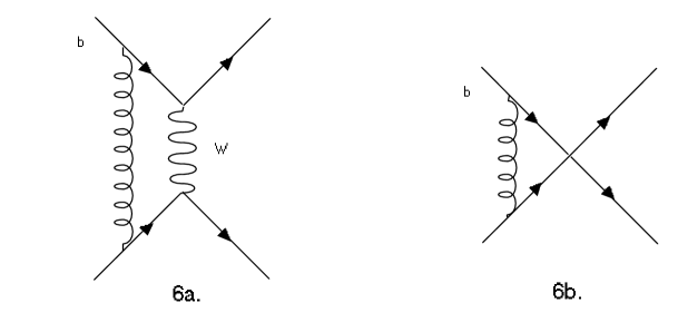
Figure 6: One loop correction to heavy quark decay.

This correction is finite and contains a large log of the form

$$\textrm{Diag. 6a}=\lambda_{1}\frac{\alpha_{s}(\mu)}{4\pi}\ln(m_{W}^{2}/m_{b}^{2}),$$ (29)

The diagrams which do not traverse the $W$ propagator do not contribute large logs and will not be of interest to us. If we are to save perturbation theory we must resum these logs. Indeed, the perturbative series for a generic Greens function of a theory which contains a large disparity of scales whose ratio is $\delta$, will contain the series

$$G_{log}=\sum_{n=1}^{\infty}(\frac{\alpha_{s}}{4\pi})^{n}\sum_{m=0}^{n}C_{m}^{(n)}\ln(\delta)^{m}.$$ (30)

If we take $(\frac{\alpha_{s}}{4\pi}\ln(\delta))$ to be order one, then we must resum all terms of the form $(\frac{\alpha_{s}}{4\pi}\ln(\delta))^{n}$. This is called the “leading log (LL)” approximation. This resummation as well as the “next to leading log (NLL) ($(\frac{\alpha_{s}}{4\pi}\ln(\delta))^{n-1}$)” and so forth are easily performed once we work within the framework of EFT.

The way EFT makes the resummation of the logs simple is by converting the problem to one with which we are more familiar. We know how to sum logs arising from UV divergences using the renormalization group (RG), so all we need to do is to figure out how to relate the logs in (30) to RG logs. The logs in (30) can be thought of as IR logs in the $m_{b}$ goes to zero limit, or UV logs if we take $M_{W}$ to infinity. But this second limit is exactly the limit we take in constructing the EFT. In the four-Fermi theory $M_{W}$ is taken formally to infinity, usually keeping only the first non-trivial term in the $1/M_{W}$ expansion. Let us see how the four Fermi theory reproduces the log in (29). The loop correction in the effective theory corresponding to those in figure 6a is shown in figure 6b, and is given by

$$\textrm{Figure 6b}=\lambda_{1}\frac{\alpha_{s}(\mu)}{4\pi}\left(\frac{1}{\bar{\epsilon}}-\ln(m_{b}^{2}/\mu^{2})\right)+\kappa.$$ (31)

Note that without doing any calculation we could have guessed the coefficient of the log in the effective theory from the full theory result. Since, as we discussed in the context of our toy model, the effective theory must reproduce the IR physics of the full theory, so the logs of $m_{b}$ must be identical in both theories. Using this result we may match onto the effective theory. The Wilson coefficient of the four-Fermi operator is

$$C_{4F}(\mu)=G_{F}\left(1+\lambda_{1}\frac{\alpha_{s}(\mu)}{4\pi}\left(\ln(M_{W}^{2}/m_{b}^{2})+\ln(m_{b}^{2}/\mu^{2})+\rho\right)\right)$$ (32)

Notice that we work in a mass independent prescription (usually $\overline{MS})$ where we subtract only the pole and possibly some dimensionless constants. Thus, the constant in (32) is scheme dependent. However, this scheme dependence is order $O(\alpha)$, which is sub-leading in the LL approximation. To cancel this $O(\alpha)$ scheme dependence we would need to go to the NLL, where the shift in the two loop anomalous dimension, generated by shifting schemes, will account for the change in the matching coefficient. Details of higher order calculations can be found in buras .

Exercise 1.5 Prove that the anomalous dimension is scheme independent only up to one loop. Also show that the beta function is scheme independent up to two loops. Assume that the coupling in the new scheme is analytic in the coupling in the old scheme, that is $g\prime(g)=a_{1}g+a_{2}g^{2}+.~{}.~{}.~{}$

Now in order to match we must make sure that series for $C_{4F}$ is converging. Thus we should choose $\mu$ to be order $M_{W}$, in which case $C_{4F}=G_{F}(1+\lambda_{1}\frac{\alpha_{s}(\mu)}{4\pi}\rho)$. In making this choice we have removed the large log from the matching, but if we are not careful the logs can still reappear. To see this we must consider the observable of interest. Using the optical theorem we may write the $B$ meson decay rate as MW

$$\Gamma=Im\int d^{4}x\frac{i}{m_{B}}\mid C_{4F}(\mu)\mid^{2}\langle B\mid T(O_{4F}^{\dagger}(x)O_{4F}(0)\mid B\rangle_{\mu}.$$ (33)

Any $\mu$ dependence in the Wilson coefficient must be cancelled by the $\mu$ dependence of the matrix element. If we choose $\mu$ to be order $M_{W}$, then the matrix element will also be renormalized at this high scale. This would clearly be a blunder, since the physics responsible for the decay is all taking place at the scale $m_{b}$. This blunder will reprise the log, since it will now show up in the matrix element as $\ln(m_{b}/\mu)$. To truly vanquish the log we want to renormalize the four Fermi operator at the lower scale $m_{b}$. But we know how to do this. We use the fact that the bare operator, $O_{B}=ZO_{R}$, where $Z$ includes both the operator and wave function renormalization, is $\mu$ independent

$$\left(\mu\frac{\partial}{\partial\mu}+\beta(g)\frac{\partial}{\partial g}+\gamma_{O_{4F}}\right)O_{4F}^{R}=0,$$ (34)

then since $Z=Z_{q}^{2}/Z_{O_{4F}}$

$$\gamma_{O_{4F}}=\mu\frac{\partial}{\partial\mu}\left(-\delta_{O_{4F}}+4\times\frac{1}{2}\delta_{2}\right)$$ (35)

Where $\delta_{O_{4F}}=-\frac{1}{\epsilon}\lambda_{1}\frac{\alpha_{s}}{4\pi}$ is the counter-term necessary to renormalize the four Fermi operator, and $\delta_{2}$ is the fermionic wave function counter-term

$$\delta_{2}=\frac{4}{3}\frac{\alpha}{4\pi}\frac{1}{\epsilon}.$$ (36)

The solution to the RG equation for $O_{4f}^{R}$ is

$$O_{4f}^{R}(\mu)=O_{4f}^{R}(\mu_{0})\exp\left(\int^{g(\mu)}_{g(\mu_{0})}\frac{dg}{g}\frac{\gamma_{O_{4F}}(g)}{\beta(g)}\right),$$ (37)

leaving

$$O_{4F}(m_{W})=O_{4F}(m_{b})\left[\frac{\ln(m_{W}^{2}/\Lambda^{2})}{\ln(m_{b}^{2}/\Lambda^{2})}\right]^{(A_{1}/(2b_{0}))},$$ (38)

where $b_{0}$ is the leading order beta function coefficient $11-2/3n_{f}$, and $\gamma_{O_{4F}}=\frac{\alpha_{s}}{4\pi}(A_{1}=2\lambda_{1}-\frac{16}{3})$. We are now free to evaluate the time order product, renormalized at the low scale $m_{b}$ without fear of generating large logs. Note that we can not claim to be accurate at order $\alpha_{s}$. We can achieve this level of accuracy only if we run at two loops. Since at order $\alpha_{s}$ we must keep all terms of the form $\frac{\alpha_{s}}{4\pi}^{n}\ln(\delta)^{n-1}$. Thus keeping the constant in the matching really bought us nothing. The systematics follow the rule that to achieve accuracy at order $\alpha^{n}$, you must match at order $\alpha^{n}$ and run at order $n+1$.

We have successfully removed that large and irrelevant scale $M_{W}$ from our calculation. Doing so enabled us to easily sum the large logs. But we are not quite done removing scales. In the decay process itself there are two relevant scales, namely $m_{Q}$ and $\Lambda_{QCD}$, the scale of hadronic physics. So we would expect that in our matrix elements we could induce logs of the ratio of these scales. But this is not a large log, so should we bother integrating out the scale $m_{Q}$? The answer is, of course, yes. Because if you recall in the introduction to this section we said that effective field theories do much more than just sum logs. They make approximate symmetries manifest.

Just as the scale $M_{W}$ was irrelevant for the decay process, so is $m_{Q}$. Since $m_{Q}\gg\Lambda_{QCD}$, the quark effectively acts as a static color source. As far as the light degrees of freedom are concerned, the heavy quark is a brick wall. If you increased its mass, the effects on the bound state would be essentially nil. Thus in the limit where the quark mass is taken to infinity, a new symmetry flavor symmetry emerges. If we have more than one quark with $m_{Q}\gg\Lambda$, then to leading order in $\Lambda/m_{Q}$, the quark decay is flavor independent. Furthermore, the spin of the heavy quark should decouple since the color magnetic dipole moment scales inversely with the mass, so we would expect the emergence of a spin symmetry as well in the large mass limit.

I.6 Heavy Quark Effective Theory

In this section I will briefly introduce HQET. I wont go into detail as this is now textbook material MW . But some of the concepts inherent in this theory will be necessary for the second lecture, so I will briefly recap the highlights and refer the reader to MW for more details.

What we would like to do is eliminate the scale $m_{Q}$ from the theory. However, we obviously need to keep the heavy quark field in the theory, so how do we keep the field and lose the mass? We begin by studying the dynamics of a heavy meson decay. As I said above the heavy quark should be static up to corrections of order $\Lambda/m_{Q}$. We may write the heavy quark momentum as

$$p_{Q}^{\mu}=m_{q}v^{\mu}+k_{\mu}~{},$$ (39)

where $v^{\mu}$ is the quarks’ 4-velocity ($(1,\vec{0})$ in the rest frame) and $k^{\mu}$ is what’s known as the “residual momentum” which is of order $\Lambda$. By studying the propagation of a heavy quark in a hadronic environment, It is easy to illustrate that the heavy quarks only role is to be a static color source Consider a heavy quark sitting inside a hadron being constantly bombarded by “soft” gluons(i.e. gluons with momentum of order $\Lambda$), as shown in figure (7). In the large mass limit we may simplify the intermediate propagators as follows

$$\frac{\gamma_{\mu}(m_{Q}v\!\!\!/+k\!\!\!/+m_{Q})\gamma_{\nu}}{(m_{Q}v+k)^{2}-m_{Q}^{2}}\approx\frac{\gamma_{\mu}(1+v\!\!\!/)\gamma_{\nu}}{2v\cdot k}+~{}O(k/m_{Q}),$$ (40)

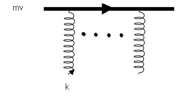
Figure 7: Scattering of a heavy quark off of gluons with momenta of order $\Lambda$.

so that the dependence on the heavy quark mass has disappeared. We expect the mass only to appear at sub-leading order in the mass expansion, and in phase space integrals. Furthermore, we also have

$$v\!\!\!/u(b)=u(b)+~{}O(k/m_{Q})$$ (41)

so we may make the replacement $\gamma_{\mu}\rightarrow v_{\mu}$ and the spin structure becomes trivial. In the real world where we have effectively two heavy quarks with $m_{Q}\gg\Lambda$, charm and bottom, we can see that in the large mass limit we should generate an $SU(2)_{flavor}\times SU(2)_{spin}$ symmetry, and this symmetry should be manifest in our effective theory.

We can determine the action for the effective field theory by matching. We consider the full theory propagator, again splitting the momentum into a large and small pieces, and expand in the residual momentum

$$G^{(2)}(p)=\frac{i}{m_{Q}v\!\!\!/+k\!\!\!/-m_{Q}+i\epsilon}\approx\frac{i(1+v\!\!\!/)}{2v\cdot k+i\epsilon}.$$ (42)

Now we need to find an action which has the proper quadratic piece to reproduce this two point function. We do this in two steps: First we notice that the numerator of the effective propagator is a projector onto the large components of the heavy quark spinor. So we should split up the heavy quark spinor into “large” and “small” components. Then, to remove the heavy quark mass yet retain the field itself, we simply extract the mass dependence via a field redefinition GeorgiII ,

$$q(x)=e^{-imv\cdot x}\left(h_{v}(x)+H_{v}(x)\right),$$ (43)

where

$$h_{v}(x) = e^{imv\cdot x}\frac{1}{2}(1+v\!\!\!/)q(x)$$

$$H_{v}(x) = e^{imv\cdot x}\frac{1}{2}(1-v\!\!\!/)q(x).$$ (44)

Here is where HQET differs from the usual effective theories where we remove entire fields from the action. The fields have labels $v$. A field with a label $v$, destroys a particle whose four momentum is fixed to be within $\Lambda$ of $mv_{\mu}$. That is, the field itself only has Fourier components less than $\Lambda$. This is in accordance with our physical expectations. Once we integrated out the hard modes, the only modes left have momenta of order $\Lambda$ whose effect is only to jiggle the heavy quark. So we write the momentum of the heavy quark as $p=m_{Q}v+k$, where $k$ is called the “residual momentum” and is of order $\Lambda$. Thus, derivatives acting on this rescaled field are of order $\Lambda$.

We may now substitute this parameterization of the full QCD field into the Lagrangian to arrive at

$${\it L}_{QCD}=\bar{q}(iD\!\!\!/-m_{Q})q~{}=~{}\sum_{v}\bar{h}_{v}(iv\cdot D)h_{v}~{}+~{}O\left(\frac{\Lambda}{m_{Q}}\right).$$ (45)

Notice the sum over velocities. It is needed because we should allow for arbitrary four velocities of the heavy quark, and remember that once we fix a label the momentum is fixed up to some small an amount of $O(\Lambda)$. Technically, this means that there is a super-selection rule, which is defined by the statement that states with four-velocities which differ by more than $\Lambda$ exist in different Hilbert spaces. So to allow for differing velocities we have to “integrate in” the different sectors. If we are only interested in processes with no weak decays this point becomes moot since we can go to a frame where the heavy quark is static. However, if we want to look at for instance a $b$ to $c$ transition then a large ”external” momentum is injected which drastically changes the velocity of the heavy quark. In the effective theory this is described by the flavor changing current, whose labels reflect the connection between different Hilbert spaces

$$J(x)=\sum_{v,v^{\prime}}~{}\bar{h}^{c}_{v}~{}\Gamma~{}h_{v^{\prime}}^{b}(x)$$ (46)

These type of label changing operators will play an important role in the next lecture.

We performed a Taylor expansion of our tree level propagator, should we expect this replacement to work even in loop diagrams? The answer is of course, yes, and the reason is (not to flog a dead horse) that the part of the loop integral for which the Taylor expansion is ill suited comes from UV physics, which is local and can always be absorbed into counter terms. Technically, this can be see in a simple fashion. Take any full theory integral, $I$ and write it as

$$I=(I-I_{EFT})+I_{EFT}$$ (47)

If $I$ is finite, then Taylor expanding and integrating commute and there is no work to be done, the EFT will reproduce the full theory to any desired order in the inverse mass. If the integral diverges, then all we need to do is differentiate it enough times with respect to the external momentum to make it finite and then perform the Taylor expansion. The value of the full integral will differ from the expanded integral by some polynomial in the external momentum, i.e. a counter-term. Using this type of argument inductively an all orders proof has been provided both for four Fermi theory WittenEFT and HQET Grinstein . HQET is particularly simple because there is only one relevant IR region, $k\sim\Lambda_{QCD}$. So we expect that Taylor expanding around small loop momenta will correctly reproduce the IR physics. Other theories may have more relevant IR momentum regions as will be discussed later on in these lectures.

I.7 The Method of Regions

This line of reasoning can greatly simplify matching calculations. Suppose we wish to match onto to HQET at one loop. The standard recipe is, take the full theory result, expanded in powers of $k/m_{Q}$, and subtract the value of the corresponding effective theory result . But there is actually a way to make life a lot less complicated by utilizing some of the magic of dimensional regularization and asymptotic expansionsAE . Instead of first calculating in the full theory and then expanding, one can Taylor expand at the level of the integrand, assuming that the loop integrals are dominated by momenta much larger than the external momenta. By working in this way we will miss out on non-analytic pieces, but that’s OK since we know that they cancel in the matching. How do we know that this method correctly reproduces the matching coefficient? One way to think about it is in terms of the “method of regions”MoR . The idea is that in dimensional regularization the integral will receive contributions from momenta of order the heavy quark mass (“hard modes”) as well as momenta of order the residual momenta (“soft modes”). This is true even for divergent integrals since the contribution from modes much larger than the quark mass lead to scaleless integrals which vanish. Let us see how this works in a simple one loop example. Consider the two point function integral

$$I=\int\frac{d^{n}q}{(2\pi)^{n}}\frac{1}{(q^{2}+i\epsilon)}\frac{1}{((p_{Q}+k-q)^{2}-m_{Q}^{2}+i\epsilon)},$$ (48)

$k$ is the residual momentum of order $\Lambda_{QCD}$. To extract the hard contribution we assume $q$ is of order $m_{Q}$ and Taylor expand the integrand up to order $1/m_{Q}$

$$I_{h}=\int\frac{d^{n}q}{(2\pi)^{n}}\frac{1}{(q^{2}+i\epsilon)}\frac{1}{(q^{2}-2p\cdot q+i\epsilon)}(1-\frac{2(p-q)\cdot k)}{q^{2}-2p\cdot q+i\epsilon}).$$ (49)

Whereas the soft part of the integral is found by assuming the loop momentum is order $k$. Keeping only the leading order piece in this region we find

$$I_{s}=\int\frac{d^{n}q}{(2\pi)^{n}}\frac{1}{(q^{2}+i\epsilon)}\frac{1}{2p\cdot(k-q)+i\epsilon},$$ (50)

which is exactly the HQET contribution. So if we can show that the sum of these two contributions is equal to $I$, then we’ve shown that the hard piece is exactly what we would call the matching. The full integral can be performed using text-book methods

$$I=\frac{i}{16\pi^{2}}\left(\frac{1}{\bar{\epsilon}}-\ln(\frac{m_{q}^{2}}{\mu^{2}})+2+\left(\frac{1}{\hat{p}^{2}}-1\right)\ln(1-\hat{p}^{2})\right),$$ (51)

where $\hat{p}^{2}=1+\frac{2p_{Q}\cdot k}{m_{Q}^{2}}$. The hard piece is given by

$$I_{h}=\frac{i}{16\pi^{2}}\left(\frac{1}{\bar{\epsilon}}+2-\ln(\frac{m_{Q}^{2}}{\mu^{2}})+\frac{k\cdot p_{q}}{m_{Q}^{2}}\left(-\frac{1}{\bar{\epsilon}}+\ln\frac{m_{Q}^{2}}{\mu^{2}}-2\right)\right)$$ (52)

The soft integral has denominators of differing dimensions, so it’s helpful to use the identity

$$\frac{1}{a^{n}b^{m}}=2^{n}\frac{\Gamma[n+m]}{\Gamma[n]\Gamma[m]}\int_{0}^{\infty}d\lambda\frac{\lambda^{m-1}}{(a+2b\lambda)^{n+m}}.$$ (53)

Then following standard techniques we arrive at

$$I_{s}=\frac{i}{16\pi^{2}}\frac{k\cdot p_{q}}{m_{Q}^{2}}\left(\frac{1}{\bar{\epsilon}}+2-2\ln(\frac{-2v\cdot k}{\mu})\right).$$ (54)

Expanding the full theory result (51) and comparing it to the sum of (54) and (52), we find agreement between the two. Notice that both $I_{h}$ and $I_{s}$ have spurious divergences which cancel each other. For more complicated theories, such as $NRQCD$, there are more regions to worry about, and one must be sure that they are all accounted for in order to correctly reproduce the full theory result. Furthermore, one must be careful when matching at two loops using the above trick. Doing so would necessitate keeping $\epsilon$ dependence in the effective theory actionBSS ; MSI .

Exercise 1.6 In the last example I have expanded in $\epsilon$ before expanding in $1/m_{q}$. Show that the equality holds true even if you don’t expand in $\epsilon$ by calculating the full result exactly and then expanding in $1/m_{Q}$.

The method of “Asymptotic Expansions” has been proven to work to all orders for both the large momentum and large mass limits for Euclidean momenta. However, there are no known counter-examples to two loops in Minkowski space.

I.8 A Caveat About Scaleless Integrals

Suppose we chose to match exactly at zero external momentum. We are free to do this if we are not interested in corrections which are sub-leading $p$. It is often the case that at this point the integrals in the effective theory will be scaleless and thus vanish (this is true in HQET as well as NRQCD). However, this does not mean that we can conclude that the effective theory operator under consideration has no anomalous dimension. To calculate the running in the effective theory we need to account for the fact that the scaleless integral $I_{EFT}$ is giving zero because of a cancellation

$$I_{EFT}=C~{}(\frac{1}{\epsilon_{UV}}-\frac{1}{\epsilon_{IR}}).$$ (55)

Given any logarithmically divergent scaleless integral we can always perform this split algebraically

$$\int{d^{d}k\over{(2\pi)^{d}}}\frac{1}{k^{4}} = \int\frac{d^{d}k}{(2\pi)^{2}}\left(\frac{1}{(k^{2})(k^{2}-m^{2})}-\frac{m^{2}}{(k^{4})(k^{2}-m^{2})}\right)$$ (56)

$$= \frac{i}{16\pi^{2}}\left(\frac{1}{\epsilon_{UV}}-\frac{1}{\epsilon_{IR}}\right).$$

However, if and only if, we know that the full theory has no IR poles, can we correctly conclude that the anomalous dimension in the effective theory vanishes when we have scaleless integrals. When the full theory has no IR poles, the effective theory has no IR poles and since in the effective theory (for scaleless integrals) there is also a one to one correspondence of UV and IR poles we may conclude that the effective theory has no UV poles. This is an important point: We can’t ignore dimensionless integrals in dimensional regularization in the effective theory unless we are sure that we have correctly accounted for all of the IR poles in the full theory.

I.9 Power Counting

In most effective field theories the power counting is as simple as keeping track of powers of the mass. However, this will no longer be true in more complicated EFTs. Power counting is trivial in HQET, but I want to go through it pedantically, since such an analysis will bear fruit later. Once we’ve removed the heavy quark mass, there is only one relevant scale, $\Lambda$. All of the fields have support only over regions of order $1/\Lambda$ so we should expect that dimensional analysis will yield the correct power counting. Let’s see if this is true. The leading order action,

$$S^{HQET}=\int d^{4}x~{}\sum_{v}\bar{h}_{v}(iv\cdot D)h_{v},$$ (57)

should scale as $O(1)$. Each field scales as $\Lambda^{3/2}$ while the derivative scales as $\Lambda$. Finally, since the fields only have support over region of size $\Lambda$, $d^{4}x\propto\Lambda^{-4}$, the leading order action does indeed scale properly. In general, there may be more than one scale involved and the scaling of the fields is instead fixed according to the leading order action. All other operators in the action should scale as positive powers of $\Lambda$, since if there were operators with negative powers, power counting will be jeopardized.

I.10 The End of Our Calculation

We now have all the ingredients to finish our inclusive B decay calculation. We started with a theory with three scales, $M_{W}$, $m_{b}$ and $\Lambda$. We eliminated $M_{W}$, ran down to $m_{b}$ and are now have the power, via $HQET$, to remove $m_{b}$. Removing this scale is crucial, even if we are not interested in the enhanced symmetry. To see this, we have to figure out how to evaluate the time ordered product (33). I will only sketch this final part of the calculation since it’s is explained in details in MW . The main point is that the non-local operator product can be simplified using an operator product expansion (OPE) much as in deep inelastic scattering (DIS) DIS (though the use of the OPE in the present context is not rigorously justified as it is in DIS). The TOP can be expanded into a set of local operators, schematically

$$\int d^{4}xe^{-iq\cdot x}O(x)O(0)\simeq C_{1}(q^{2},\mu)+C_{2}(q^{2},\mu)\frac{O_{2}(\mu)}{q^{2}}+C_{3}(q^{2},\mu)\frac{O_{3}(\mu)}{q^{4}}+.~{}.~{}.$$ (58)

where $q$ here is the large scale in the process (for us $q\sim m_{b}$). The utility of the expansion is predicated on our ability to truncate it. As long as when we take the matrix elements of the $RHS$, we don’t introduce a scale of order $q$ upstairs, we can safely ignore terms of higher order in $1/q^{2}$. Now we can see that in the case of $B$ decays we will run into exactly this problem since we will be taking matrix elements between $B$ states. So that while each term in the expansion may be down by powers of $q$, i.e. $m_{b}$, taking the matrix element will generate expectation values which scale with positive powers of $m_{b}$. The solution to this problem is simply to go to the effective theory, where the scale $m_{b}$ is gone and all matrix elements scale only as $\Lambda$. How the OPE is performed in HQET is discussed in MW .

I.11 EFT and $\overline{MS}$

I want to emphasize the fact that using a mass independent prescription is crucial for this, as well as most other, EFT calculations. In fact, EFT and mass independent prescriptions go usually go hand in hand (lattice effective theories are exceptions to this rule). To see the need for this marriage, suppose we’re trying to calculate the running of a gauge coupling. Our prescription can not affect any physical prediction, but a poor choice of prescription can lead to an ill behaved perturbative series. Let’s compare and contrast the contributions of a massive fermion to the QED vacuum polarization in the $\overline{MS}$ and momentum subtraction $(ms)$ schemes.

$$\Pi_{\mu\nu}^{\overline{MS}}=\frac{-ie^{2}}{2\pi^{2}}(p_{\mu}p_{\nu}-p^{2}g_{\mu\nu})\int_{0}^{1}dx~{}x(1-x)\ln\left[\frac{m^{2}-p^{2}x(1-x)}{\mu^{2}}\right],$$ (59)

$$\Pi_{\mu\nu}^{{ms}}=\frac{-ie^{2}}{2\pi^{2}}(p_{\mu}p_{\nu}-p^{2}g_{\mu\nu})\int_{0}^{1}dx~{}x(1-x)\ln\left[\frac{m^{2}-p^{2}x(1-x)}{m^{2}+M^{2}x(1-x)}\right],$$ (60)

where $M$ is the scale at which we have chosen to define the coupling, so that in the $ms$ scheme $\Pi(-M^{2})=0$. For $p^{2}\ll m^{2}$ we may choose $\mu,M\simeq m$ and neither scheme will produce large logs. The problem arises when we have two fermions with very disparate masses. Indeed, suppose that in addition to the fermion of mass $m$, we also a massless charged fermion in the theory. Then we can see that in the $\overline{MS}$ scheme, there is no choice of $\mu$ for which there are no large logs. On the other hand in the $(ms)$ scheme we can choose $M^{2}\simeq-p^{2}$ and no large logs will remain. The reason for this difference is that the $ms$ scheme is a “decoupling scheme” while $\overline{MS}$ is not. That is, in the $\overline{MS}$ massive particles do not decouple in the low energy limit. That is exactly why we should work in an EFT, where we remove the heavy particles by hand. This is the small price we have to pay in order the easily sum the logs. Indeed, in the $ms$ scheme we will need to calculate $\alpha_{s}(-M^{2})$, given its value at some other momenta at which it was measured $M_{0}$, and solving the RG equations in this scheme is more difficult. I should also say that even if you work in a mass independent scheme you don’t have to use an EFT, it’s just that without EFT calculations become more cumbersome since the low energy observables will receive contributions from all the heavy fields which re-introduce large logs. But in the end if you are careful you should always get the same result. Using an EFT will just make your life a lot easier.

I.12 The Force Law in Gauge Theories

When working in an effective theory, or any theory for that matter, it is easy to get confused if one does not work with physical quantities. Coupling are in general scheme dependent and have no physical meaning, thus it is always best to have in mind some measurable observable when doing a calculation. Often in these lectures instead of talking about measuring a coupling, I will instead talk about measuring the force between static sources. In this way we can be assured that our result is in no way ambiguous. This force or potential is intimately related to what we normally call the coupling, but is a measurable quantity and thus scheme independent.

We begin by showing that the static potential can be extracted by calculating the expectation value

$$Z[J]=\langle 0\mid T(e^{-ie\int d^{4}xej^{\mu}(x)A_{\mu}(x)}\mid 0\rangle$$ (61)

for a stationary charge distribution which turns off adiabatically at $\pm\infty$. then using standard arguments (see Peskin )

$$\lim_{T\rightarrow\infty}Z[J]\propto e^{iE(J)T},$$ (62)

where $E(J)$ is the vacuum energy in the presence of the source $J$. It is left to the reader to show that $Z[J]$ is nothing but the expectation value of the gauge invariant time-like Wilson loop

$$W(r,T)\equiv\langle 0\mid Tr\left(P(e^{\oint A_{\mu}dx^{\mu}})\right)\mid 0\rangle$$ (63)

where $P$ stands for path ordering.

For a free Abelian theory, i.e. no matter, things simplify tremendously since the action is quadratic in the gauge field, and hence the functional integral can be done exactly, resulting in

$$Z[J]\propto e^{-\frac{ie^{2}}{2}\int d^{4}xd^{4}yJ^{\mu}(x)\Delta_{\mu\nu}(x,y)J^{\nu}(y)}$$ (64)

where $\Delta_{\mu\nu}$ is the photon propagator. We will be interested in the energy of two static sources, of opposite charge, separated by a spatial distance $r$. So that

$$J_{\mu}(x)=e\delta_{\mu 0}\delta^{3}(\vec{x}-\vec{r})-e\delta_{\mu 0}\delta^{3}(\vec{x})$$ (65)

then it is straightforward to show that

$$E(r)=\frac{-e^{2}}{4\pi r}.$$ (66)

Diagrammatically, one can arrive at result by using Wicks’ theorem on (61). At leading order in the coupling there is one diagram corresponding to one photon exchange, resulting in the integral

$$I_{2}=\frac{1}{4\pi^{2}}\int\frac{dt_{1}dt_{2}}{(t_{1}-t_{2})^{2}-r^{2}}$$ (67)

At next order there are two Wick contractions, but these sum to give the square of $I_{2}$ with a combinatoric factor of $1/2$. One can then see that subsequent Wick contractions will just fill out the power series expansion of the exponentialFischler .

Now when we include matter, the only new diagrams which arise correspond to corrections to the photon propagator. Thus all the logarithmic corrections to Coulomb’s law will arise from loops in the photonic two point function. Resumming the vacuum polarization graphs results in the corrected form of the potential

$$E(r)=\frac{-e^{2}_{eff}(r)}{4\pi r}$$ (68)

where

$$e^{2}(r)_{eff}=\frac{e^{2}(\mu)}{(1+\frac{e^{2}(\mu)}{6\pi^{2}}\ln(r/\mu))}.$$ (69)

When we go to QCD, things get slightly more complicated but, at least up to two loops, the same reasoning goes through Fischler ; Kogut . The potential is given by the logarithmically corrected Coulomb potential with the appropriate beta function. However, at three loops one encounters an infra-red divergenceADM arising from the fact that there can be intermediate color octet states that live for long times. These colored states can interact with long wavelength gluons since they have non-vanishing dipole moments. However, this should not bother us. The vacuum matrix element contains long distance physics, and thus it need not be infra-red finite in perturbation theory.

II Lecture II: Non-Relativistic Effective Theories.

II.1 The Relevant Scales and the Free Action

In the previous lecture we displayed the utility of encapsulating the UV physics in an effective field theory. In our toy model we completely removed a heavy field, while in HQET we kept the field but removed the mass. In both of these cases the non-analytic momentum dependence came from rather simple kinematic configurations. In the toy model all the cuts were generated from intermediate light particles going on shell. In HQET the cuts come from either gluons or heavy quark lines going on shell with $k_{\mu}\simeq\Lambda$. But there are certain kinematic situations where the momenta configurations which determine the cuts of a Greens function can be more complicated. Consider for instance a non-relativistic bound state such as Hydrogen or quarkonia. In this case the on-shell external lines in our Greens functions will obey a non-relativistic dispersion relation, leading to the propagator

$$G^{(2)}(E,\vec{p})=\frac{i}{E-\frac{\vec{p}^{2}}{2m}+i\epsilon},$$ (70)

and the cuts will come from a momenta region where $E\simeq\frac{\vec{p}^{2}}{2m}$. Notice that, as opposed to the case of our toy model and HQET where there was only one relevant low energy scale, $m_{L}$ and $\Lambda$, respectively, a non-relativistic theory contains two scales namely $E\simeq mv^{2}$ and $p\simeq mv$. That is, the typical size of the bound state is the Bohr radius $r_{B}\simeq 1/(mv)$ and the typical time scale is the Rydberg $R\simeq 1/mv^{2}$. The existence of these two scales complicates matters. As in our previous cases we’d like to eliminate all the large scales from the theory, leaving a nice simple theory with only one low energy scale. Unfortunately, as we shall see this is not possible due to the fact that the two scales $mv$ and $mv^{2}$ are correlated, and must exist simultaneously.

Suppose we try to treat the scale $mv$ in the same way that we treated the mass in HQET, i.e. by rescaling the quark fields. This would indeed remove it from the theory, and all derivatives would scale homogeneously as $mv^{2}$. However, since spatial fluctuations on the scale $mv$ are crucial to the dynamics of the bound state, we know that this can’t be the end of the story as far as this scale is concerned. In fact, as we shall see, the Coulomb potential is built from the exchange of gluons with three momentum of order $mv$. So if we eliminate the modes with momenta of order $mv$ by re-phasing the field we had better figure out how to put (integrate) them back in. At first, this seems like a silly thing to do, but we will see that this formal manipulation will simplify the construction of the effective theory since all spatial derivatives will scale homogeneously. If we did not do this re-phasing we would not have manifest power counting, as we shall see.

But we are jumping the gun a little. Let us treat one scale at a time from top down. We begin by first eliminating the mass from theory as we did in HQET by a simple rescaling of the field

$$Q=e^{-im_{Q}t}(\psi+\chi),$$ (71)

where

$$\psi=e^{im_{Q}t}\frac{1}{2}(1+\gamma_{0})Q$$ (72)

$$\chi=e^{im_{Q}t}\frac{1}{2}(1-\gamma_{0})Q$$ (73)

are the large and small two spinors of the full Dirac quark spinor, respectively. As opposed to HQET, there is now a preferred frame, namely the center of mass frame. So we will assume that we are working in this frame from now on. Thus when we rescale the field we won’t sum over all four velocities, as we did in HQET. Also I won’t bother labelling the fields by their four velocity, as there is only one relevant label velocity $(1,\vec{0})$. If we wanted to allow for weak decays we would have to include a sum over four-momenta labels as we did in HQET.

Now we can separate the next largest scale, $mv$, from the other scales in the theory by writing

$$\psi=\sum_{\bf{\vec{p}}}e^{-i\vec{p}\cdot\vec{x}}\psi_{\bf{\vec{p}}}(x)$$ (74)

where the label on the field fixes the three momentum to be order $m\vec{v}$. Spatial derivatives acting on $\psi_{\bf{\vec{p}}}(x)$ are of order the residual three momenta $mv^{2}$. This way of splitting up momenta into a large label piece and a residual momentum is depicted in figure (8).

Figure 8: This diagram depicts how the momenta are divided by the labelling process. The largest label $v_{\mu}$ has been frozen to be $(1,0,0,0)$. The three momenta are split into a large label $\vec{p}$ of order $mv$, and a small residual momenta of order $mv^{2}$ depicted by the smallest boxes.

The free piece of the action can then be read off by substituting the expansions (71) and (74) into the full QCD action, solving for the small component $\chi$ in terms of the large component $\psi$, and keeping only the leading order terms in an expansion in the small parameter $v$,

$$L_{0}=\sum_{\bf{\vec{p}}}\psi^{\dagger}_{\bf{\vec{p}}}(i\partial_{0}-\frac{\bf{\vec{p}}^{2}}{2m})\psi_{\bf{\vec{p}}}~{}+~{}(\psi\rightarrow\zeta).$$ (75)

Notice that we have dropped all spatial derivative terms, such as ${\bf\vec{p}}\cdot\vec{\partial}$, as they are higher order in $v$. Remember that the $\bf{\vec{p}}$ which appears in the action is a C number and not an operator. $\zeta$ is the large component of the anti-quark field, which arises when we re-phase with the opposite sign in (60), and its action on the Fock space is to destroy an anti-quark.

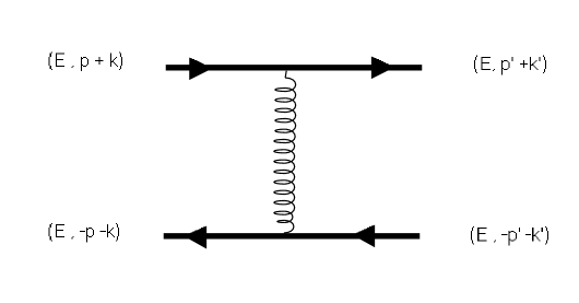
Figure 9: Full theory matching which generates the Coulomb interaction. The momenta are split up into a large piece ($\vec{p}$) which is order $mv$ and a residual piece $k$ which is of order $mv^{2}$. The large piece corresponds to the label of the field.

II.2 Interactions

The interactions can be fixed by a matching calculations, though some interactions are more simply read off by gauge invariance, as we shall see. Let’s start by considering the t-channel exchange of a gluon between a quark and anti-quark in the full theory as shown in figure (9). Since the initial and final state quarks are on shell, the gluon momentum must scale as $(mv^{2},mv)$. We split the external three momenta into a piece of order $mv$, corresponding to the label of the field, and a residual momenta $k$, which if of order $mv^{2}$. We then expand the full theory result in $v$ and write the full theory spinors in terms of the two spinors (72). The leading order piece generates the operator

$$L_{C}=g^{2}\sum_{\bf{\vec{p}}_{i}}\psi^{\dagger}_{\bf{\vec{p}}^{\prime}}T^{a}\psi_{{\bf\vec{p}}}\frac{1}{(\bf{\vec{p}}-\bf{\vec{p}}^{\prime})^{2}}\zeta^{\dagger}_{-\bf{\vec{p}}^{\prime}}\overline{T}^{a}\zeta_{-\bf{\vec{p}}}$$ (76)

This operator is nothing but the Coulomb potential. It is called a “potential” because the interaction is non-local in space but instantaneous in time. Notice that $L_{C}$ includes a sum over all possible labels. This is in stark contrast to HQET where an external current is needed to change labels. Here in NRQCD, there are terms in the action which themselves change labels. What we have done seems a little perverse at first. We have integrated out modes (via a field rescaling) only to integrate them back in by summing over labels. However, we will see that there is a method to the madness.

Now let us power count to see if the operator (76) we matched onto should appear in the leading order Lagrangian. To do so we first need to determine how the fields scale. The easiest way to do this is to use the fact that the kinetic piece should be order one in our power counting. So, following the line of reasoning developed in section I.9, we first power count the measure in the action. The quark field has support over $1/v^{2}$ in the time direction and order $1/v$ in the spatial directions so we conclude that $d^{4}x\sim v^{-5}$ and $\psi\sim v^{3/2}$. In this way the kinetic piece (75) scales as $v^{0}$. Now let us consider the operator (76). The measure again scales the same way as in the kinetic piece since the operator contains only heavy quarks, so that

$$O_{C}\sim v^{-5}(v^{3/2})^{4}v^{-2}\sim v^{-1}.$$ (77)

Thus $O_{C}$ certainly should be treated as a leading order piece in the Lagrangian. Indeed, the fact that it actually is enhanced relative to kinetic piece is worrisome as it could lead us to the conclusion that there is no sensible $v\rightarrow 0$ limit, which is the limit in which the leading order action is exact. We will come back to this issue later. For now we will conclude that the Coulomb potential will have to be treated non-perturbatively in our theory. The operator can be interpreted in terms of the exchange of a non-propagating Coulomb gluon. If we wish we can re-write this operator in terms of an auxiliary field (i.e. a field without a kinetic term)LS

$$L_{c}=\sum-g(\psi^{\dagger}_{\vec{\bf{p}}}\psi_{\vec{\bf{p}^{\prime}}}+\chi^{\dagger}_{\vec{\bf{p}}}\chi_{\vec{\bf{p}^{\prime}}})A_{0_{\vec{\bf{p}}^{\prime\prime}}}+{1\over 2}(\vec{\bf{\nabla}}A_{0_{\vec{\bf{p}}}})^{2}.$$ (78)

Writing things in this way will make our relevant degrees of freedom more explicit when we discuss NRQCD in terms of the method of regions as discussed in (I.7). But this is just a formal manipulation. In general, “off shell” modes will not appear in the Lagrangian.

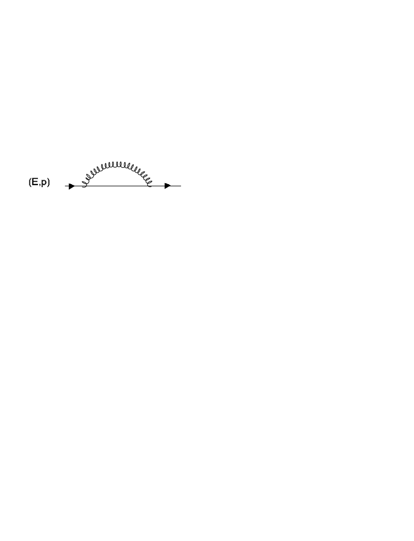
Figure 10: Self energy diagram is NRQCD. The labelling technique automatically implements the dipole expansion.

II.3 The Multipole Expansion and Ultra-Soft Modes

What interactions are there in the one quark sector? We should allow for all interactions which leave the fields on-shell to within order $mv^{2}$, which is the scale of their residual momentum, as these modes will certainly generate non-analyticity in our amplitudes. One obvious interaction we can have is of the usual form $\psi^{\dagger}A\psi$, if $A$ is a gluon which carries momentum scaling as $(mv^{2},mv^{2})$. In fact, gauge invariance seems to lead us to this type of interaction, since we would expect that the $\partial_{0}$ in (75) should be elevated to a covariant derivative. Let’s see if this new interaction does indeed to correspond to $(mv^{2},mv^{2})$ gluons. The self energy diagram in figure (10) is given by

$$i\Sigma=g_{s}^{2}C_{F}\int{d^{d}g\over{(2\pi)^{d}}}\frac{1}{(g^{2}+i\epsilon)}\frac{1}{(E-g_{0}-\frac{\bf{\vec{p}^{2}}}{2m}+i\epsilon)}.$$ (79)

Now we will show that the gluon running through the loop does have momentum which scales as $(mv^{2},mv^{2})$. The important point to note here is that the fermion propagator does not carry any of the three momentum of the gluon. The $\bf{\vec{p}}^{2}$ piece is just the label of the external line. This is an implementation of a dipole expansion Labelle ; GR

$$A^{a}_{0}(t,{\bf{\vec{x}}})=A^{a}_{0}(t,{\bf{\vec{0}}})+{\bf{\vec{x}}\cdot\vec{\nabla}}A^{a}_{0}(t,\bf{\vec{0}})+.~{}.~{}.~{}$$ (80)

Exercise 2.1 Working with a coordinate space dipole expanded Lagrangian reproduce equation (79) for the self-energy.

It is interesting that the act of separating the scales via the re-labelling technique has automatically generated a dipole expansion. This demonstrates a persistent fact in effective field theories. If you have properly separated the scales, then each diagram in the effective theory should scale homogeneously in the expansion parameter. In order for this to be true any given integral should be dominated by just one region of momenta. Let us see how this happens in our self-energy diagram. Doing the integral by contours we see that the $g_{0}\sim\mid{\bf{\vec{g}}}\mid\sim mv^{2}$, there are no other relevant regions. Note that if we had not dipole expanded then the integral would have received a contribution where $g$ was of order $m$, and the integral would not scale homogeneously in $v$. This would spoil the power counting in the theory GR . Gluons which have momenta of order $(mv^{2},mv^{2})$ are called “Ultra-Soft (US)”, and are on shell-modes which have the usual $F^{2}$ kinetic term in the Lagrangian. These modes are sometimes also referred to as “radiation” or“dynamical” gluons which can be thought of as contributing to higher Fock states in the onia. Note, however, that the $A_{0}$ US mode can be eliminated from the leading order action by redefining the quark field in the following fashion

$$\psi^{\prime}(x)=Pe^{ig\int_{-\infty}^{t}A_{0}(n_{\mu}\lambda+{\bf\vec{x}})d\lambda}\psi(x),$$ (81)

where P stands for path ordering and $n_{\mu}$ is the time like unit vector $(1,\vec{0})$. The $A_{0}$ US gluons will then reappear in the action at higher order in $v$. Thus without doing any calculations we can conclude that the interactions due to $A_{0}$ US modes must vanish at leading order.

There are additional US spatially polarized gluons ($\vec{A}$) which play an important role at sub-leading order in $v$. We can determine the coupling of these gluons in a very simple way using what is known as reparameterization invarianceML (RPI). The idea behind RPI is quite simple, yet its ramifications are powerful. The point is that when we pulled out the three momenta from the heavy quark field, there was an ambiguity . We could just as easily rescaled by $e^{(}{imv+k})$ where $k$ is order $mv^{2}$. Thus our action should be independent under small shifts in the label. This just means that every time we see a ${\bf\vec{p}}$ it should be accompanied by a ${\bf\vec{\partial}}$. Then by gauge invariance we know that we should make the replacement

$${\bf\vec{p}}\rightarrow{\bf\vec{p}}+i{\bf\vec{D}}.$$ (82)

everywhere we see ${\bf\vec{p}}$. Notice that this form has to hold to all order in perturbation theory. This is quite a useful piece of information, as it tells us that many operators in our action will have vanishing anomalous dimension.

The net effect of this substitution is the generation of subleading terms in the dipole expansion (80). For instance, the kinetic term ${\bf\vec{p}^{2}}/(2m)$ will generate the subleading dipole interaction $\psi^{\dagger}({\bf\vec{p}\cdot\vec{A}}/m)\psi$. Note that ${\bf{\vec{D}}}=\vec{\partial}-ig\vec{A}$, scales as $v^{2}$, since when the derivative acts on the heavy quark field it brings down a factor of the residual momentum which is of order $v^{2}$, and, as you can prove for yourself, the ultra-soft gluon field scales as $v^{2}$ as well.

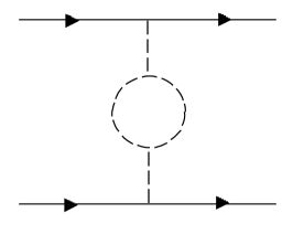
Figure 11: A graph which one might have hoped would induce a running potential, which does not exist in the effective theory.

II.4 Soft Modes

So now we have shown that there are two types of gluonic modes which contribute to the non-analytic behavior of the low energy theory: potential gluons (which are not dynamical), whose momenta scale as $(mv^{2},mv)$, and “ultra-soft” (US) gluons whose momenta scale as ($mv^{2},mv^{2})$. But this can not be the end of the story. In particular, we know that the Coulomb potential should run even once we are below the scale $m$, due to the non-Abelian nature of the theory. We might expect that a diagram such as (11) could account for the running of the coupling/potential. However, this diagram does not exist in the effective theory, since the Coulomb gluon is not a propagating degree of freedom (it is simple to show that this diagram vanishes). The Coulomb gluon sometimes called an “off-shell” mode because it can never satisfy the gluon dispersion relation $g_{0}^{2}={\bf\vec{g}}^{2}$, and thus never appears as an external state. To generate a running Coulomb potential we must include a new set of propagating degrees of freedomMoR ; Griesshammer , namely, “soft gluons”, whose momenta scale as $(mv,mv)$.

How could such degrees of freedom interact with the heavy quarks? We notice that because their energy scales as $mv$, any such interaction would throw the heavy quark off-shell by an amount of order $mv$. So we know that we need at least two interactions. The simplest such interactions are shown in figure (12).

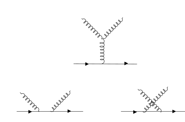
Figure 12: Leading order matching graphs between heavy quarks and “soft” gluonic modes with momenta of order $(mv,mv)$. Not shown are the similar diagrams with ghost fields,

Now since these modes have a “large” component, in both their energy and momentum, we need to rescale the field so that all derivatives acting on the field scale as the lowest scale in the theory, $mv^{2}$. So as in the case of the heavy quark field we write

$$A^{a}_{\mu}(x)=\sum_{q}e^{-iq\cdot x}A^{a}_{q\mu}(x).$$ (83)

Notice the field is now labelled by a four momentum. Now we match the Compton graphs in figure (12) onto the effective theory. To do so we split the external momenta of the gluon fields into a label piece and a small residual momentum

$$Q_{\mu}=q_{\mu}+k_{\mu}~{},$$ (84)

and expand the diagram in powers of $v$. Keeping only the leading order result we find

$$L_{soft}^{int} = -4\pi\alpha_{s}\sum_{q,q^{\prime}\mathbf{p},p^{\prime}}\Biggl{\{}{1\over q^{0}}\psi_{\bf{\vec{p}^{\prime}}}^{\dagger}\left[A^{0}_{q^{\prime}},A^{0}_{q}\right]\psi_{\bf\vec{p}}$$ (85)

$$+{g^{\nu 0}\left(q^{\prime}-p+p^{\prime}\right)^{\mu}-g^{\mu 0}\left(q-p+p^{\prime}\right)^{\nu}+g^{\mu\nu}\left(q-q^{\prime}\right)\over\left({\bf\vec{p}}^{\prime}-{\bf\vec{p}}\right)^{2}}\psi_{\bf{\vec{p}^{\prime}}}^{\dagger}\left[A^{\nu}_{q^{\prime}},A^{\mu}_{q}\right]\psi_{\bf\vec{p}}$$

$$\qquad\qquad+\frac{-q_{0}}{(\bf{\vec{p}^{\prime}-\vec{p}})^{2}}\psi^{\dagger}_{\bf\vec{p}}[\bar{c}_{q}^{\prime},c_{q}]\psi_{\bf\vec{p}}\Biggr{\}}+\psi\leftrightarrow\chi,\ T\leftrightarrow\bar{T}$$

Where I have also included the contribution from the ghosts $c_{q}$, which are not shown in the figure. As we will see, this interaction will be responsible for the running of the Coulomb potential. Note that it vanishes for the Abelian case, which is consistent with the fact that there is no change in the force law below the scale of the electron mass in QED. This cancellation would not arise if we did not drop the $i\epsilon$ in the denominator. Keeping the $i\epsilon$ would mean including a contribution where the gluons are potential and not soft. To see this write the intermediate fermion propagator as

$$\frac{1}{q_{0}+i\epsilon}=P(\frac{1}{q_{0}})-i\pi\delta(q_{0})$$ (86)

The delta function forces the gluon to have vanishing energy, i.e. it becomes a potential gluon MoR . In the effective theory this potential contribution is accounted for by operators which describe the scattering of soft modes off of a four fermion potential (see MSII for details).

Furthermore, to include the effects of the “massless” quarks we will need to include a soft fermion field for each such flavor. So now we have two propagating gluonic degrees of freedom, the soft $(mv,mv)$ and ultra-soft (US) $(mv^{2},mv^{2})$. The kinetic terms for these fields are

$$L^{K.E} = -{1\over 4}F^{\mu\nu}F_{\mu\nu}+\sum_{p}\mid p^{\mu}A^{\nu}_{p}-p^{\nu}A^{\mu}_{p}\mid^{2}$$ (87)

Here the fields strengths are composed of purely US gluons $igF^{\mu\nu}=[D^{\mu},D^{\nu}]$. While the second term in (87) generates the propagator for the soft gluons. We may treat the US field as a background gauge field. Given the relative time scales of these two modes, the US modes are frozen, as far as the soft gluons are concerned Thus in a background field formalism (see Peskin for a review), we may gauge fix the US fields and the soft fields independently. The US gauge invariance is manifest while the soft gauge invariance is only seen when combined with re-parameterization invariance. Note that there will also be soft (labelled) ghost fields as well. The full soft Lagrangian, including ghosts, can be found in MSI .

We are now prepared to see if the soft interaction Lagrangian is leading order in $v$. Each soft gluon field scales as $v$, as can be read off from (87), while each fermion field gives a factor of $v^{3/2}$. How does the measure scale? The fermion has (temporal,spatial) support on the scale $(1/(v^{2}),1/(v))$, whereas the gauge field has support only on scales of order $1/v$. Thus, the measure scales as $1/(v)^{4}$, since outside this volume the integrand vanishes as depicted in (13). Thus the soft interaction Lagrangian $L_{soft}^{int}$ scales as $v^{0}$ and is indeed leading order. However, since this interaction is also order $\alpha_{s}$ we need not treat it non-perturbatively.

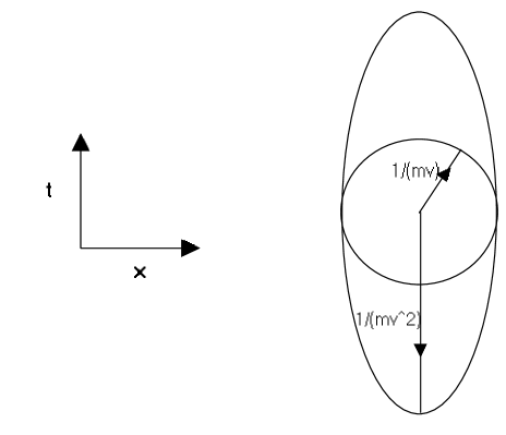
Figure 13: The soft gluons and heavy quarks have differing spatio-temporal extent, The overlap regions, which determines the scaling of the measure in the action is of order $(v,v)$

II.5 Calculating Loops in NRQCD

Now let us take stock in what we have built. So far we have a leading order action which contains the kinetic pieces for the fermions and gluons (75) and (87), as well as two leading order interactions (78) and (85). If we want to match beyond leading order in $\alpha$, we need to know how to calculate using our effective theory. Calculating loop graphs seems rather complicated given that we will have loops with sums over labels. However, it will turn out in the end to be quite simple. As a first example suppose we’re interested in a loop consisting of two insertions of $L_{C}$, as shown in figure (14).

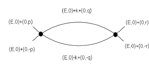
Figure 14: A one loop graph in the effective theory with two insertions of the coulomb interaction (solid dot).

The external fermions have energy $E$ and momenta $\pm{\bf\vec{p}},{\bf\vec{r}}$. In the effective theory, the external fermions have soft momentum (labels) $\pm{\bf\vec{p}},\pm{\bf\vec{r}}$, and the ultra-soft momentum $(E,0)$. The intermediate fermions in the effective theory have soft momentum $\pm q$, and ultra-soft momentum $(E,0)\pm k$. The graph in the effective theory is proportional to the integral

$$I_{Coul}=\sum_{\bf\vec{q}}\int d^{4}k{1\over{\bf(\vec{p}-\vec{q})^{2}}}\ {1\over{\bf(\vec{r}-\vec{q})^{2}}}\ {1\over k^{0}+E-{\bf\vec{q}}^{2}/2m+i\epsilon}\ {1\over-k^{0}+E-{\bf q}^{2}/2m+i\epsilon}.$$ (88)

There is an integral over the ultra-soft energy $k^{0}$, the ultra-soft momentum $\mathbf{k}$, and a sum over the soft momentum $\mathbf{q}$. Summing over ${\bf\vec{q}}$ and integrating over ${\bf\vec{k}}$ is equivalent to integrating over the entire momentum space. Thus one can replace Eq. (88) by

$$I_{Coul}=\int d^{4}q{1\over({\bf\vec{p}}-{\bf\vec{q}})^{2}}~{}{1\over({\bf\vec{r}}-{\bf\vec{q}})^{2}}~{}{1\over q^{0}+E-{{\bf\vec{q}}}^{2}/2m+i\epsilon}~{}{1\over-q^{0}+E-{{\bf\vec{q}}}^{2}/2m+i\epsilon},$$ (89)

where

$$dk^{0}\to dq^{0},\qquad\sum_{\mathbf{q}}\int d{\mathbf{k}}\to\int d{\mathbf{q}}.$$ (90)

Soft loops are treated in a similar fashion. Consider the diagram with the insertion of two soft interactions as shown in figure (15).

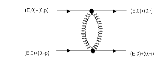
Figure 15: A one loop graph in the effective theory with two insertions of the soft interaction (solid dot).

It gives a contribution of the form

$$I_{soft}=\sum_{q}\int d^{4}k{1\over{\bf(\vec{p}-\vec{r})^{2}}}\ {1\over{\bf(\vec{p}-\vec{r})^{2}}}\ {1\over\left(q^{0}\right)^{2}-{\bf\vec{q}}^{2}}\ {1\over\left(q^{0}\right)^{2}-\left({\bf\vec{q}+\vec{p}-\vec{r}}\right)^{2}},$$ (91)

where I have used the last interaction in Eq. (85) for the soft vertices. The sum on $q$ is over a four-vector. As in the case of the potential loops, we make the replacement

$$\sum_{q}\int d^{4}{k}\to\int d^{4}{q},$$ (92)

where the replacement must be done for all four components of $q$, since soft gluons carry a four-vector label $q$. There is a much simpler way to arrive at the effective theory integrand. Just take the full theory graphs, assume the proper scaling for the gluon loop momentum, i.e. soft, potential or US, and just keep the leading order term in each propagator.

II.6 Matching at Subleading Orders in $v$

Let us now consider to matching at higher orders in $v$, but still at tree level. We can guess the first correction to the kinetic energy from the dispersion relation

$$L^{(2)}_{kin}=\sum_{\bf{\vec{p}}}\psi^{\dagger}_{\bf{\vec{p}}}(\frac{\bf{\vec{p}}^{4}}{8m^{3}})\psi_{\bf{\vec{p}}}~{}+~{}(\psi\rightarrow\chi).$$ (93)

Formally this piece can be derived simply by keeping the sub-leading terms in the expansion of the QCD action in terms of the non-relativistic fields (74). The more relevant correction comes from higher order terms in the multipole expansion,

$$L^{(1)}_{mp}=\sum_{\bf{\vec{p}}}\psi^{\dagger}_{\bf{\vec{p}}}(\frac{\bf{\vec{p}}\cdot{i\bf\vec{D}}}{m})\psi_{\bf{\vec{p}}}~{}+~{}(\psi\rightarrow\chi).$$ (94)

The ultra-soft gluon field inside ${\bf\vec{D}}$ scales as $v^{2}$, as does the derivative since it brings down a factor of the residual momentum of the heavy quark. Now let’s consider the corrections to the quark/anti-quark potential. These are derived by expanding the full theory graph in figure (9) to higher orders in $v$.

Exercise 2.2 Show that, at order $\alpha_{s}v$ the subleading potentials generated by T-channel gluon exchange are given by

$$V^{(1)} = (T^{A}\otimes\overline{T}^{A})\left[{{V}_{r}\>{\bf\vec{p}^{2}}\over m^{2}\,{\bf\vec{k}}^{2}}+{V_{hf}\over m^{2}}\,{\bf\vec{S}}^{2}+{{V}_{so}\over m^{2}}\,\Lambda({\bf\vec{p}^{\prime},\vec{p}})+{V_{t}\over m^{2}}\,{T}({\bf\vec{k}})\right]$$ (95)

where ${\bf\vec{k}=\vec{p}-\vec{p}^{\prime}}$ and

$$\bf\vec{S} = {{\bf\vec{\sigma}_{1}+\vec{\sigma}_{2}}\over 2},\qquad\Lambda({\bf\vec{p}^{\prime},\vec{p}})=-i{\bf\vec{S}\cdot(\vec{p}^{\prime}\times\vec{p})\over{\bf k}^{2}},\qquad{T}({\bf\vec{k}})={\bf\vec{\sigma}_{1}\cdot\vec{\sigma}_{2}}-{3\,{\bf\vec{k}\cdot\vec{\sigma}_{1}}\,{\bf\vec{k}\cdot\vec{\sigma}_{2}}\over{\bf k}^{2}}$$

and ${\bf\vec{\sigma}}_{1}/2$ and ${\bf\vec{\sigma}}_{2}/2$ are the spin-operators on the quark and anti-quark. $V_{hf}$ and $V_{so}$ are the familiar hyperfine and spin-orbit potentials respectively. The matching coefficients are given by

$${V}_{r} = 4\pi\alpha_{s}\,,\qquad{V}_{hf}=-\frac{4\pi\alpha_{s}}{3}\,,\qquad$$

$${V}_{so} = -6\pi\alpha_{s}\,,\qquad{V}_{t}=-\frac{\pi\alpha_{s}}{3}.$$ (96)

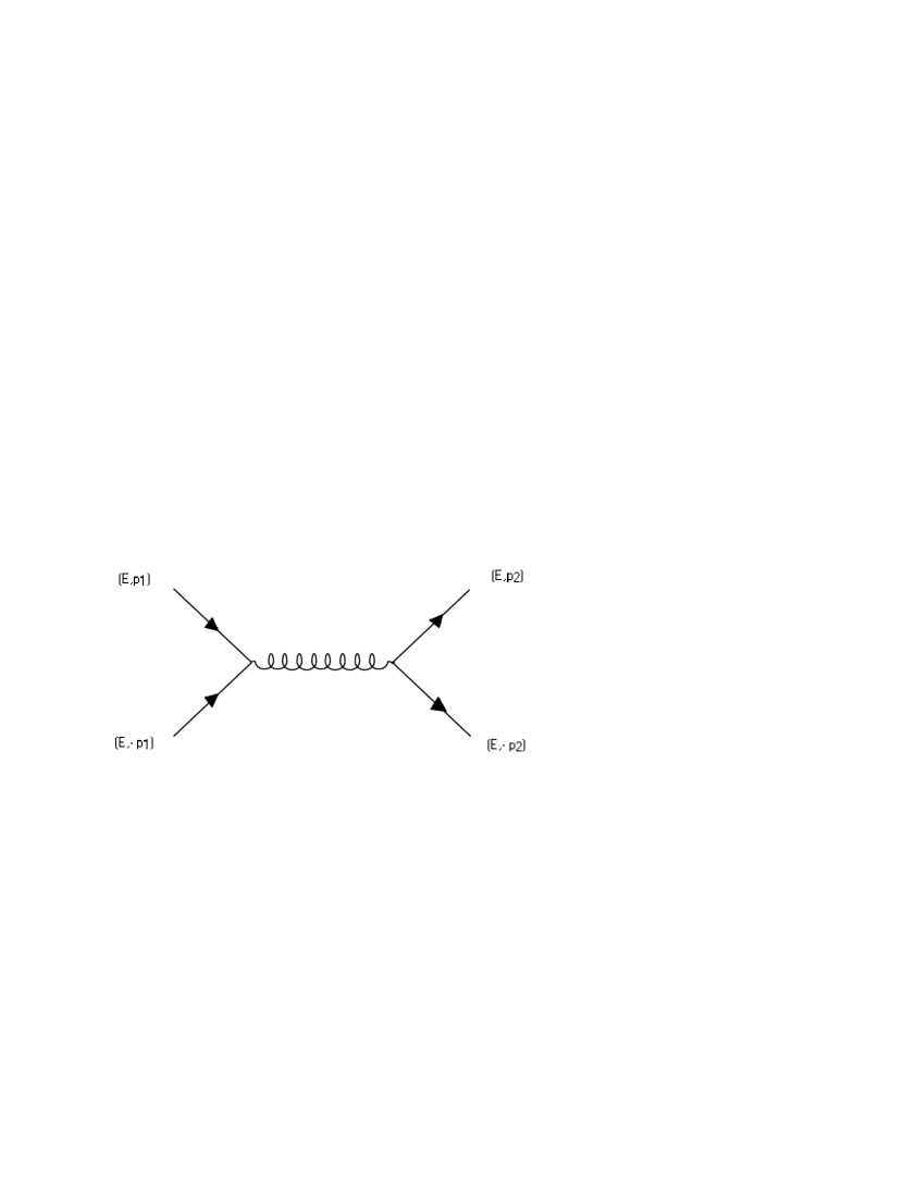
Figure 16: Tree level full theory diagram contributing to the potential.

The annihilation diagram in Fig. 16 generates terms of order $\alpha_{s}v$ in the potential. Using Fierz identities and charge conjugation, the contribution of this diagram can be transformed into the basis in Eq. (95) and give additional contributions to the matching. Only ${V}_{hf}$ receives a non-zero contributions at tree level from annihilation:

$$V_{hf,a}={1\over N_{c}}\>\pi\,\alpha_{s}\,,\qquad$$ (97)

where the subscript $a$ stands for annihilation. In addition this diagram generates the a hyper-fine interaction with a different color structure

$$\delta V^{(1)}=(1\times 1){V_{hf}^{(1)}\over m^{2}}\>{\bf S}^{2}$$ (98)

with $V_{hf}^{(1)}=\alpha\pi{N_{c}^{2}-1\over{2N_{c}}}$. The color factor arises from the Fierz rearrangement.

II.7 Matching at Subleading Orders in $\alpha$

Let’s now consider matching beyond tree level. But before we plunge into a calculation we must address an intricacy of NRQCD which I touched upon previously. In particular, we noticed that the Coulomb potential scales as $1/v$. On the face of it, this presents a serious problem to the theory for the following reason. Suppose we wish to calculate the matrix element of some operator in the effective theory, $\langle\psi\mid O\mid\psi\rangle$. at order in $v^{k}$. In this case we have

$$\langle\psi\mid O\mid\psi\rangle=\int d^{4}x_{1}...d^{4}x_{n}\langle\psi\mid T(OH_{1}(x_{2})....H_{n}(x_{n})exp({i\int d^{4}xL_{C}(x)})\mid\psi\rangle$$ (99)

where $H_{i}$ are terms in the sub-leading Hamiltonian such that their net order in $v$ is $v^{k}$. Given that the contribution from the Coulomb potential is of order $1/v$ and must be treated non-perturbatively, it appears that the time ordered product will not have a definite scaling in $v$. However, we are saved by the fact that while the Coulomb potential is of order $1/v$ it is also of order $\alpha$. Furthermore, in a Coulombic state the Virial theorem tells us that

$${mv^{2}}\simeq{\alpha_{s}(1/r\simeq mv)\over{r}}$$ (100)

so that $\alpha_{s}(mv)\simeq v$.

So when we calculate matrix elements we should treat the Coulomb potential to be order one. However, when we match, we must account for the fact that the Coulomb potential can enhance a sub-leading operator, at the cost of a power of $\alpha_{s}$. For instance, if we want to match at order $\alpha_{s}^{2}$, then we have to include contributions of the form

$$\langle L^{(2)}L_{c}^{2}\rangle\propto\alpha_{s}^{2}$$ (101)

where $L^{(2)}$ is an order $v^{2}\alpha_{s}^{0}$ piece of the Lagrangian.

As a practical example let us consider the matching of a production current at order $v^{0}$. This matching calculation is relevant to top-quark threshold production HMST . At tree level we match by expanding the full QCD current in terms of the NRQCD fields,

$$\bar{q}\gamma^{i}q=\sum_{\bf\vec{p}}\psi^{\dagger}_{\bf\vec{p}}\sigma^{i}\chi^{\star}_{\bf-\vec{p}}+...$$ (102)

This operator produces a quark/anti-quark pair in a relative ${}^{3}S_{1}$ state.

Exercise 2.3 Show that at order $v^{2}$ one generates the operators

$$O_{1}^{i}=\sum_{\bf\vec{p}}\psi^{\dagger}_{\bf\vec{p}}({\bf\vec{p}\cdot\vec{\sigma}}){\bf p^{i}}\chi^{\star}_{\bf-\vec{p}}$$ (103)

$$O_{2}^{i}=\sum_{\bf\vec{p}}\psi^{\dagger}_{\bf\vec{p}}({\bf\vec{p}^{2}})\sigma^{i}\chi^{\star}_{\bf-\vec{p}}$$ (104)

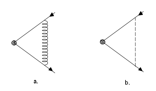
Figure 17: One loop matching diagrams in the full and effective theory. In the effective theory there are additional diagrams involving temporal US gluons which vanish.

At one loop we must calculate the graphs shown in (17). Since the full theory current is conserved, it has vanishing anomalous dimension once the wave function renormalization is included. We can simplify the matching calculation by working at threshold. In this way the effective theory diagram vanishes, since it is scaleless. Calculating the full theory diagram gives

$$\rm{Figa}=\psi^{\dagger}\sigma^{i}\chi^{\star}\frac{i\alpha C_{F}}{4\pi}\left[\frac{1}{\bar{\epsilon}_{UV}}+\frac{2}{\bar{\epsilon}_{IR}}-3\ln(m^{2}/\mu^{2})-9\right],$$ (105)

where I have explicitly separated the UV from the IR divergences. Adding the contribution from the wave function renormalization, all the UV and IR poles cancel. We then find the matching coefficient to be

$$C=(1-2C_{F}\frac{\alpha}{\pi}).$$ (106)

You should be able to show for yourself that this short cut to calculating the matching coefficient is identical to calculating the hard piece of the graph using the method of regions.

Notice that at one loop the current has no anomalous dimension. We can conclude this from the fact that all of the IR poles in the full theory cancelled (see section 1.8.2) In general we would not expect this since in the effective theory the current does not generate a symmetry. In fact we will see that at two loops we will generate an anomalous dimension.

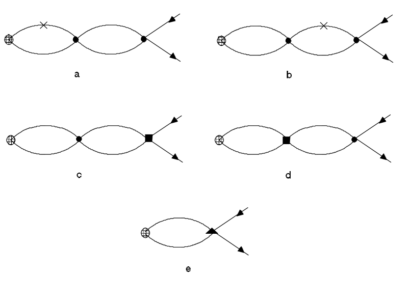
Figure 18: Diagrams contributing to the matching of the current at order $\alpha^{2}v^{0}$. The large hatched circle is the current insertion. The small filled circle is a Coulomb potential while the square represents insertions of order $v^{1}$ potential. The cross corresponds to the insertion of the $p^{4}/(8m^{3})$ operator. The triangle is the order $v^{0}$ potential.

At two loops one must account for the possible Coulomb enhancement discussed previously in this section. So if we concerned with contributions of order $\alpha_{s}^{2}v^{0}$, we must include all possible operator insertion such that the net power is $v^{0}$. This means we must also include any order $v^{0}\alpha_{s}^{2}$ potentials which might be generated. At this order the full theory generates the $v^{0}$ potential

$$V^{(0)}=V_{k}\frac{\pi^{2}}{m\mid{\bf\vec{k}}\mid}\\$$

where

$$V_{k}=\alpha^{2}(\frac{C_{F}^{2}}{2}-C_{A}C_{F}),$$ (107)

and I have projected the potential onto the color singlet channel since that is all we need when calculating the production current. We must include one insertion of this potential in addition to insertions of the order $v$ potentials already discussed in the previous section. The relevant diagrams are shown in (18).

In addition there are corrections which contain Coulomb singularities $1/v$, i.e. those contributions whose net scaling has inverse powers of $v$. However, these won’t contribute to the matching since they will cancel in the full and effective theory. The purpose of this example was just to illustrate that when you match you must remember that sub-leading operators can be enhanced due to the $1/v$ nature of the Coulomb potential. To my knowledge, as of the time of this writing, this subtlety is unique to NRQCD. It is interesting to note that had we done the two loop calculation using HQET propagators we would get a vanishing anomalous dimension. This is most easily seen in $A_{0}=0$ gauge.

Exercise 2.4: Prove that in the ${\overline{MS}}$ scheme the anomalous dimensions of the production current is gauge invariant. To prove this write down two equations for the current. One imposing its independence from $\mu$ and the other its independence of the gauge fixing parameter $\alpha$. Then commute the two equations to derive a set of relations which allows you to complete the proof. If you get stuck consult the original reference CW .

The reason HQET gets it wrong lies in the theory’s inability to properly describe fermion-fermion propagation. What happens is that HQET misses out on the Coulomb singularity. This fact emphasizes an important point about NRQCD. You can’t treat the scales $mv$ and $mv^{2}$ independently. Usually we would argue that between the scales $m$ and $mv$, $mv^{2}$ should be treatable as a perturbation, much as we would treat a light quark mass when working at a scale $E\gg m_{q}$. But the fact that we need to keep the kinetic piece of the action at leading order is telling us that both $mv$ and $mv^{2}$ must exist simultaneously in the theory. After a brief diversion we will see the consequences of this correlation of scales.

II.8 Summing Logs: The Velocity Renormalization Group (VRG)

You have probably noticed that I have been careful not to specify the scale at which to evaluate the running couplings $\alpha_{s}(\mu)$. Such a specification implies we have control of the logarithmic corrections, which I will only now discuss. As shown in the previous lecture the recipe for summing large logs is typically straightforward. Suppose we have a theory with two “large” (relative to the scale at which experiments are to be performed $E$) scales $m_{1}\gg m_{2}$. In a general diagram we would expect to generate logs of the form $\ln(m_{2}/E),~{}\ln(m_{1}/E),~{}\ln(m_{1}/m_{2})$. We would sum these large logs in steps: 1) Match at the scale $m_{1}$ onto a theory where $\phi_{1}$ has been integrated out. 2) Use the RG to run down to the scale $m_{2}$. 3) Match onto a theory where $\phi_{2}$ has been integrated out. 4) Run down to the scale of the experiment. We will call this procedure “two stage running”. In the case of NRQCD, where we have two large scales $m$ and $mv$ and a low energy scale of $mv^{2}$, we will get logs of the form $\ln(m/mv^{2})$ and $\ln(m/mv)$. So we might be tempted to follow the standard machinery and turn the crank. Match at $m$, run to $mv$ integrated modes of momenta $mv$ and then run down to the scale $mv^{2}$. However, NRQCD is a lot more interesting than that. The basic point is that the two scales $mv$ and $mv^{2}$ are correlated. They shouldn’t be treated independently, since they coexist in the fermionic propagator. If we were to follow the two stage running in NRQCD, we would first match at $m$ onto an HQET like theory by rescaling the fields only by their masses. In this case we should allow for quark virtualities $q^{2}<m_{Q}^{2}$ and one might wish to treat ${{\bf\vec{p}^{2}}\over{2m}}$ as a perturbation leaving the HQET form of the propagators. But as we discussed above, we know that this will give the wrong anomalous dimension for the current lmr . Instead, in NRQCD what we must do is match directly, at the scale $m$, onto the theory in which $E\approx{{\bf\vec{p}^{2}}\over{2m}}$. So we can see immediately that the two stage running will not be appropriate. Instead we do what is known as “one stage running”.

Given that we have to match directly onto a theory in which two scales exist simultaneously, how can we sum the large logs? In general, potential and soft loops will generate $\ln(\sqrt{mE}/\mu)$, while US loops will introduce logs of the form $\ln(E/\mu)$. So in one-stage running we introduce two different $\mu$ parameters, $\mu_{S}$ and $\mu_{US}$. However, we are not free to choose $\mu_{S}$ and $\mu_{US}$ independently, since $\mu_{S}^{2}=m\mu_{US}$. Instead we should write $\mu_{S}=m\nu$ and $\mu_{US}=m\nu^{2}$, and think of a subtraction velocity $\nu$ instead of a subtraction scale $\mu$. This is the basis of what is known as the “velocity renormalization group” (VRG)lmr . The renormalization group equation is then derived using the fact that bare quantities are independent of the subtraction velocity, i.e.

$$\nu\frac{d}{d\nu}G_{B}=0.$$ (108)

Then by solving these equations and running from $\nu=1$ to $\nu=v$, we can sum all the large logs. How does the VRG differ from the standard RG MSS ? In VRG we have

$$\nu\frac{d}{d\nu}=\nu(\frac{d\mu_{S}}{d\nu}\frac{d}{d\mu_{S}}+\frac{d\mu_{US}}{d\nu}\frac{d}{d\mu_{US}})=\mu_{S}\frac{d}{d\mu_{S}}+2\mu_{US}\frac{d}{d\mu_{US}}.$$ (109)

Note, the crucial factor of $2.$ In the two-stage method one would first integrate from $m$ to $mv$ using, $\gamma_{S}+\gamma_{US}$, then continue down to the scale $mv^{2}$, using only $\gamma_{US}$. Whereas in one-stage one integrates $\gamma_{S}+2\gamma_{US}$ from $\nu=1$ to $\nu=v$. If we assume that the anomalous dimensions are constant and don’t run, then in the two stage running we would find for the running of some generic Wilson coefficient

$$C(mv^{2})-C(m)=(\gamma_{S}+\gamma_{US})\ln(mv/m)+\gamma_{US}\ln(mv^{2}/(mv)),$$ (110)

while in one-stage we have

$$C(mv^{2})-C(m)=(\gamma_{S}+2\gamma_{US})\ln(v).$$ (111)

So we have agreement. However, in general the anomalous dimensions depend upon some couplings which are scale dependent. This scale dependence will lead to a discrepancy between the two methods at higher orders.

Suppose we are interested in the anomalous dimensions $\gamma_{i}$ of some set of Wilson coefficients $U_{i}$ . These anomalous dimensions will, in general, depend on $U_{i}$ themselves.

$$\gamma_{i}\equiv\gamma_{i}(U_{i}(\mu)).$$ (112)

$\gamma_{i}$ will be some function of $t\equiv\ln(\mu)=\ln(v)$, which we can expand

$$\gamma_{i}(t) = \gamma_{i}(0)+t\left(\frac{\partial\gamma_{i}}{\partial U_{k}}\frac{\partial U_{k}}{\partial t}\right)_{t=0}+...$$ (113)

$$= \gamma_{i}(0)+t\left(\frac{\partial\gamma_{i}}{\partial U_{k}}\gamma_{k}\right)_{t=0}+...~{}~{}~{}~{}.$$

Suppose the $U_{i}$ have both soft and ultra-soft anomalous dimension (this typically will occur at two loops). Then in one-stage running, integrating the anomalous dimensions will give

$$\int_{0}^{t}\gamma_{i}(t^{\prime})dt^{\prime}=$$

$$t(\gamma_{i}^{S}+2\gamma_{i}^{US})+\frac{t^{2}}{2}\left(\frac{\partial\gamma_{i}^{S}}{\partial U_{k}}\gamma_{k}^{S}+\frac{\partial\gamma_{i}^{S}}{\partial U_{k}}(2\gamma_{k}^{US})+\frac{\partial(2\gamma_{i}^{US})}{\partial U_{k}}\gamma_{k}^{S}+\frac{\partial(2\gamma_{i}^{US})}{\partial U_{k}}(2\gamma_{k}^{US})\right).$$

Whereas two-stage running yields

$$\int_{0}^{\ln(v)}\gamma_{i}^{(S,US)}(t^{\prime})dt^{\prime}+\int_{\ln(v)}^{\ln(v^{2})}\gamma_{i}^{(S)}(t^{\prime})dt^{\prime}=$$

$$t(\gamma_{i}^{S}+2\gamma_{i}^{US})+\frac{t^{2}}{2}\left(\frac{\partial\gamma_{i}^{S}}{\partial U_{k}}\gamma_{k}^{S}+\frac{\partial\gamma_{i}^{S}}{\partial U_{k}}(\gamma_{k}^{US})+\frac{\partial(\gamma_{i}^{US})}{\partial U_{k}}\gamma_{k}^{S}+4\frac{\partial(\gamma_{i}^{US})}{\partial U_{k}}(\gamma_{k}^{US})\right),$$

and we see that the cross terms differ by a factor of two.

Let us now return to the question of the running of the Coulomb potential. This running is particularly simple because the renormalization only involves soft loops. The matching coefficient is simply $4\pi\alpha_{s}(m)$, and the running is generated by figure (15), with each vertex giving a factor of $V_{c}$

$$Fig.15=-i\frac{\alpha_{s}^{2}}{{\bf\vec{k}}^{2}}(T^{A}\otimes\bar{T}^{A})\left(\frac{11}{3}C_{A}\left(\frac{1}{\bar{\epsilon}}+\ln\left(\frac{\mu_{S}^{2}}{{\bf\vec{k}}^{2}}\right)\right)+\frac{31C_{A}}{9}\right).$$ (116)

There are also corrections stemming from US temporal gluon loops, but these vanish for reasons which were previously discussed. Calling the coefficient of the Coulomb operator in the action $V_{c}$, and using the fact that its bare value $(V_{c}^{B}$) is independent of $\nu$, we have

$$\nu\frac{d}{d\nu}V_{c}^{B}=0=\nu\frac{d}{d\nu}\left(\mu_{S}^{-2\epsilon}(V_{c}-\frac{11}{3}C_{A}\frac{\alpha_{s}^{2}}{\epsilon})\right),$$ (117)

and we are left with

$$\nu\frac{d}{d\nu}V_{c}=-2\beta_{0}\alpha_{s}^{2}(\nu).$$ (118)

Where I’ve used $\beta_{0}=\frac{11}{3}C_{A}$ to make it clear that $V_{c}$ obeys the same equation as the gauge coupling. Using our matching result for an initial condition, along with the explicit form for $\alpha_{s}(\nu)$, we find

$$V_{c}(m\nu)=4\pi\alpha_{s}(m\nu).$$ (119)

At this order the running of the potential is identical to the running of the beta function. The large logs can be avoided by choosing $\alpha({\bf\mid\vec{k}\mid})$ in the potential. This agrees with our intuitive picture of the force law (Wilson loop) getting quantum corrections due to the running of the coupling. However, this correspondence does not persist at higher orders as the running of the Coulomb potential includes effects from higher order potentials which vanish in the static limit BPSV ; HMS .

Exercise 2.5: Show that the $\frac{11}{3}C_{A}$ gets replaced by the the full beta function $\beta_{0}=\frac{11}{3}C_{A}-\frac{2}{3}n_{f}$, once $n_{f}$ soft light quark fields, $\phi_{q}$, are introduced. To begin this calculation first show that the soft Lagrangian gets an additional piece given by

$$L_{S}^{\prime}=-g^{2}\sum_{{\bf\vec{p},\vec{p}^{\prime}},q,q^{\prime}}\left(\frac{1}{(\bf{\vec{p}^{\prime}-\vec{p}})^{2}}(\psi^{\dagger}_{\bf\vec{p}^{\prime}}T^{A}\psi_{\bf\vec{p}})(\bar{\phi}_{q^{\prime}}\gamma_{0}T^{A}\phi_{q})\right)+(\psi\rightarrow\chi).$$ (120)

There is a simple way to determine when, where and how the $\mu_{S}$ and $\mu_{US}$ show up. We just make sure that in $4-2\epsilon$ dimensions, the operators have the same $v$ scalings as they would in $4$ dimensions. For instance, in the Coulomb potential the matching comes with a factor of $g^{2}$, which arises from an exchange of a Coulomb gluon. In $4-2\epsilon$ dimensions, should we write this as $g^{2}\mu_{S}^{2\epsilon}$ or $g^{2}\mu_{US}^{2\epsilon}$? The coupling should still have units $(mass)^{\epsilon}$ but the $v$ scaling appears ambiguous until we impose the fact that the operator should scale as $v^{-1}$. The fermion fields now scale as $v^{3/2-\epsilon}$ and we have a factor of $1/v^{2}$ from the Wilson (label) coefficient. But now the measure scales as $v^{-2}v^{-3+2\epsilon}$. So to insure that the operator scales as $v^{-1}$ we should write $g^{2}\rightarrow g^{2}\mu_{S}^{2\epsilon}$. If we consider an operator where a US gluon attaches to the potential MSI , the scaling of the measure won’t change (see section 2.4) but since the US gluon scales as $v^{2-2\epsilon}$ then we should include a factor of $\mu_{US}^{\epsilon}\mu_{S}^{2\epsilon}$.

II.9 The Lamb Shift in QED

I would now like to utilize this formalism in a simple setting, namely, the Lamb shift in QED. This is a beautiful example because, not only does the formalism simplify the calculation, but it also provides one with immediate information about sub-leading orders, as we shall see. Let me remind you that the Lamb shift is the splitting between the $2S_{J=1/2}$ and $2P_{J=1/2}$ levels of Hydrogen. Recall that these levels are “accidentally” degenerate up to $\alpha^{2}$ corrections. Their splitting comes in at relative order $\alpha^{3}$, corresponding to a over all energy shift of order $\alpha^{5}$. This splitting is dominated by the so-called “Bethe log”, $\alpha^{5}\ln v$. From an effective field theory point of view, all logs are RG logs. If they look like “long distance” logs, its only because the scales have not been properly separated, i.e. you haven’t written down the proper effective field theory. Thus, we should be able to also resum these logs if there are more of them. In the case of the “Bethe log” one can ask the question, is this log just a first term in a series? i.e.

$$\Delta E\approx\alpha^{5}\ln v(1+\alpha\ln v+\alpha^{2}\ln^{2}v+...)$$ (121)

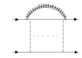
Figure 19: The QED diagram responsible for the Lamb shift. The photon over the top is non-instantaneous, i.e. ultra-soft, while the ladder gluons are Coulombic and must be resummed.

Typically the Lamb shift comes about from a low energy matrix element involving diagrams as shown in (19). But in NRQCD we know that there should be no large logs in any low energy matrix element. The log should arise from running. Let’s see how this comes about.

Recall that the leading order energy levels scale as $v^{2}$, or using the Coulombic counting, $\alpha\propto v$, $\alpha^{2}$. So one would expect at order $v^{4}$ there would be a splitting due to the subleading contribution to the Hamiltonian (II.9) and (II.7). However, we must account for the fact that in Hydrogen the masses of the constituents are not equal. In fact, we may take the mass of the proton to infinity.

Exercises 2.6: Show that for hydrogen we have

$$V^{(1)} = \left[{V_{so}\over m^{2}}\,\Lambda({\bf\vec{p}^{\prime},\vec{p}})+V_{2}\right]$$

where $V_{2}$ is a contact delta function potential which vanishes in the equal mass case (considered in (95)). Matching at $\nu=1$ we find

$$V_{2}(\nu=1)=\frac{\pi\alpha}{2}\left(\frac{1}{m_{e}}-\frac{1}{m_{P}}\right)^{2}\approx\frac{\pi\alpha}{2m_{e}^{2}}.$$ (123)

In addition, at this order, we should include corrections from the operator

$$L^{(2)}_{kin}=\sum_{\bf{\vec{p}}}\psi^{\dagger}_{\bf{\vec{p}}}(\frac{\bf{\vec{p}}^{4}}{8m^{3}})\psi_{\bf{\vec{p}}}~{}+~{}(\psi\rightarrow\chi).$$ (124)

Thus the mass splitting is given by

$$\Delta E=\langle^{2}\!S_{1/2}\!\mid L^{(2)}_{kin}+V_{2}\mid\!^{2}\!S_{1/2}\rangle-\langle^{2}\!P_{1/2}\mid L^{(2)}_{kin}+{V_{so}\over m^{2}}\,\Lambda({\bf\vec{p}^{\prime},\vec{p}})\mid\!^{2}\!P_{1/2}\rangle.$$ (125)

Calculating these matrix elements is nothing more than solving the Coulomb problem to first order in perturbation theory, which we can solve quantum mechanicallyTY . That is why it is simple to see that $V_{2}$ does not contribute to the energy shift in the $P$ wave since its wave function vanishes at the origin. The degeneracy is only split once we consider the running of $V_{2}$ and $V_{\Lambda}$. $L^{(2)}_{kin}$ is not renormalized due to reparameterization invariance but $V_{2}$ gets an anomalous dimensions from the diagram shown in (20).

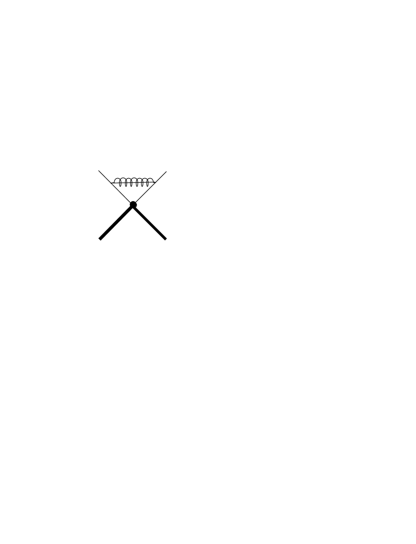
Figure 20: The one loop diagram which generates an anomalous dimension for $V_{2}$. The heavy lines are protons while the photon line with a line through it is ultra-soft. In the limit where the proton mass goes to infinity there is no soft anomalous dimension for $V_{2}$. The filled circle is a Coulomb vertex, while the US gluon couples to the electron via the order $v$ dipole operator (94).

A short calculation yields the result

$$\gamma_{2}=\frac{2\alpha}{3\pi m_{e}^{2}}$$ (126)

where $V_{c}=-4\pi\alpha$. Because we are looking at a one loop diagram involving only $US$ loops the VRG reduces to the usual RG (except of course for the factor of two arising from the fact that $\mu_{US}=m\nu^{2}$) and we have

$$\nu\frac{d}{d\nu}V_{2}=\gamma_{2}$$ (127)

since in QED the coupling doesn’t run below the scale $m_{e}$, the solution to the RG equation is trivial

$$V_{2}(\nu=v)=\gamma_{2}V_{c}\ln(v)+V_{2}(1).$$ (128)

We thus see that the series does indeed terminate. QED has a hard time generating logs because the coupling freezes below the scale $m_{e}$. At leading order the spin orbit potential has a vanishing anomalous dimension, so the energy splitting can be determined by taking the matrix element (125), but this time renormalized at the scale $\nu=v$, using

$$\langle V_{2}\rangle=\gamma_{2}V_{c}\ln(\nu)\mid\!\psi(0)\!\mid^{2}.$$ (129)

and

$$\mid\!\psi(0)\!\mid^{2}=\frac{(m\alpha)^{3}}{\pi n^{3}}$$ (130)

we find the famous result

$$\Delta E=-\frac{m\alpha^{5}}{3\pi}\ln(v),$$ (131)

and we see that the series does indeed terminate at order $\alpha^{5}\ln(v)$. Using effective field theory we can go a step further and ask questions about the next series of logs,

$$\alpha^{5}(\alpha\ln(v)+\alpha^{2}\ln^{2}(v)+...)$$ (132)

It turns out MSQED , that this series terminates as well at order $\alpha^{8}\ln^{3}(v)$. The reason the series terminates, is due the fact that the coupling in QED does not run below the scale of the electron mass. In QCD the series is not so simple.

II.10 States in the Effective Theory

Before closing out this lecture I would like to emphasize an important point about the states in any effective theory. If we wish to keep our ducks in a row we should be sure to treat the states of the effective theory as eigenstates of the lowest order piece of the action. Power corrections to the states come from taking time ordered products in the low energy matrix elements. This is exactly what we do in quantum mechanics. We perturb around the lowest order wave functions. In this way we can keep track of various power law corrections. It is a simple exercise to see exactly how this works generically. Suppose we are considering a correction to the expectation value for some transition operator

$$\mbox{{T}}=\int d^{4}y\langle\Phi_{1}(p_{1})\mid T(O(0)H_{1}(y))\mid\Phi_{2}(p_{2})\rangle$$ (133)

where $\Phi_{i}$ are eigenstates of $H_{0}$. The two time orderings correspond to corrections to $\Phi_{1}$ and $\Phi_{2}$. Let’s consider the contribution from $y_{0}<0$. Using the representation of the theta function

$$\theta(-y_{0})=\frac{1}{i\pi}\int^{\infty}_{-\infty}d\tau\frac{e^{-iy_{0}\tau}}{\tau+i\epsilon}$$ (134)

and inserting a complete set of states yields

T $$= \sum_{n}\int d^{4}y\frac{1}{i\pi}\int^{\infty}_{\infty}d\tau e^{iy_{0}(p_{2}-p_{n}-\tau)}\langle\Phi_{1}(p_{1})\mid O(0)\mid n^{(0)}\rangle\frac{\langle n^{(0)}\mid H_{1}(0)\mid\Phi_{2}(p_{2})\rangle}{E_{2}-E_{n}}.$$

Then recalling from basic time independent perturbation theory that the first correction ($\psi^{(1)}$) to the zeroth order eigenstate ($\psi^{0}$) of the full Hamiltonian $H=H_{0}+H_{1}$ is given by

$$\mid\psi^{(1)}\rangle=\sum_{n\neq 0}\mid n^{(0)}\rangle\frac{\langle n^{(0)}\mid H_{1}\mid\psi^{(0)}\rangle}{E_{0}-E_{n}}$$ (136)

we explicitly see that the time ordered product accounts for corrections to the wave function.

Let me emphasize that there is nothing wrong with treating the physical states as eigenstates of the exact Hamiltonian. This is often done in the literature. One often reads about “higher Fock states” of a bound state. For instance in the case of NRQCD one often hears the term “dynamical gluons” as being part of a higher Fock state of the onium. Again, there is nothing wrong with this, it just goes against the spirit of effective field theory as espoused in these lectures. But there are advantages to treating the states as lowest order eigenstates. For instance, in the case of HQET the leading power corrections to the meson masses coming from the operators

$$O_{1}=\bar{h}_{v}\frac{\vec{D}^{2}}{2m_{Q}}h_{v}~{}~{}~{}~{}O_{2}=\bar{h}_{v}\frac{g\sigma_{\mu\nu}G^{\mu\nu}}{4m_{Q}}h_{v}$$ (137)

are cleanly separated from higher order power corrections. This would not be true if we took the meson to be an eigenstate of the full Hamiltonian since the expectation values of $O_{1}$ and $O_{2}$ would contain contributions of order $1/m^{2}$. Of course this would only be an issue if we were interested in $1/m^{2}$ corrections.

II.11 Summary

In this second lecture I have introduced some new concepts into the game. In particular, the idea that one can integrate out massless particles by breaking up the field into various components. In the case of NRQCD we split up the gluon field into four types of modes: hard $(m,m)$, though I didn’t use this term previously. These are just the gluons which we integrate out when we match at the scale $m$. Potential $(mv^{2},mv)$, soft $(mv,mv)$ and ultra-soft $(mv^{2},mv^{2})$. These last 3 modes are believed to be sufficient to correctly reproduce all the non-analytic structure of non-relativistic Greens function. To date this has only been proven up to two loops. Once we determined the modes, we fixed their couplings by matching, although gauge invariance and RPI fix many such couplings without doing any work. The way we arrived at the proper mode decomposition was far from systematic. Indeed, finding the proper modes is more of an art form at this point. The potential and US modes fell out directly from matching, while we deduced the need for the soft modes from physical argument. Of course had we carried out the matching in the two quark sector we would have immediately seen the need for a soft mode. In particular, if you calculate the full QCD box diagram you will see that just including the potential and the US modes is not sufficient to reproduce the full result MoR .

There is no general rule for determining what modes are necessary. However, there are some guiding principles. First we must determine the scales involved in the external states of the theory. In the case of NRQCD, those would be $mv$ and $mv^{2}$. Then there are some obvious modes that one can pick out that are necessary. Those are modes which leave the external lines on shell. So for a fermion with momentum $(mv,mv^{2})$ we know that US and potential gluons should contribute to the non-analytic behavior of the Greens functions. After that, finding more modes starts to get harder and you have to do some matching calculations to be sure. But its pretty clear that the other modes should also be formed from these scales. So the soft $(mv,mv)$ modes are an obvious choice. Since these modes throw quarks off-shell, its clear that you will need more than one interaction vertex to generate an operator in the effective theory. Then what about $(mv,mv^{2})$ modes? Physically, these modes would mediate interactions which are non-local in time but local in space, which is clearly unphysical, and in fact a simple calculation shows that such modes can’t contribute. What about modes with higher powers of $v$ such as $mv^{3}$? It is simple to see that these modes would give zero since this scale can be dropped in all propagator, and so loop integrals would be independent of the loop variable itself. The interested reader should study SCETSCETI ; SCETII where similar mode deconstructions are performed.

III Lecture III: Effective Theories and Extra Dimensions

I would now like to discuss the application of effective field theories to the speculative topic of extra dimensions. The basic idea of using extra dimensions to unify forces goes back to the early part of the twentieth century with the work of Kaluza and Klein. But while extra dimensions have always played a role in string theory, from a phenomenological stand point the topic was dormant until a few years back. The reason for this dormancy was that the size of the extra dimensions was always assumed to be of order the Planck scale, and therefore, the measurable effects of the extra dimensions are so suppressed that they are irrelevant for all intents and purposes. However, with the advent of D-brane ideas, it was realized that the extra dimensions can be of arbitrarily large size (up to the experimental limits for gravity at short distanceswill ) since string theory provides a mechanism for field localization. That is, the usual problems involving observable effects of large extra-dimensions are eliminated because the standard model fields live on a fixed three dimensional space-like hyper-surface (the D-brane) and are thus impervious to the extra dimensions. This led to a flurry of model building, including new solutions to the hierarchy problem. Many of these models were discussed by other lecturers at this schoolDienes ; Csaki . My purpose here will be to treat these models from the point of view of effective field theories. Please note that I will be abusing the term $D-brane$ throughout the rest of these lectures. You many substitute the term $D-brane$ with a “domain wall of Planck scale thickness” for the purposes of these lectures.

Let us consider a generic theory on a manifold $M$ which can be written as a direct product

$${\it M}=M_{4}\times M_{d}$$ (138)

where $M_{d}$ is some $d$ dimensional compact manifold. We will assume for simplicity that there is only one relevant scale which characterizes $M_{d}$, namely $R$. So we would expect that for energies less than $1/R$, the effects of the compact extra dimensions should be suppressed by $ER\ll 1$. Let us study a $4+d$ dimensional gauge theory on this manifold where the coupling will have dimensions

$$[g]=-d/2.$$ (139)

Furthermore, naturalness tells us that $g\simeq R^{d/2}$. Since for $d>0$ the coupling is dimensionful, we would call this theory “non-renormalizable” in the old fashioned language. In our parlance we would simply say that its only an effective field theory, with limited predictive power. We would expect that this description of the theory would only correctly describe the physics up to a scale of order $\Lambda\equiv R^{-1}$. Typically the theory should contain a whole tower of higher dimensional operators which are suppressed by powers of $\Lambda$, which all become equally important when we have external momenta on this scale.

III.1 UV Fixed Points: A Theory Can Be More Than Effective

Now before going on I should say that the above conclusions need not necessarily hold. In particular, there could be a strongly coupled fixed point, where our power counting would break down. Indeed, as I previously mentioned, it is believed that there are five and six dimension supersymmetric Yang-Mills theories with 16 supercharges which posses non-trivial fixed points, although it is not known how to give Lagrangian descriptions of these theories. Our argument in the previous paragraph seems to exclude this possibility. So where is the loophole? The answer, is that our power counting arguments were all based upon reasoning which only necessarily holds at weak coupling. At strong coupling the power counting can change. While its not clear how this happens in the higher dimensional SUSY theories, there is a nice example in three dimensions BWP which illustrates a mechanism by which naive power counting breaks down.

Consider the theory of $N$ fermions in three dimensions interacting via a four Fermi interaction

$$L=\bar{\psi}_{i}i\partial\!\!\!\!/\psi_{i}+\frac{g^{2}}{2N}(\bar{\psi}_{i}\psi_{i})^{2},$$ (140)

In three dimensions the coupling $g^{2}/N$ has mass dimensions $-1$. So naively this theory is only an effective theory and breaks down at the scale $N/g^{2}$. However, it has been shown that in the large $N$ limit this is not the case. The conclusion that the theory is non-renormalizable was deduced from a weak coupling analysis. We know that quantum corrections can lead to scaling modifications. Typically, we study weakly coupled theory, where the quantum corrections only change the power counting by logs. But in strong coupling it can happen that this naive power counting breaks down, and a theory which we thought was non-renormalizable can indeed be renormalizable. This is exactly what happens if you study (140) in the large $N$ limit. The way this comes about is seen by re-writing (140) in terms of an auxiliary scalar field

$$L=\bar{\psi}_{i}i\partial\!\!\!\!/\psi_{i}+\sigma\bar{\psi}_{i}\psi_{i}-\frac{N}{2g^{2}}\sigma^{2}.$$ (141)

Now naively, the $\sigma$ propagator is constant. However, in the large $N$ limit we are forced to resum sets of diagrams, and in doing so the $\sigma$ propagator scales as $1/p$, if the bare coupling satisfies a certain bound. Given this scaling it is not hard, using textbook arguments, to show that all the divergences can be absorbed using only the operators shown in (141). This means that we can naturally set all the higher dimension operators in the action to zero without worrying that we will regenerate them via quantum corrections.

The point of this little diversion was just to let the reader know that sometimes field theories can actually be more than just effective, they may be complete. The trouble is that the strong coupling, which is necessary to generate large anomalous dimensions, makes it difficult to perform controlled approximations. So finding strongly coupled fixed points is a difficult task. I should also point out, that even without such a fixed point, there could well be a field theoretic description of the theory above the cut-off in terms of a different set of variables. For instance, the underlying theory could consist of a quiver gauge theory Cohen .

III.2 Naive Dimensional Analysis

Returning now to our non-renormalizable effective gauge theory, it actually turns out that there are simple arguments which lead to the conclusion that the scale at which the effective theory breaks down is numerically enhanced relative to the compactification scale by a geometrical factor. These arguments are based on what is called “naive dimensional analysis” which was first discussed in the context of chiral perturbation theory MG . A discussion of NDA within the context of super-symmetric theories can be found in NDASUSY . The basic argument goes as follows. Suppose we wish to calculate some n-point function ($G^{(n)}_{i}$) in a non-renormalizable field theory. Generically there will be a tree level contribution from some unknown counter-term ($C_{i}$), as well as some calculable (in terms of lower order coefficients) non-analytic terms which arise from loop corrections. Both contributions will be suppressed by powers of the UV scale $\Lambda$. Furthermore, dimensional analysis tells us that there is a correlation between the order in the loop expansion at which the observable is generated and the dimensionality of the operator which contributes to the observable at tree level.

Schematically the amplitude $M$ can be written as

$$M=(p^{2n}/\Lambda^{2n})\Big{(}C_{i}(\mu)+(C(\frac{1}{\epsilon}+\ln(p^{2}/\mu^{2}))+\kappa)\Big{)}$$ (142)

Here the piece proportional to $C_{i}$ is the contribution from some local operator, while the log piece comes from a loop integral involving lower order interactions whose couplings are related to $C$ by a geometric factor generated by the loop integration ($\rho$). That is, if $C_{0}$ is the lower order coupling then $C\simeq C_{0}^{2}\rho$. The divergence will get absorbed into $C_{i}$. The momentum $p$ represents some generic set of external momenta. Varying the renormalization scale on a interval of order one generates an effective change in result of order $C(p^{2n}/\Lambda^{2n})$. This is roughly equivalent to the statement that even if we set $C_{i}$ to zero at tree level, it will be generated at the loop level. Thus, we would expect that the size of the counter-term is thus naturally of order $Cp^{2n}/\Lambda^{2n}$. Now given that the log arises from a loop, $\rho$ is just a geometric factor which comes about from the angular integration and is of the form $1/(\gamma\pi^{r})$ where $\gamma$ and $r$ are a function of the number of dimensions. Thus NDA tells us that the cut-off is more like $\rho^{-1}\Lambda$ instead of $\Lambda$. While this does not seem like a huge distinction, the chiral Lagrangian description of low energy QCD would be far less powerful if it were no for this factor of $\rho=4\pi$. It is important to realize that NDA is a naturalness argument and assumes that couplings are all of order one. As such, it should only be taken as a guiding principle.

Let us now see how this works for a $4+d$ dimensional Yang-Mills theory. The leading interaction is suppressed by $\Lambda^{-d/2}$, so that any loop contribution to the effective action will be suppressed by $\Lambda^{d}$. Following the argument in the previous paragraph, let us compare the tree level contribution to the photon two point function arising from the higher dimensional operator

$$O_{2}=\frac{C_{2}}{\Lambda^{2}}F_{AB}\partial^{2}F^{AB}$$ (143)

to the contribution arising from loop corrections. The one loop correction to the two point function arising from interaction with a massless field is just the usual vacuum polarization graph, which in $4+d$ dimensions is given by

$$\pi(q^{2})\propto\frac{g^{2}}{(4\pi)^{2+d/2}}(-q^{2})^{d/2}\Gamma[-d/2].$$ (144)

where, as usual $\pi^{\mu\nu}(q^{2})=(q^{2}g^{\mu\nu}-q^{\mu}q^{\nu})\pi(q^{2})$. First we notice that the result only diverges in even dimensions. We could have guessed that since in odd dimensions there are no allowed (i.e. analytic) counter-terms which could absorb the divergence. So in odd dimensions we cannot use this particular calculation to learn anything from NDA. In even dimensions, e.g. $d=2$, we would conclude that the true cut-off is not $g^{-1}$ but $(g(4\pi)^{3/2})^{-1}$. Notice that I didn’t worry about the overall constants in (143). The full result could include group theory factors or gamma functions which might arise from doing Feynman parameter integrals. However, as I said before, NDA is only supposed to give you a rough guess of the true cut-off. I would not wager much on its exactness, but it does make qualitative sense that the cut-off will in general be enhanced by a geometric factor, which grows with the dimensionality.

Exercise 3.1 Using a physical argument determine whether one would expect the NDA guess for the strong coupling scale to change due to compactification.

III.3 The force law in $d$ dimensional Yang Mills Theory

It is interesting to try to understand the force law in a compactified version of a $d$ dimensional Yang-Mills theory. Let us calculate $V(r)$ a la exercise 1.6 for a five dimensional gauge theory compactified on an $S^{1}$ with radius $R$. If we KK reduce the theory (I am assuming here that the reader is familiar with KK reduction, otherwise see Csaki ), then the force will get contributions from zero mode as well as KK mode exchange between our heavy sources. For distances much larger than $R$ we would expect that only the zero mode force is non-negligible since the KK modes, whose masses scale with $n/R$, mediate a Yukawa force which dies off exponentially fast $e^{-rn/R}$. Thus, in this regime, we reproduce the four dimensional result, with a rescaled coupling $g/\sqrt{R}$. The rescaling arises from the the norm of the zero mode. On the other hand, for $r\ll R$, we can consider a whole tower of effectively massless $(R/n\ll r)$ KK modes each of which will contribute to the force. Thus, qualitatively we would expect the following behavior for the one loop force law at tree level

$$r\gg R : ~{}~{}~{}~{}~{}~{}~{}~{}V(r)\propto\frac{g^{2}}{Rr}$$

$$r\ll R : ~{}~{}~{}~{}~{}~{}~{}~{}V(r)\propto\frac{g^{2}}{r^{2}}$$ (145)

How will this result be modified by quantum corrections? At large $r\gg R$ we know that we should be dominated by external zero modes as well as zero modes in the loop. Whereas at small $r\ll R$ we will get contributions not only from corrections to zero mode exchange but also from corrections to the exchange of external KK modes as well.

At large $r$ the dominant correction will arise from the pure zero mode vacuum polarization diagram which generates a correction of the form

$$\delta V(r)\propto\frac{g^{4}}{rR^{2}}\ln(r),$$ (146)

whereas dimensional analysis tells us that the correction to the full five dimensional potential, at small $r$, will be of the form

$$\delta V(r)\propto\frac{g^{4}}{r^{3}},$$ (147)

so that at small $r$ the quantum corrections dominate the classical result as per our previous discussion.

Now let’s do an honest calculation to see what the exact result looks like. Instead of calculating the full five dimensional potential, I will concentrate on the potential generated by external zero modes and its correction. The reason being that this will be the relevant object to calculate when we discuss grand unification. I will do the calculation in two ways. First by working exactly in five dimensions, and then by matching and running, as discussed in the first lecture.

I will specialize to the case of scalar QED for simplicity. In this case there are two contributions to the vacuum polarization. The result for a massless scalar can be written as GnRII

$$\pi_{\mu\nu}(p^{2})=\frac{g^{2}}{R}\sum_{n}\int\frac{d^{d}k}{(2\pi)^{4}}\frac{1}{(k^{2}-m_{n}^{2})}\left[\frac{(2k+p)_{\mu}(2k+p)_{\nu}}{(p+k)^{2}-m_{n}^{2}}-2g_{\mu\nu}\right]\equiv(p_{\mu}p_{\nu}-p^{2}g_{\mu\nu})\pi(p^{2}).$$

$$\pi(p^{2})=\frac{g^{2}}{R}\left[\frac{\sqrt{p^{2}}R}{256}-\frac{1}{8\pi^{2}}\int_{0}^{1}xdx\sqrt{1-x^{2}}\ln(1-e^{-\pi xR\sqrt{p^{2}}})\right].$$ (149)

Exercise 3.2: Prove equation (149)

A few points are worth noticing here. First off the result is finite. This is because dimensional regularization sets the power divergence to zero. This finiteness may seem strange given that each mode gives a divergent contribution. What happens is that the sum of the poles cancels. Also, we would expect that at long distances we should exactly reproduce the four dimensional non-analytic behavior. So if we expand for small values of the momentum we should get a log and nothing else non-analytic. Defining $\delta=R\sqrt{p^{2}}$, and expanding the log we find

$$\ln(1-e^{\delta})=-\frac{\delta}{2}+\ln(\delta)+a_{1}\delta^{2}+a_{2}\delta^{4}+....$$ (150)

where the rest of the series contains only even powers of $\delta$. The first term in the expansion cancels the power dependence, the second term is the 4-D log and the higher order terms are analytic. At $pR\gg 1$, the result is dominated by the power dependence and taking the Fourier transform of the first term in the Dyson series we get back the radius independent result we would expect from dimensional analysis (147). We can also see from dimensional analysis that in the regime $pR\gg 1$ the theory becomes strongly coupled as all loops will be of the same order.

We should be able to reproduce the force law $p$ dependence by the running and matching procedure. For long distances $p<<R^{-1}$, all of the effects of the KK modes can be absorbed into local counter-terms and we simply reproduce the four dimensional result from the zero mode contribution. The higher KK modes just go into making up the low energy (measured) coupling. It is interesting though to see how we can reproduce the short distance behavior as well. If we are interested in the two point function at the scale $p$, then we should sum over all the KK modes with masses less than that scale. Each mode will contribute a $log(p/\mu)$ along with some scheme dependent constant. It seems clear how the linear dependence on $p$ will arise from summing over the constant pieces, but how does the $log(p)$ dependence becomes power-like?

Suppose we have measured the coupling at some scale below the first KK mass $M_{1}$. To predict the coupling at $P\simeq M_{1}$, we run the coupling to the scale $M_{1}$ using the four dimensional beta function, then we match, at the scale $M_{1}$, onto a theory which contains the zero mode as well as the first KK mode. In fact, let’s generalize this procedure. Suppose we know the value of the coupling at the scale $M_{n}$ and we wish to predict its value at some higher scale. We just match in steps as we discussed in the first lecture. Since we are only interested in the log piece let us ignore additive constants in the matching (even though in this particular case the constants are of the same order as the logs, so this calculation does not follow the standard systematics). Thus, at the order we are working we may use the relation

$$\alpha(\mu)=\frac{\alpha(\mu_{0})}{1-\beta_{0}n\alpha(\mu_{0})\ln(\mu/\mu_{0})},$$ (151)

where $\beta_{0}$ is the beta function for one massless particle, and $n$ counts the number of massless particles in the theory . So the value of the coupling in a theory with $n$ KK modes, $\alpha_{n}$, at the scale $M_{n+1}$ is given by

$$\alpha_{n}(M_{n+1})=\alpha_{n}(M_{n})+n\beta_{0}\alpha_{n}^{2}(M_{n})\ln(\frac{n+1}{n})$$ (152)

where I have used the fact that $M_{n}\propto n$ and dropped higher order terms in the couplings since $\ln(\frac{n+1}{n})$ is not a large log. Now we match onto a theory with $n+1$ KK modes with a coupling we label $\alpha_{n+1}$. To determine $\alpha_{n+1}$, we equate the potentials of the two theories

$$V_{n}(M_{n+1})=V_{n+1}({M_{n+1}})$$ (153)

Note that, in general, this relation does $\it{not}$ mean we equate the couplings.

Now we may use this result to derive the value of the coupling at the scale $M_{n}$ in terms of $\alpha(1/R)$.

$$\alpha(n/R)=\alpha(1/R)+\sum_{n=1}^{N}\alpha^{2}(1/R)n\beta_{0}\ln(\frac{n+1}{n}),$$ (154)

taking $N\gg 1$ we have

$$\alpha(n/R)\approx\alpha(1/R)+\alpha^{2}(1/R)\beta_{0}N$$ (155)

Then using

$$N\simeq pR$$ (156)

we see that we have reproduced the power behavior we found when doing the full five dimensional calculation (149). But we also notice that the result is linearly sensitive to the matching scale. That is, an order one variation in the matching scale (156) changes the result by an amount of order one. Usually such a variation would lead to a subleading correction, but in this case the power law behavior leads to linear sensitivity to the UV physics.

III.4 Grand Unification

One of the first uses of effective field theories was in the context of grand unification WeinbergII ; Hall . In the standard model the couplings approach each other near the scale $10^{15-16}$ GeV, and in the minimal super-symmetric standard model (MSSM) the coupling are within errors of unifying. What unification of the couplings really means is that in the context of a GUT we get the correct post-diction for the weak mixing angle $\sin^{2}\theta_{W}$. This post-diction is a compelling reason to believe that there is a desert of physics between the weak scale and the GUT scale. This desert would seem to exclude the existence of any extra dimensions whose scale is less than the usual ($10^{16}$ GeV) GUT scale.

It is thus interesting see whether or not we can retain the grand unified prediction for $\sin^{2}\theta_{W}$ within the confines of a theory of “large” ($R^{-1}\simeq$ TeV) extra dimensions DDG . Let us see what a compactified five dimensional GUT would predict for $\sin^{2}\theta_{W}$. I will discuss this calculation in the context of a simplified Abelian model.

Suppose we have a unified 5-D theory with gauge group $U(1)_{1}\times U(1)_{2}\times U(1)_{3}$, which is compactified on a circle of radius $R$. We will furthermore impose a permutation symmetry to insure that the bare couplings for the three gauge groups are equal. We will assume that each gauge group has a matter content composed of two scalars. We will choose the first gauge group to have all its scalars massless. The second group will have one massless and one of mass $M_{2}$, while the third group will have all its matter content of mass $M_{3}$. All the masses for the scalars will be of the same order which we will call $M_{GUT}$. These masses will mimic the effect of GUT symmetry breaking. For instance, they could be generated by choosing a Higgs potential in an appropriate way. Well above the scale of the masses, the values of the two point functions will be identical.

Let us first review how the prediction for $\sin^{2}\theta_{W}$ comes about in four dimensions in this model. Suppose that we’ve measured the low energy (say at the scale $M_{Z}$) values of two of the couplings, $g_{1}(M_{Z})$ and $g_{2}(M_{Z})$. For each gauge group we may write down a relation between the $\overline{MS}$ coupling, $\bar{g}_{i}$, and the physical coupling, $g(q)_{i}$, (the object sitting in front of the $F^{2}$ piece of the effective action)

$$\frac{1}{g_{1}^{2}(q)} = \frac{1}{\bar{g}_{1}^{2}(\mu)}+\frac{\beta_{0}}{\pi^{2}}\ln(q/\mu)$$ (157)

$$\frac{1}{g_{2}^{2}(q)} = \frac{1}{\bar{g}^{2}_{2}(\mu)}+\frac{\beta_{0}}{2\pi^{2}}\ln(q/\mu)+\frac{\beta_{0}}{2\pi^{2}}\ln(M_{2}/\mu)$$ (158)

$$\frac{1}{g_{3}^{2}(q)} = \frac{1}{\bar{g}^{2}_{3}(\mu)}+\frac{\beta_{0}}{\pi^{2}}\ln(M_{3}/\mu).$$ (159)

In writing these results I have ignored constants of order one, as they are subleading in the leading log approximation. Furthermore, I have dropped the $q$ dependence in the contributions from massive scalars, assuming that $q<M_{GUT}$. When $q$ is order $M_{GUT}$ this log will be small and sub-leading, so the $q$ dependence will be irrelevant. We have at our disposal two measurements as well as the relation $g_{1}(q)=g_{2}(q)=g_{3}(q)$ for $q\geq M_{GUT}$. Naively, this is not enough information to make any predictions given the number of unknowns. However, it is the magic of the log that will save the day. First we solve for $\bar{g}_{1}$ and $\bar{g_{2}}$ in terms of the measured couplings

$$\frac{1}{g_{1}^{2}(q)} = \frac{1}{g_{1}^{2}(M_{Z})}+\frac{\beta_{0}}{\pi^{2}}\ln(q/M_{Z})$$ (160)

$$\frac{1}{g_{2}^{2}(q)} = \frac{1}{g_{2}^{2}(M_{Z})}+\frac{\beta_{0}}{2\pi^{2}}\ln(q/M_{Z})$$ (161)

Using this result we may solve for $M_{GUT}$

$$M_{GUT}=M_{Z}\exp\left(\frac{2\pi^{2}}{\beta_{0}}\left[\frac{1}{g_{1}(M_{Z}^{2})}-\frac{1}{g_{1}(M_{Z}^{2})}\right]\right).$$ (162)

Now $g_{3}$ is frozen at the GUT scale, so we can determine its value by solving for $g_{1}(M_{GUT})$

$$\frac{1}{g_{3}^{2}}=\frac{1}{g_{1}^{2}(M_{Z})}+\frac{\beta_{0}}{\pi^{2}}\ln(M_{GUT}/M_{Z}).$$ (163)

Notice that in making this prediction it is crucial that $M_{3}\simeq M_{GUT}$, otherwise $g_{3}$ would run between those two scales. Perhaps more importantly the prediction relies upon the fact that the sensitivity to the threshold mass $M_{3}$ is only logarithmic, so that even if $M_{3}$ differs from $M_{GUT}$ by a number of order one, the running between these two scales is negligible. If we only consider flat manifolds), then this property is unique to four dimensions.

Exercise 3.3: This calculation was done in the context of a non-decoupling scheme. Redo the calculation in terms of an effective theory calculation by matching and running to each threshold.

Let us now see how this prediction runs into trouble in five dimensions. Notice that the couplings do not “run” in the five dimensional theory since there are no log divergences. That is, there is no dimensional transmutation, the theory was not conformal classically. Thus it is always true that $g_{1}=g_{2}=g_{3}$, but is not true that the force between two charges will be the same for all the gauge groups at all distances. Thus instead of a running coupling I will define an “effective coupling”, $g_{i}^{eff}$ which will represent the strength of the force. Calculationally $g_{i}^{eff}$ is sum of the bare coupling $g_{i}$ plus radiative corrections. We will assume that we have compactified on a circle of radius $R$, and that the symmetry breaking masses are such that $M_{i}R\geq 1$. For smaller masses we would expect that we would just reproduce the four dimensional log running which we know gets the answer for the weak angle wrong when the GUT scale is near a TeV. Consider the prediction for $\sin^{2}\theta_{W}$ in this model. Assume we have measured the force between two charges at some low scale $r^{-1}=M_{Z}$ for $g_{1}$ and $g_{2}$. For the group with only massless fields in the loops the strength of the force at the scale $E=M_{Z}$ is

$$\frac{1}{(g_{1}^{eff})^{2}}=\frac{1}{g_{1}^{2}}+\frac{\beta_{0}}{\pi^{2}}\ln(2\pi M_{Z}R),$$ (164)

This result is what we would expect. At low energies the corrections to the potential are governed by loops of zero modes of massless fields and we get back the four dimensional result. For the second gauge group we get

$$\frac{1}{(g_{2}^{eff})^{2}}=\frac{1}{g_{2}^{2}}+\frac{\beta_{0}}{2\pi^{2}}\ln(2\pi M_{Z}R)+C_{2}\frac{M_{2}R}{\pi}.$$ (165)

The term proportional to $\beta_{0}$ is the usual massless result. The second term arises from the massive scalar field. Using the same logic as in the four dimensional case, we would like to predict $\frac{1}{(g_{3}^{eff})^{2}}$ via

$$\frac{1}{(g_{3}^{eff})^{2}}=\frac{1}{g_{3}^{2}}+C_{2}\frac{2M_{3}R}{\pi}.$$ (166)

In these equations I have assumed that the power like piece dominates in (150), otherwise we would just reproduce the four dimensional result. We can see that when we try to solve for $R$ using the first two equations, we won’t be able to drop the term which goes as $M_{2}R$, since it’s not small compared to the log term. There are more unknowns than equations and we have no predictive power. Notice that this shortcoming is not related to calculability, but to the UV sensitivity of the result. Even if you knew the “beta function” exactly it would not matter, you still would need to know the values of the masses of the GUT particles in order to accurately predict the low energy value of $\sin^{2}\theta_{W}$.

III.5 Orbifolding

As I mentioned at the beginning of this lecture, the phenomenological interest in extra dimensional theories was resurrected when it was realized that the D-brane techniques discovered in string theory Pol could be useful for model building. The world volume theory of a D-brane can be described by a gauge theory which lives on the brane. Thus, D-branes allow for a natural way of “trapping” fields onto a surface (these fields won’t have KK modes). In this way one can make the space as large as one wants without worrying about introducing phenomenologically meddlesome light KK modes. However, we are not free to restrict gravity to the brane, since by general covariance, all stress-energy couples to the graviton, and thus gravity must propagate in the “bulk” of space-time. Let us explore the effective field theories of theories with D-branes.

If all the fields of our theory are trapped to the D-brane, then there really isn’t anything interesting going on, since the theory is just a normal four dimensional theory up to the scale of quantum gravity. So to make things interesting we will allow at least some of our fields to traverse the bulk, and discuss the description of the theory in terms of an effective field theory Sundrum . Let us assume, for the moment, we are working in a flat spacetime . Then in order to keep the KK modes sufficiently massive to conform to accelerator limits, we must also compactify the space with a radius at least as big as a $TeV$. The scenario I shall consider here is a compactification on the five dimensional manifold

$$M=M^{4}\times S^{1}/Z_{2}.$$ (167)

Where the $Z_{2}$ defines an equivalence class via a reflection across the $S^{1}$. Note that $Z_{2}$ acts (K) non-trivially on both the coordinates and the fields

$$K : ~{}~{}~{}~{}~{}(x,y)\rightarrow(x,-y)$$ (168)

$$K : ~{}~{}~{}~{}~{}\Phi\rightarrow R(k)\Phi$$ (169)

where $R(k)$ furnishes a representation of the $Z_{2}$. I have chosen the circle to have radius $R$ and coordinatized it in the two dimensional plane $(x,y)$. The points $y=0$ and $y=\pi R$ are fixed points meaning they are left invariant under the action of the $Z_{2}$ and are singular. The Einstein equations require that we place a singular sources of stress energy at those points, so that is where we must put a pair of D-branes. Such singular spaces are technically not manifolds, and are instead called orbifolds. The thickness of the D-branes are of order the string scale, so as far as our effective field theory description is concerned, they are infinitely thin in the limit where $E/M_{s}$ goes to zero.

How would the force law in this space differ from the case of the pure $S^{1}$ we previously discussed? We would expect that at long distances the force laws should also be identical, as long as the massless spectra are the same. Suppose we allow for our charged scalar to propagate into the bulk, as in the previous case. There is a simple way to use our result for $S^{1}$ to calculate the vacuum polarization on $S^{1}/Z_{2}$. First we must decide how the bulk fields transform under the $Z_{2}$. If we want the massless spectrum to be the same then we must choose the field to be even under the $Z_{2}$ otherwise the theory would posses no zero mode. We then KK decompose the field in the usual way

$$\Phi=\sum_{n=-\infty}^{\infty}\Phi_{(n)}(x)\frac{e^{\frac{inz}{R}}}{\sqrt{2\pi R}},$$ (170)

and $0\geq z\leq\pi$ coordinatizes the fifth dimension. We then further decompose the field as

$$\Phi=\Phi_{+}+i\Phi_{-}$$ (171)

where

$$\Phi_{+}^{(n)}=\frac{1}{\sqrt{2\pi R}}(\Phi_{(n)}(x)+\Phi_{(-n)}(x))\cos\left(\frac{nz}{R}\right)$$

$$\Phi_{-}^{(n)}=\frac{1}{\sqrt{2\pi R}}(\Phi_{(n)}(x)-\Phi_{(-n)}(x))\sin\left(\frac{nz}{R}\right)$$ (172)

Then on $S_{1}$ the action can be written as

$$S=(\partial_{\mu}\Phi_{+}^{(0)})^{2}+\sum_{n=1}^{\infty}\int d^{4}x\left[(\partial_{\mu}\Phi_{+}^{(n)})^{2}+(\partial_{\mu}\Phi_{-}^{(n)})^{2}-\frac{n^{2}}{R^{2}}\left((\Phi_{+}^{(n)})^{2}+(\Phi_{-}^{(n)})^{2}\right)\right].$$ (173)

Orbifolding by $Z_{2}$ eliminates the $\Phi_{-}$ component so that we may write

$$\pi_{S^{1}}=\pi_{S^{1}/Z_{2}}+\pi^{(-)},$$ (174)

where $\pi^{(-)}$ is the contribution from $\Phi_{-}$ . Recall that in the case of $S_{1}$, we found a finite result, and we concluded that the UV divergence from the zero mode must have cancelled with the pole from the $KK$ sum. But since $\pi^{(-)}=\overline{\pi}^{(+)}$ (where the bar indicates that we don’t include the zero mode) we can see that for the orbifold we no longer expect a finite result since

$$\pi_{S^{1}/Z_{2}}=\pi_{S^{1}}-\frac{1}{2}(\overline{\pi}^{(+)}+\pi^{(-)})=\frac{1}{2}\pi_{S^{1}}+\frac{1}{2}\pi^{0},$$ (175)

and we know that the KK mode sum $(\overline{\pi}^{(+)}+\pi^{(-)})$ is divergent, since its divergent piece is minus the zero mode divergence.

At first this may seems rather mysterious given that we would not expect that a non-local operation like a change in boundary conditions could affect a local structure like a UV counter-term. How can the local bulk physics be sensitive to what’s going on at the boundaries? The answer is, it is not, the divergence corresponds to a local divergence on the boundary. Introducing the boundary allows for the existence of new counter-terms, since we can now write down localized interactions on the boundary,

$$S_{B}=\int d^{5}x(\delta(z)L_{0}+\delta(z-R)L_{R})$$ (176)

where $L_{0}$ and $L_{R}$ are the most general actions allowed by the symmetries of the theory.

Returning to our calculation, we find

$$\pi_{S^{1}/Z_{2}}\approx\frac{1}{2}\pi_{S^{1}}+\frac{1}{48\pi^{2}}(\frac{1}{\bar{\epsilon}}+C)-\frac{1}{96\pi^{2}}\ln(q^{2}/\mu^{2}).$$ (177)

As I said previously we would expect that at long distances one cannot distinguish between $S^{1}$ and $S^{1}/Z_{2}$, so we can immediately read off the $q$ dependence of $\pi_{S^{1}/Z_{2}}$ from (177), when $qR\ll 1$ without calculation

$${\pi}(q^{2})_{S^{1}/Z_{2}}={1\over 2}{\pi}(q^{2})_{S^{1}}-\frac{1}{96\pi^{2}}\ln(q^{2}/\mu^{2})=-\frac{1}{\\ 48\pi^{2}}\ln(q^{2}/\mu^{2}),$$ (178)

and in fact this agrees with the expansion of the result we found previously in (149). Note again that we do not expect constants to agree as these are local short distance contributions. The $\frac{1}{\epsilon}$ divergence can be subtracted by putting a $FF$ counter-term on the boundary.

Before closing this section I would like to discuss a common mistake you might find in the literature. Suppose we have a theory on $S^{1}/Z_{2}$, where we have a certain set of fields ($\Phi_{0}$) which are localized to a boundary at one boundary at $z=0$, another set $\Phi_{R}$ on the second boundary which we will place at $z=R$, and finally yet another set which propagate in the bulk $\Phi_{B}$. At low energies we may write down an effective field theory consisting of the low energy modes of $\Phi_{0}$ and $\Phi_{R}$ and a few ($N_{KK}$) of the low lying KK modes of the bulk fields , such that

$$S^{EFT}=\int d^{4}xL^{EFT}=\int d^{4}x\sum_{n=0}^{N_{KK}}(L(\Phi_{0})+L(\Phi_{R})+L(\Phi_{B}^{n})).$$ (179)

At this point I have not allowed for interactions between the various fields . Whose effective theory is this? An observer in the bulk? Or on one of the boundaries? The answer is that the question is not well posed. At low energies we cannot probe distances short enough to talk about positions in the fifth dimension. The action correctly describes the physics for all the observers. The Lagrangian will correctly describe all low energy experiments. However, the possible experiments which can be performed will depend upon the location of the observer, because an observer on the brane at $z=R$ will not have access to a beam of particles which are interpolated by $\Phi_{0}$ and visa versa. In fact, matter on the brane at $z=R$ will just look like dark matter for an observer on the brane at $z=0$.

III.6 Classical Divergences as UV Ignorance

Let me now utilize an extra dimensional theory to emphasize one of the key ideas that I have tried to convey in these lectures. The UV divergences we find in field theory calculations are not exotic, nor do they imply the theory is sick. They just tell us that our theory has limited predictive power, because they do not correctly describe the UV. To hammer this point home, I would now like to give an example where the UV divergences show up at the classical levelGoW ; GG . Suppose I have a six dimensional theory with a 3-brane located at the origin, around which I impose a $Z_{2}$ symmetry, so that the space is $M^{4}\times R^{2}/Z_{2}.$ Strictly speaking for arbitrary brane tension, the true geometry is conical DtHJ and not a flat orbifold, but I can always fine tune the tension so as to get a solution to Einstein’s equation which yields a $Z_{2}$ flat orbifold. To simplify matters I will consider a simple theory of a real scalar field in Euclidean space such that

$$S=\int d^{6}x\left(\frac{1}{2}(\partial_{A}\phi)^{2}+\frac{1}{2}m^{2}\phi^{2}+\lambda\phi^{4}+\delta^{(2)}(x)\frac{1}{2}m_{b}^{2}\phi^{2}\right).$$ (180)

where for simplicity I have only included a mass term on the brane. Now let’s calculate the two point function for $\phi$. Ignoring for the moment the brane mass term we find

$$G_{0}(x,x^{\prime})=\int\frac{d^{4}k}{(2\pi)^{4}}\int\frac{d^{2}q}{(2\pi)^{2}}e^{ik\cdot(x-x^{\prime})}\frac{\left(e^{ikq\cdot(y-y^{\prime})}+e^{ikq\cdot(y+y^{\prime})}\right)}{k^{2}+q^{2}}$$ (181)

Exercise 3.4 Prove equation (181).

To calculate the complete two point function we include insertions of the brane mass so that

$$G(x,x^{\prime}) = G_{0}(x,x^{\prime})-m_{b}^{2}\int d^{6}zG_{0}(x,z)\delta^{2}(z)G_{0}(z,x^{\prime})$$ (182)

$$+ m_{b}^{4}\int d^{6}zd^{6}z^{\prime}G(x,z)\delta^{2}(z)G(z,z^{\prime})\delta^{2}(z^{\prime})G(z^{\prime},x^{\prime})+...$$

Since we have four dimensional Poincare symmetry it is simpler to work in the mixed momentum configuration space representation of the Greens function $G_{k}(w)$, where $w$ are the transverse coordinates. Then

$$G_{k}(w,w^{\prime})=G^{0}_{k}(w,w^{\prime})-m_{b}^{2}G^{0}_{k}(w,0)G^{0}_{k}(0,w^{\prime})+m_{b}^{4}G^{0}_{k}(w,0)G^{0}_{k}(0,0)G_{k}^{0}(0,w^{\prime})+....$$ (183)

Notice that $G^{0}_{k}(0,0)$ is divergent. This divergence arises as a consequence of the fact that we have approximated the brane as being infinitely thin. But we know this is not a problem, we simply parameterize our ignorance of the correct brane structure in a local counter-term.

Exercise 3.5: Show that in the $\overline{MS}$ scheme the beta function for $m_{b}$ is given by

$$\mu\frac{dm_{b}^{2}}{d\mu}=\frac{m_{b}^{2}}{\pi}.$$ (184)

Suppose we knew the true structure of the brane, and that it can be described by some profile $F(w)$, which in the limit where the UV scale (which well call the Planck mass) goes to infinity approaches a delta function,

$$\lim_{M_{Pl}\rightarrow\infty}F(w)=\frac{1}{2}m_{b}^{2}\delta^{2}(w)$$ (185)

This information can then be encoded in the action

$$S=\int d^{6}x\left(\frac{1}{2}(\partial_{A}\phi)^{2}+\frac{1}{2}m^{2}\phi^{2}+\lambda\phi^{4}+F(w)\phi^{2}\right).$$ (186)

Then the divergent integrals gets damped out by $F$ and the result is finite. We have one less counter-term to fix and thus increased predictive power, but only because we claim to know the underlying theory. Of course, there is an even simpler example of UV divergences arising classically. The total energy in the Coulomb field of a charge particle diverges when the electron is treated as point-like.

III.7 Effective Field Theory in Curved Space

Adding curvature to the space-time manifold forces one to carefully inspect many of our starting assumptions in building a quantum field theory. For instance, even the notion of what is a particle must be reconsidered BD since if the space-time does not admit a time-like killing vector there is no notion of a conserved energy. However, things simplify considerably as the space-time becomes more symmetric. So we will limit our discussion to a specific set of theories which posses four dimensional Poincare symmetry. These theories have preferred vacua around which to quantize. Such space-times have metrics which can be written as

$$ds^{2}=dz^{2}+g(z)\eta_{\mu\nu}dx^{\mu}dx^{\nu},$$ (187)

for simplicity I’ve chosen to work in five dimensions, generalization to higher dimensional spaces is straightforward. Such space-times are often called “warped”. We can use quantum field theory on this, as well as any other, manifold as long as the curvature scale is small compared to the Planck scale.

Much, though not all, of our flat space effective field theory intuition carries over into curved space. Most importantly, the counter-term structure of the theory does not change since for momentum much shorter than the curvature the space looks flat . So, as in flat space, we write down all possible counter-terms which are consistent with the symmetries of the theory under consideration. However, since momentum scales are now dependent upon the coordinate in the fifth direction, the momentum at which the loop expansion breaks down will depend upon the choice of observable.

Let me specialize to a particular space which has received much attention in the past few years. Namely, five dimensional anti-deSitter space compactified on $S^{1}/Z_{2}$. anti-deSitter space is a maximally symmetric space with negative cosmological constant HE , and its compactification on $S^{1}/Z_{2}$ was used in RSI to solve the hierarchy problem. The warped metric can be written in the conformally flat form

$$ds^{2}=\frac{1}{(kz)^{2}}(dz^{2}+\eta_{\mu\nu}dx^{\mu}dx^{\nu})$$ (188)

where $k$ is the inverse radius of curvature. The two branes necessary to account for curvature singularities are positioned at $z=1/T$ (the “TeV brane”) and $z=1/k$ (the “Planck brane”). $T$ is taken to be near the TeV scale while the bulk cosmological constant ($\Lambda$) is related to the curvature scale via

$$k^{2}=-\frac{\Lambda}{24M^{3}}$$ (189)

where $M$ is the five dimensional fundamental scale, i.e. it is the scale in front of the Einstein term in the action. Note, that $\Lambda$ will not be the four dimensional cosmological constant, nor will $M$ be the effective Planck mass. This theory (sometimes called RSI) solves the hierarchy problem in a very elegant way. A simple way to see this is to note that if the standard model fields are localized to the TeV brane, then the masses of the fields are naturally of order $MT/k$ (see Csaki ), while gravity remains weak. Let us study the low energy effective field theory derived from this model.

Now we would like to ask, what observables are calculable in an effective field theory? If we perform a KK decomposition, the action looks like

$$S=\int d^{4}x\sum_{n}L(\phi_{T},\phi_{P},\phi_{n}),$$ (190)

where the fields $\phi_{T}$ ($\phi_{P}$) are fields localized to the TeV (Planck) brane, and $\phi_{n}$ are the KK modes of the bulk fields. The KK masses correspond to zeros of Bessel functions (see Csaki ), and the lowest lying masses are near a TeV (note that there is a vanishing effective cosmological constant. This only comes about after fine tuning a linear combination of the brane tensions.). From a low energy view point this looks like a theory with an effective compactification scale of a TeV, since the first KK mode has a mass of that order. So if we dimensionally reduce to a four dimensional effective theory, we will have, in general a set of zero modes and a tower of KK modes. Additionally we could have zero mass ($m\ll TeV$) particles which are restricted to live on the brane.

Presumably, in any such model, we would be composed of the set of zero mass fluctuations. To make things interesting we will assume that all the gauge fields are bulk fields. So if we want to determine the potential between charge objects, we need to calculate the corrections to the zero mode propagator. Given that the effective compactification scale is around a $TeV$ we would conclude that the potential is only calculable up to that scale, just as in the flat case. Indeed, it is simple to see that this is true even without looking at quantum corrections. All we need to do is to consider the effect of higher dimensional operators. Suppose we add a term to the action, such as

$$S=\frac{\lambda}{2}\int d^{5}x\sqrt{g}F_{MN}\partial^{2}F^{MN}.$$ (191)

where $\lambda$ is a dimensionful quantity of order $1/M$ in our normalization where the gauge field kinetic term is accompanied by a factor of $1/g^{2}$. The contribution of this term to the zero mode gauge field two point function will be of the form

$$\Pi(q^{2})=\lambda k\frac{q^{2}}{T^{2}},$$ (192)

so we can see explicitly that we have no hope of calculating the gauge field zero mode two point function for $q^{2}$much larger than $T^{2}$.

Exercise 3.6 Prove equation (192). Be sure to remember that the gauge potentials are the components of a one-form, so its index is naturally down.

At first this result is rather disheartening, since it appears to mean that extra dimensions with size of order the $TeV$ scale have no hope of reproducing the four dimensional prediction for the weak mixing angle. Is there no way to have higher dimensional physics which is accessible at the LHC without the loss of this beautiful prediction pomarol ? The answer is yes, and it is through the magic of AdS.

III.8 Unification in $AdS_{5}$

Suppose we calculate the low energy ($q<$TeV) potential for the gauge zero mode, ignoring for the moment the issues of the breakdown of the effective theory. I will work in the usual toy scalar electro-dynamics to simplify matters, and I will take the massive bulk scalar to transform evenly under the $Z_{2}$

$$\pi(q^{2})=-{1\over 48\pi^{2}}\left[{1\over{\bar{\epsilon}}}+{1\over 2}\ln\left({\mu^{2}\over 4kT}\right)\right]+{1\over 16\pi^{2}}\int_{0}^{1}dxx\sqrt{1-x^{2}}\ln N\left({x\sqrt{q^{2}}\over 2}\right),$$ (193)

where

$$\ln N(p)=-\ln\left|i_{\nu}(p/T)k_{\nu}(p/k)-i_{\nu}(p/k)k_{\nu}(p/T)\right|,$$ (194)

$$i_{\nu}(z)=(2-\nu)I_{\nu}(z)+zI_{\nu-1}(z),$$

$$k_{\nu}(z)=(2-\nu)K_{\nu}(z)-zK_{\nu-1}(z),$$ (195)

and $\nu=\sqrt{4+m^{2}/k^{2}}$. Let’s study this result in some detail. We first notice the UV pole ${1\over{\bar{\epsilon}}}$. This pole is identical to the pole we found in flat space orbifold, and can be subtracted away by a boundary counter-term. This fact also tells us that the $\mu$ dependence in (194) determines the running of the boundary couplings, one of which lives at $z=1/T$ ($\lambda_{T}$) the other at $z=1/k$ ($\lambda_{k}$). In the $\overline{MS}$ scheme, the effective dimensionally reduced coupling looks like

$${1\over g^{2}(q^{2})}={R\over g_{5}^{2}}+\lambda_{k}(\mu)+\lambda_{T}(\mu)-{1\over 96\pi^{2}}\ln\left({\mu^{2}\over 4kT}\right)$$

$$+{1\over 16\pi^{2}}\int_{0}^{1}dxx\sqrt{1-x^{2}}\ln N\left({x\sqrt{q^{2}}\over 2}\right),$$ (196)

where $R=\ln(k/T)/k$, is the effective compactification radius. The first three terms result from the tree level bulk gauge coupling and boundary couplings, respectively. The remaining terms encode all the information about the KK modes. In flat space this term would be linearly sensitive to the bulk mass so in AdS we would expect that for $m$ larger than the curvature scale $k$ we would again have linearly sensitivity. The interesting case is $m<k$. Using the expansions

$$i_{\nu}(z) \simeq {2+\nu\over\Gamma(\nu+1)}\left({z\over 2}\right)^{\nu}\left[1+{O}(z^{2})+\cdots\right],$$ (197)

$$k_{\nu}(z) \simeq {\Gamma(\nu)\over 2}(2-\nu)\left({z\over 2}\right)^{-\nu}\left[1+{O}(z^{2})+\cdots\right],$$ (198)

for $p\ll T$, we have

$$\ln N(p)\simeq-\ln\left[{\nu^{2}-4\over\nu}\right]-\nu\ln{k\over T}+\cdots,$$ (199)

and thus, for $m\neq 0$

$${1\over g^{2}(q^{2})}\simeq{R\over g_{5}^{2}}+\lambda_{k}(\mu)+\lambda_{T}(\mu)-{1\over 96\pi^{2}}\ln\left({\mu^{2}\over 4kT}\right)-{1\over 48\pi^{2}}\left[\ln\left({m^{2}\over T^{2}}\right)\right]+\mbox{analytic in $q^{2}$}.$$ (200)

This is a remarkable result, in that the five dimensional vacuum polarization looks just like what we would expect from a four dimensional calculation. The result (200) is only logarithmically sensitive to the masses, so there is hope that a GUT theory with a large mass scale (by large I mean large compared to the TeV scale, but still smaller than $k$) will still lead to the correct value of the weak mixing angle.

Exercise 3.7 Show that in the limit where $m\gg k$ the inverse coupling is linearly sensitive to the mass.

Let us try to get a better understanding of how the logarithmic sensitivity to the symmetry breaking scale arises. It seems rather strange that we can make a prediction for a lower energy observable in terms of high energy parameters (the symmetry breaking scale $m$) when the observable under consideration is not well defined at scales above $T$. Clearly we can’t get the result (200) from an effective field theory calculation where we run the zero mode correlator down from the scale $m$. Instead of tracking the zero mode correlator we will calculate another observable, calculable at higher scales, which matches onto the zero mode correlator at the scale $T$ GnRI . This other observable is the Planck brane gauge field correlator, which is defined as the gauge field two point function with its end point on the Planck brane. This correlator is calculable up to the scale $k$. In fact, the cut-off scale for any correlator restricted to a hyper-surface of fixed $z$ is $1/z$. The tree level Planck brane correlator, in mixed momentum coordinate space representation, can be written in the $A_{z}=0$ gauge, as (here $\eta_{\mu\nu}$ is the flat Euclidean metric)

$$D^{\mu\nu}_{q}(z,z^{\prime})=\eta^{\mu\nu}D_{q}(z,z^{\prime})+{q^{\mu}q^{\nu}\over q^{2}}H_{q}(z,z^{\prime}),$$ (201)

where we won’t need the form of $H_{q}$. If we take both end points on the Planck brane ($z=1/k$) one finds (for $q>T$)

$$\int d^{4}xe^{iq\cdot x}\langle A_{\mu}(x,1/k)A_{\nu}(0,1/k)\rangle\propto{g_{5}^{2}\over q^{2}\ln(q)}\eta_{\mu\nu}+\cdots,$$ (202)

whereas in the case where only one end-point is on the Planck brane (this is needed for the one loop calculation) we find GnRII

$$D_{q}(z,1/k)=\frac{kz}{q}\frac{K_{1}(qz)I_{0}(q/T)+K_{0}(q/T)I_{0}(qz)}{I_{0}(q/T)K_{0}(q/k)-I_{0}(q/k)K_{0}(q/T)}.$$ (203)

At $q\ll T$ this expression approaches the zero mode propagator so that for small momenta the one loop Planck brane correlator will match onto the zero mode (external zero modes, but with internal KK modes) result.

Note that at the scale $q=1/T$ (202) matches onto the first term in (200). This is an interesting result, because a Planck brane observer would see a logarithmic running of the coupling at tree level due just to the gravitational effects arising from the bulk. (202) only freezes to $g_{5}^{2}/R$ at scales below $T$. This log has a simple interpretation in terms of the AdS/CFT correspondence Mald as understood within a cut-off AdS space ADSk . As far as the weak mixing angle is concerned, this log is irrelevant, as it is universal (meaning it contributes to all the couplings identically) since it depends only upon the geometry. So that is a first step in understanding the result (200), but the real challenge in understanding the logarithmic mass dependence. From a four dimensional perspective this term looks like it’s coming from a heavy scalar which decouples at its mass scale (compare to the result in section 3.4). In terms of the Planck brane correlator we can understand this from the following remarkable fact. All of the KK modes with masses much less than $k$, save for one, are localized to the TeV brane while the external gauge boson lines in the self energy die off exponentially fast as one moves away from the Planck brane. So the net contribution of the KK modes to the symmetry breaking effects is suppressed relative to contribution of a single mode. The modes with masses larger than $k$ contribute in a symmetric way and thus only affect the unmeasurable counter-term. The one special mode has a mass near the value of the bulk mass. In the massless case this mode is the zero mode, which is flat, while in the massive case there is a “magic mode” which has support near the Planck brane Agashe . Let us see how this happens quantitatively. In the limit $T\ll\sqrt{q^{2}}\ll k$

$$D_{q}(z,1/k)\sim{k\over q}\sqrt{\pi z\over 2q}{1\over K_{0}(q/k)}e^{-qz}.$$ (204)

we see the exponential suppression of the gauge field propagator. This suppression will kill the contribution of the TeV brane localized KK modes. However, one must be careful to note that there is regulator dependence in this statement. A more precise statement would be that the non-analytic momentum dependence generated by the KK modes is exponentially small. I will refer the reader to reference GnRI ; GnRII ; GnRIII for more details.

For the case of gauge fields and fermions, the suppression of the KK modes does not follow this argument, as they are not in general TeV brane localized. In fact, the contributions from these modes are only logarithmically suppressed. That is, they look like they contribute to the two loop beta function. This can be seen from studying the non-decoupling calculation for gauge field choi . But given that these effects are of the same order as the usual unknown threshold effects, they won’t change the prediction for the weak mixing angle GnRIII . To understand this behavior from a non-decoupling argument one can use arguments based on AdS/CFT, but these are beyond the scope of these lectures. At this point I should also mention that the gauge fields differ from scalar fields in another important way. The one loop calculation for a gauge field with mass $m_{X}$ gives a contribution of the form

$$\pi(q^{2})\propto\ln(\frac{m_{X}^{2}}{\mu k})+.~{}.~{}.$$ (205)

so that the effective mass is parametrically enhanced GnRIII , though numerically, this effect is small unless we are willing to tolerate a large hierarchy between $k$ and $m_{X}$.

Let’s now consider the effects of the higher dimensional operators on our prediction for the weak mixing angle, as they could perhaps ruin our predictive power. Any higher dimensional operator which is insensitive to the symmetry breaking masses will obviously not affect the prediction. These higher dimensional operators would all correspond to some universal contribution to the couplings and thus be irrelevant for the difference which determines the mixing angle. It is also possible that there are higher dimensional operators such as $\phi F^{2}$ which would be sensitive to the symmetry breaking if $\phi$ got an expectation value. However, since $m\ll k\ll M$ these terms will be suppressed by powers of $m/M$ and thus negligible. So higher dimensional operators are not a problem, and it seems that we will be able to predict the weak mixing angle.

The net result of this discussion is that one can understand how AdS can lead to a successful prediction of the weak mixing angle. The high energy behavior of the Planck brane correlator looks four dimensional. In addition to the logs which arise from zero modes of bulk fields there is a “tree-level” log which is purely geometric and does not contribute to the mixing angle prediction. Scaling down the Planck brane correlators, one then matches onto the zero mode correlators which are related to the physical measurement.

It is quite exciting to think about unification in $AdS$ because one would expect to see $GUT$ symmetry violating processes at the TeV scale. Recent progress in model building in this direction can be found models .

References

- (1) The basic ideas behind effective field theory go back to Wilson’s original work. The intuition gained by understanding the renormalization group in position space in terms of block spins makes it well worth the time to study this topic. I suggest the following review to the interested reader. K. G. Wilson and J. B. Kogut, Phys. Rept. 12, 75 (1974).
- (2) M. E. Peskin and D. V. Schroeder, “An Introduction To Quantum Field Theory,”, Reading, USA: Addison-Wesley (1995)
- (3) S. Weinberg, “The Quantum Theory Of Fields. Vol. 2: Modern Applications”, Cambridge, UK: Univ. Pr. (1996)
- (4) H. Georgi, “Weak Interactions And Modern Particle Theory,” Menlo Park, USA: Benjamin/Cummings (1984)
- (5) T. Appelquist and J. Carazzone, Phys. Rev. D 11, 2856 (1975).
- (6) For a discussion see G. Sterman, “An Introduction To Quantum Field Theory,”, Cambridge, UK: Univ. Pr. (1993)
- (7) S. Kamefuchi, L. O’Raifeartaigh and A. Salam, Nucl. Phys. 28, 529 (1961). R. E. Kallosh and I. V. Tyutin, Yad. Fiz. 17, 190 (1973) [Sov. J. Nucl. Phys. 17, 98 (1973)].
- (8) The use of the OPE in DIS is discussed in Peskin . The B decay calculation is discussed in MW .
- (9) H. Georgi, Nucl. Phys. B 361 (1991) 339.
- (10) J. Wess and B. Zumino, Phys. Lett. B 37, 95 (1971).
- (11) E. Witten, Nucl. Phys. B 223, 422 (1983).
- (12) E. Witten, Phys. Lett. B 117, 324 (1982).
- (13) E. D’Hoker and E. Farhi, Nucl. Phys. B 248, 59 (1984), Nucl. Phys. B 248, 77 (1984).
- (14) J. Goldstone and F. Wilczek, Phys. Rev. Lett. 47, 986 (1981).
- (15) For a review and references, see P. F. Bedaque and U. van Kolck, arXiv:nucl-th/0203055.
- (16) N. Seiberg, Phys. Lett. B 390, 169 (1997) [arXiv:hep-th/9609161]. N. Seiberg, Phys. Lett. B 388, 753 (1996) [arXiv:hep-th/9608111].
- (17) A. J. Buras, arXiv:hep-ph/9806471.
- (18) A. V. Manohar and M. B. Wise, Cambridge Monogr. Part. Phys. Nucl. Phys. Cosmol. 10, 1 (2000). Also see M. Luke, these proceedings, as well as M. Neubert, Phys. Rept. 245, 259 (1994) [arXiv:hep-ph/9306320].
- (19) H. Georgi, Phys. Lett. B 240, 447 (1990).
- (20) The theory was originally formulated in, W. E. Caswell and G. P. Lepage, Phys. Lett. B 167 (1986) 437. The formulation discussed in these lectures was given in lmr . For a review see hoang . NRQCD in the context of production and decay was discussed in BBL .
- (21) M. E. Luke, A. V. Manohar and I. Z. Rothstein, Phys. Rev. D 61, 074025 (2000) [arXiv:hep-ph/9910209].
- (22) A. H. Hoang, arXiv:hep-ph/0204299. I. Z. Rothstein, arXiv:hep-ph/9911276.
- (23) G. T. Bodwin, E. Braaten and G. P. Lepage, Phys. Rev. D 51, 1125 (1995) [Erratum-ibid. D 55, 5853 (1997)] [arXiv:hep-ph/9407339].
- (24) The first attempt at such a theory was written down in: M. J. Dugan and B. Grinstein, Phys. Lett. B 255, 583 (1991). This theory turned out to be incomplete as clarified in : C. W. Bauer, S. Fleming and M. E. Luke, [arXiv:hep-ph/0005275]. The full effective theory was formalized in: C. W. Bauer, S. Fleming, D. Pirjol and I. W. Stewart, Phys. Rev. D 63, 114020 (2001) [arXiv:hep-ph/0011336], C. W. Bauer and I. W. Stewart, Phys. Lett. B 516, 134 (2001) [arXiv:hep-ph/0107001], C. W. Bauer, D. Pirjol and I. W. Stewart, Phys. Rev. D 65, 054022 (2002) [arXiv:hep-ph/0109045]. C. W. Bauer, D. Pirjol and I. W. Stewart, Phys. Rev. D 67, 071502 (2003) [arXiv:hep-ph/0211069].
- (25) C. W. Bauer, S. Fleming, D. Pirjol, I. Z. Rothstein and I. W. Stewart, Phys. Rev. D 66, 014017 (2002) [arXiv:hep-ph/0202088]. I. Z. Rothstein, arXiv:hep-ph/0301240.
- (26) S. Fleming and A. K. Leibovich, Phys. Rev. Lett. 90, 032001 (2003) [arXiv:hep-ph/0211303]. S. Fleming, A. K. Leibovich and T. Mehen, arXiv:hep-ph/0306139. S. Fleming and A. K. Leibovich, Phys. Rev. D 67, 074035 (2003) [arXiv:hep-ph/0212094].
- (27) E. Witten, Nucl. Phys. B 122, 109 (1977).
- (28) B. Grinstein, Nucl. Phys. B 339, 253 (1990).
- (29) S. G. Gorishnii, Nucl. Phys. B 319, 633 (1989), K. G. Chetyrkin, Theor. Math. Phys. 75, 346 (1988) [Teor. Mat. Fiz. 75, 26 (1988)], K. G. Chetyrkin, Theor. Math. Phys. 76, 809 (1988) [Teor. Mat. Fiz. 76, 207 (1988)], F. V. Tkachov, Int. J. Mod. Phys. A 8, 2047 (1993) [arXiv:hep-ph/9612284], V. A. Smirnov, Commun. Math. Phys. 134, 109 (1990).
- (30) M. Beneke and V. A. Smirnov, Nucl. Phys. B 522, 321 (1998) [arXiv:hep-ph/9711391].
- (31) M. Beneke, A. Signer and V. A. Smirnov, Phys. Lett. B 454, 137 (1999) [arXiv:hep-ph/9903260].
- (32) W. Fischler, Nucl. Phys. B 129, 157 (1977).
- (33) J. B. Kogut, Rev. Mod. Phys. 55, 775 (1983).
- (34) T. Appelquist, M. Dine and I. J. Muzinich, Phys. Rev. D 17, 2074 (1978).
- (35) M. Beneke, arXiv:hep-ph/9703429, N. Brambilla, A. Pineda, J. Soto and A. Vairo, Phys. Rev. D 63, 014023 (2001) [arXiv:hep-ph/0002250], S. Fleming, I. Z. Rothstein and A. K. Leibovich, Phys. Rev. D 64, 036002 (2001) [arXiv:hep-ph/0012062].
- (36) A. H. Hoang, A. V. Manohar, I. W. Stewart and T. Teubner, Phys. Rev. D 65, 014014 (2002) [arXiv:hep-ph/0107144].
- (37) M. E. Luke and M. J. Savage, Phys. Rev. D 57, 413 (1998) [arXiv:hep-ph/9707313].
- (38) P. Labelle, Phys. Rev. D 58, 093013 (1998) [arXiv:hep-ph/9608491].
- (39) B. Grinstein and I. Z. Rothstein, Phys. Rev. D 57, 78 (1998) [arXiv:hep-ph/9703298].
- (40) H. W. Griesshammer, Phys. Rev. D 58, 094027 (1998) [arXiv:hep-ph/9712467].
- (41) A. V. Manohar and I. W. Stewart, Phys. Rev. D 63, 054004 (2001) [arXiv:hep-ph/0003107].
- (42) M. E. Luke and A. V. Manohar, Phys. Lett. B 286, 348 (1992) [arXiv:hep-ph/9205228].
- (43) W. E. Caswell and F. Wilczek, Phys. Lett. B 49, 291 (1974).
- (44) A. V. Manohar, J. Soto and I. W. Stewart, Phys. Lett. B 486, 400 (2000) [arXiv:hep-ph/0006096].
- (45) A. V. Manohar and I. W. Stewart, Phys. Rev. D 62, 014033 (2000) [arXiv:hep-ph/9912226].
- (46) For a discussion of the calculation of these, as well as other matrix elements see, S. Titard and F. J. Yndurain, Phys. Rev. D 49, 6007 (1994) [arXiv:hep-ph/9310236].
- (47) A. H. Hoang, A. V. Manohar and I. W. Stewart, Phys. Rev. D 64, 014033 (2001) [arXiv:hep-ph/0102257].
- (48) N. Brambilla, A. Pineda, J. Soto and A. Vairo, Phys. Rev. D 60, 091502 (1999) [arXiv:hep-ph/9903355].
- (49) A. V. Manohar and I. W. Stewart, Phys. Rev. Lett. 85, 2248 (2000) [arXiv:hep-ph/0004018].
- (50) K. Dienes, these proceedings.
- (51) C. Csaki, these proceedings.
- (52) C. M. Will, Living Rev. Rel. 4, 4 (2001) [arXiv:gr-qc/0103036].
- (53) For a review of this theory see, B. Rosenstein, B. Warr and S. H. Park, Phys. Rept. 205, 59 (1991).
- (54) See A. Cohen’s lectures, in these proceedings.
- (55) A. Manohar and H. Georgi, Nucl. Phys. B 234, 189 (1984).
- (56) M. A. Luty, Phys. Rev. D 57, 1531 (1998) [arXiv:hep-ph/9706235]. A. G. Cohen, D. B. Kaplan and A. E. Nelson, Phys. Lett. B 412, 301 (1997) [arXiv:hep-ph/9706275]. Z. Chacko, M. A. Luty, A. E. Nelson and E. Ponton, JHEP 0001, 003 (2000) [arXiv:hep-ph/9911323].
- (57) S. Weinberg, Phys. Lett. B 91, 51 (1980).
- (58) L. J. Hall, Nucl. Phys. B 178, 75 (1981).
- (59) K. R. Dienes, E. Dudas and T. Gherghetta, Phys. Lett. B 436, 55 (1998) [arXiv:hep-ph/9803466]. K. R. Dienes, E. Dudas and T. Gherghetta, Nucl. Phys. B 537, 47 (1999) [arXiv:hep-ph/9806292].
- (60) J. Polchinski, “String Theory. Vol. 2: Superstring Theory And Beyond,” Cambridge, UK: Univ. Pr. (1998) 531 p.
- (61) R. Sundrum, Phys. Rev. D 59, 085009 (1999) [arXiv:hep-ph/9805471].
- (62) H. Georgi, A. K. Grant and G. Hailu, Phys. Lett. B 506, 207 (2001) [arXiv:hep-ph/0012379].
- (63) W. D. Goldberger and M. B. Wise, Phys. Rev. D 65, 025011 (2002) [arXiv:hep-th/0104170].
- (64) S. Deser, R. Jackiw and G. ’t Hooft, Annals Phys. 152, 220 (1984).
- (65) For an introduction to quantum fields in curved spaces see, N. D. Birrell and P. C. Davies, “Quantum Fields In Curved Space,” Cambridge, Uk: Univ. Pr. ( 1982) 340p.
- (66) S.W. Hawking and G.F.R. Ellis, “The Large Scale Structure of Space-Time”, Cambridge, Uk: Univ. pr. (1975).
- (67) L. Randall and R. Sundrum, Phys. Rev. Lett. 83, 3370 (1999) [arXiv:hep-ph/9905221].
- (68) W. D. Goldberger and I. Z. Rothstein, Phys. Rev. Lett. 89, 131601 (2002) [arXiv:hep-th/0204160].
- (69) A technique for calculating loop diagrams in higher dimensional spaces, including warped spaces, can be found in the appendix of, W. D. Goldberger and I. Z. Rothstein, arXiv:hep-th/0208060. For results including higher spin fields see choi . A method of calculating vacuum bubbles is given in GnR0 .
- (70) W. D. Goldberger and I. Z. Rothstein, Phys. Lett. B 491, 339 (2000) [arXiv:hep-th/0007065].
- (71) J. M. Maldacena, Adv. Theor. Math. Phys. 2, 231 (1998) [Int. J. Theor. Phys. 38, 1113 (1999)] [arXiv:hep-th/9711200]. S. S. Gubser, I. R. Klebanov and A. M. Polyakov, Phys. Lett. B 428, 105 (1998) [arXiv:hep-th/9802109]. E. Witten, Adv. Theor. Math. Phys. 2, 253 (1998) [arXiv:hep-th/9802150].
- (72) E. Witten, remarks at ITP Santa Barbra conference, “New Dimensions in Field Theory and String Theory”. S. S. Gubser, Phys. Rev. D 63, 084017 (2001) [arXiv:hep-th/9912001]. N. Arkani-Hamed, M. Porrati and L. Randall, JHEP 0108, 017 (2001) [arXiv:hep-th/0012148]. R. Rattazzi and A. Zaffaroni, JHEP 0104, 021 (2001) [arXiv:hep-th/0012248].
- (73) K. w. Choi and I. W. Kim, Phys. Rev. D 67, 045005 (2003) [arXiv:hep-th/0208071].
- (74) W. D. Goldberger and I. Z. Rothstein, arXiv:hep-ph/0303158.
- (75) W. D. Goldberger and M. B. Wise, Phys. Rev. Lett. 83, 4922 (1999) [arXiv:hep-ph/9907447].
- (76) A. Pomarol, Phys. Rev. Lett. 85, 4004 (2000) [arXiv:hep-ph/0005293]. L. Randall and M. D. Schwartz, Phys. Rev. Lett. 88, 081801 (2002) [arXiv:hep-th/0108115].
- (77) K. Agashe, A. Delgado and R. Sundrum, Nucl. Phys. B 643, 172 (2002) [arXiv:hep-ph/0206099].
- (78) K. Agashe, A. Delgado and R. Sundrum, Annals Phys. 304, 145 (2003) [arXiv:hep-ph/0212028]. W. D. Goldberger, Y. Nomura and D. R. Smith, Phys. Rev. D 67, 075021 (2003) [arXiv:hep-ph/0209158]. M. Carena, A. Delgado, E. Ponton, T. M. Tait and C. E. Wagner, arXiv:hep-ph/0305188. L. J. Hall, Y. Nomura, T. Okui and S. J. Oliver, arXiv:hep-th/0302192. Z. Chacko and E. Ponton, arXiv:hep-ph/0301171.