CALT 68-2447
August 2003
Sensitivity of CKM fits to theoretical uncertainties
and their representation

Abstract

There is now a rapidly growing body of experimental data relevant to the question of whether the standard model CKM quark mixing matrix is a correct description of $C\!P$-violation as well as of non–$C\!P$-violating flavor decay processes. In the detailed comparisons with theoretical predictions that are required to investigate this, a key challenge has been the representation of non-statistical uncertainties, especially those arising in theoretical calculations. The analytical procedures that have been used to date require procedural value judgments on this matter that color the interpretation of the quantitative results they produce. Differences arising from these value judgments in the results obtained from the various global CKM fitting techniques in the literature are of a scale comparable to those arising from the other uncertainties in the input data and therefore cannot be ignored.

We have developed techniques for studying and visualizing the sensitivity of global CKM fits to non-statistical uncertainties and their parameterization, as well as techniques for visual evaluation of the consistency of experimental and theoretical inputs that minimize the implicit use of such value judgments, while illuminating their effects. We present these techniques and the results of such studies using recently updated theoretical and experimental inputs, discuss their implications for the interpretation of global CKM fits, and illustrate their possible future application as the uncertainties on the inputs are improved over the next several years.

I Introduction

The three-generation Cabibbo-Kobayashi-Masakawa (CKM) quark mixing matrix is a key feature of the standard model, with rich phenomenological consequences. Testing the consistency of different ways of measuring the matrix elements and the consistency of this matrix with unitarity in three dimensions has become an industry, and, as the precision of such tests improves, may lead to the observation of phenomena outside of the standard model. The recent experimental observation of $C\!P$-violating asymmetries in $B$ decays presents us with the hope to investigate the $C\!P$-violating phase of the CKM matrix from many perspectives, and further presents a new source of constraints on the unitarity aspect. A detailed answer to the consistency question requires a comprehensive comparison of a great deal of experimental data with corresponding theoretical predictions. We present here an approach to investigate and visualize the state of our knowledge on this matter.

Motivated by rapidly improving experimental knowledge, there has been substantial effort towards deriving statistics for describing the self-consistency of the standard model in the quark sector. A number of methods for performing such global fits have been presented in the literature over the past decade, including the so-called “scanning method” bib:BABAR , which delineates a region of consistency of parameters, but does not attempt to ascertain a “best value” of the CKM parameters. Several of the more recently developed techniques bib:ciuchini ; bib:ckmfitter aim to produce quantitative measures of the overall consistency of the experimental data and theoretical model, and to put forward preferred values for the CKM matrix elements.

A key challenge in the development of these procedures has been the representation in the fits of non-statistical uncertainties, especially on theoretical parameters such as the $B$ meson pseudoscalar decay constant $f_{B}$ and the “bag factor” $B_{K}$ arising in $K$ meson decay calculations. Calculations of these parameters are generally published with “uncertainty ranges” reflecting the authors’ degree of belief in the correctness of model assumptions or the effects of ignoring higher-order terms in expansions. These do not in general have a precise statistical definition (except for those contributions arising from statistics-limited Monte Carlo or lattice calculations), and there is no clear consensus in the community for the meaning to be attached to their precise numerical value.

Nevertheless, in order to perform a “global fit” that incorporates inputs with such uncertainties, in the framework of a standard minimization-of-deviations fitting procedure, the goodness-of-fit metric to be used must somehow be constructed to give them quantitative effect. Because of the lack of a clear statistical meaning for these uncertainties or a consensus on how to interpret them, the schemes used to do this have been a subject of considerable debate in the literature, and the procedural value judgments involved inevitably color the interpretation of the quantitative results obtained from such analyses.

Differences arising from these value judgments in the results obtained from the various global CKM fitting techniques in the literature have been shown to be of a scale comparable to the effects of the other uncertainties in the input data, and therefore cannot be ignored bib:CKM2002 .

In the fitting procedures published to date, these choices tend to be embedded in the details of the analysis, and their effects are not readily made manifest in a study of the outputs of the fit. For example, Ciuchini et al. bib:ciuchini take a Bayesian approach, choosing a uniform probability density function (p.d.f.) when “the parameter is believed to be (almost) certainly in a given interval, and the points inside this interval are considered equally probable” (italics ours). The fact is that values of a theoretical parameter within an uncertainty range of this type may or may not be equally probable: their distribution is generally a priori unknown. Thus their choice of a priori p.d.f. is in fact a considerably stronger statement than saying “the value should lie within this range”, and than the original theoretical author may have intended. It is when this p.d.f. is then convolved with others in the course of the fit that particular problems can arise.

This is easily seen by considering the case of a single hypothetical positive-definite parameter $\zeta$. Imagine a theoretical prediction that $\zeta$ should lie between $\zeta_{1}$ and $\zeta_{2}$, based perhaps on the range of values yielded by taking a few different approaches to an approximate calculation. One would expect such a prediction to have the same intellectual content as one stating that $\zeta^{2}$ should lie between $\zeta_{1}^{2}$ and $\zeta_{2}^{2}$; yet in the Bayesian method, this is not so. The meaning of a flat p.d.f. depends on the choice of the actual form of the parameter in which its distribution is expected to be uniform. Whether this is chosen to be in terms of $\zeta$ or $\zeta^{2}$—a question to which there may not be a principled answer—can clearly introduce a differential bias in what values of $\zeta$ are preferred in the resulting fits.

This illustrates what we believe to be a serious and intrinsic weakness in the Bayesian approach.

Höcker, et al.’s approach bib:ckmfitter to treating theoretical uncertainties is that of frequentist statistics. In their “RFit” scheme, they explicitly do not impute a uniform p.d.f. to theoretical uncertainties. Rather, they include in their likelihood fits an unnormalized penalty function, not interpretable as a p.d.f., which entirely bars values of theoretical parameters outside their allowed ranges, while having no effect inside the range. This effectively replaces the Bayesian method’s convolution integral over a theoretical parameter’s p.d.f. with a logical OR. The consequence is that when an overall likelihood is formed the results at a point a in the parameter space should be interpreted as an “upper bound of the confidence level one may set on a, which corresponds to the best possible set of theoretical parameters”. This avoids problems of the sort mentioned above.

It retains the disadvantage that, in the graphical outputs generated by the method, points lying on the same contour—say, 95%—of the “upper bound of the confidence level” can appear as somehow similar to each other. It requires considerable discipline to avoid reading such a graph as stating that points on the same contour are in fact “equally likely”. Yet, to the extent that the best-fit results for two such points arise from different values of the theoretical parameters, they are not. Such a statement, we maintain, simply cannot be made for non-probabilistic theoretical uncertainties.

This critique of the RFit frequentist analysis primarily relates to the interpretation of results and the need for care in presentation. While this may seem an unduly psychological point, in practice it can be observed that independent readers of its results frequently fail to retain the qualification that its results are “upper bounds” on confidence levels.

Our principal concern, however, which applies to both approaches, is the degree to which experimental uncertainties, probabilistic and typically approximately gaussian, are intertwined with theoretical uncertainties with no principled probabilistic interpretation. We believe that this obscures the importance of distinguishing among sources of uncertainty and lends an undue patina of statistical precision to the numerical results obtained. This may result in inappropriate conclusions on the significance of results obtained from CKM fits, and on questions of such central importance as the consistency of data with the standard model.

We present herein techniques for ascertaining the sensitivity of global CKM fits to non-probabilistic uncertainties and their representation. These include novel techniques for visual evaluation of the consistency of experimental and theoretical inputs, which minimize the implicit use of value judgments concerning such uncertainties, while illuminating their effects.

These ideas are of general applicability; in this paper, however, we concentrate on the information available for the determination of the point $(\bar{\rho},\bar{\eta})$, the apex of the conventional Unitarity Triangle. Our approach relies on a careful separation of the types of uncertainties in the inputs to the analysis. We use a fitting procedure that avoids the need for Bayesian p.d.f. or likelihood representations of non-probabilistic uncertainties, and, in a frequentist framework, defers the application of the theoretical inputs until the stage of presentation and interpretation of the fit outputs.

This allows us to develop a clearer understanding of the role of these inputs in determining our present and future knowledge of $\bar{\rho}$ and $\bar{\eta}$ and the consistency of theory with experiment.

II Theoretical and Experimental Background

For the purposes of this analysis, we initially assume the standard model CKM matrix to be a comprehensive description of weak flavor physics (and therefore unitary), and the only source of $C\!P$-violation. We are then able to adopt a standard parameterization of it that extends the one of Wolfenstein bib:wolfenstein to higher order in $\lambda$ bib:burasLO , as shown in Eqn. 2 below. This parameterization is sufficiently precise for present purposes. As is conventional, we define $\bar{\rho}\equiv\rho\cdot(1-\lambda^{2}/2)$ and $\bar{\eta}\equiv\eta\cdot(1-\lambda^{2}/2)$.

We take the parameter $\lambda$, which determines $|V_{us}|$ and the rest of the light-quark sector of the CKM matrix, as an input, $\lambda=0.2241\pm 0.0033$, as reported in a recent combined analysis of light-quark sector data bib:CKM2002 . We combine a variety of other measurements to constrain the matrix elements involving the third generation, $V_{cb}$, $V_{ub}$, $V_{td}$, and $V_{ts}$.

The magnitude of the $V_{cb}$ CKM matrix element can be measured using either inclusive or exclusive techniques. It has been measured in the exclusive decay $B\rightarrow D^{*}\ell\nu$, where $\ell=e$ or $\mu$ bib:CLEO0126 ; bib:BELLE-vcb ; bib:LEP-vcb :

$${d{\cal B}\over dw}(w)={G_{F}^{2}\over 48\pi^{3}}{1\over\tau_{B}}{\cal K}(w)\left[|V_{cb}|{\cal F}_{D^{*}}(w)\right]^{2}.$$ (1)

$G_{F}$ is the Fermi constant, ${\cal K}(w)$ is a precisely known kinematic factor, and ${\cal F}_{D^{*}}(w)$ is a theoretically uncertain form factor. The measured quantities which are used in determining $|V_{cb}|$ are the branching fraction and the $B$ lifetime $\tau_{B}$. Extrapolating the fit to $w=1$ results in the measurement of $|V_{cb}|{\cal F}_{D^{*}}(1)$.

$$\pmatrix{V_{ud}&V_{us}&V_{ub}\cr V_{cd}&V_{cs}&V_{cb}\cr V_{td}&V_{ts}&V_{tb}\cr}=\pmatrix{1-{\lambda^{2}\over 2}-{\lambda^{4}\over 8}&\lambda&A\lambda^{3}(\rho-i\eta)\cr-\lambda+A^{2}\lambda^{5}({1\over 2}-\rho-i\eta)&1-{\lambda^{2}\over 2}-{\lambda^{4}\over 8}(1+4A^{2})&A\lambda^{2}\cr A\lambda^{3}(1-\bar{\rho}-i\bar{\eta})&-A\lambda^{2}+A\lambda^{4}({1\over 2}-\rho-i\eta)&1-{1\over 2}A^{2}\lambda^{4}\cr}+O(\lambda^{6}).$$ (2)

The form factor ${\cal F}_{D^{*}}(1)$, which is calculated at zero recoil and in the heavy quark limit is identical to one, contributes an estimated theoretical uncertainty corresponding to a range in $V_{cb}$ of $(40.2-43.8)\times 10^{-3}$ bib:LEP-vcb .

For $B\rightarrow D^{*}\ell\nu$ the hadronic form factor at zero recoil is approximately given by bib:BABAR

$${\cal F}_{D^{*}}(1)=\eta_{A}\eta_{QED}(1+\delta_{1/m^{2}_{b}}+\delta_{1/m^{3}_{b}}+...),$$ (3)

where $\eta_{A}$ represents a short-distance correction arising from the finite QCD renormalization of the flavor-changing axial current at zero recoil, $\eta_{QED}\simeq 1.007$ denotes QED corrections in leading-logarithmic order, and the $\delta_{1/m^{n}_{b}}$ are higher order corrections in powers of the $b$-quark mass. Note that the first order is missing due to Luke’s theorem bib:luke . The exact two-loop expression yields $\eta_{A}=0.96\pm 0.007$ bib:czar .

For the higher-order power corrections, Ref. bib:fds1 calculated a range of $-0.08<\delta_{1/m^{2}_{b}}<-0.03$ which agrees with the result of $\delta_{1/m^{2}}=-0.055$ given in Ref. bib:fds2 . Only at order $\delta_{1/m^{3}_{b}}$ do the predictions differ. While in Ref. bib:fds1 this is accounted for in $\delta_{1/m^{2}_{b}}$, an extra contribution is estimated from sum rules in Ref. bib:fds2 , yielding $\delta_{1/m^{3}_{b}}=-0.03$. Plugging these values into Eqn. 3 yields

$${\cal F}_{D^{*}}(1)=0.913\pm 0.007_{pert}\pm 0.024_{1/m^{2}_{b}}\pm 0.011_{1/m^{3}_{b}}.$$ (4)

The errors denote theoretical uncertainties from perturbative QCD, from $1/m^{2}_{b}$, and from $1/m^{3}_{b}$ terms, respectively. The central values differ by $\sim 3\%$, while the theoretical uncertainties added in quadrature amount to $2.7\%$ and $5\%$, for the two predictions. Both predictions are lower than, but consistent with, a recent quenched lattice gauge calculation of ${\cal F}_{D^{*}}(1)=0.935\pm 0.033$ bib:fds3 . According to the recommendation of the LEP working group, we use ${\cal F}_{D^{*}}(1)=0.91\pm 0.04$.

The magnitude of the $V_{ub}$ CKM matrix element can also be measured either via inclusive or exclusive techniques. The measurement of the exclusive branching fraction for $B\rightarrow\rho\ell\nu$ is related to $|V_{ub}|$ according to Ref. bib:rholnuCLEO :

$${\cal B}(B\rightarrow\rho\ell\nu)=|V_{ub}|^{2}\cdot\widetilde{\Gamma}_{\rho\ell\nu}\cdot\tau_{B}.$$ (5)

A similar relation holds for the extraction of $V_{ub}$ from inclusive branching fraction measurements. The predicted reduced exclusive decay rate, $\tilde{\Gamma}_{\rho\ell\nu}$, depends on form factors which have been estimated in various models bib:vub-thex . The predicted inclusive decay rates are calculated in the heavy quark expansion bib:vub-thin . The extraction of $V_{ub}$ from exclusive (inclusive) branching fraction measurements introduces a theoretical uncertainty of $15\%$ ($10\%$). In the $(\bar{\rho},\bar{\eta})$ plane a range of $|V_{ub}/V_{cb}|$ appears as a circular band centered at (0,0).

The CKM element $V_{td}$ may be extracted from the $B^{0}\bar{B}^{0}$ oscillation frequency

$$\Delta m_{B_{d}}={G_{F}^{2}\over 6\pi^{2}}\eta_{B}m_{B_{d}}m_{W}^{2}S_{0}(x_{t})f^{2}_{B_{d}}B_{B_{d}}\mid V_{td}V_{tb}^{*}\mid^{2},$$ (6)

where $\eta_{B}=0.55\pm 0.01$ is a QCD factor, $m_{B_{d}}$ the $B$ meson mass, $m_{W}$ the $W$ boson mass, $S_{0}(x_{t})$ the Inami-Lim function bib:inami for the box diagram, $x_{t}=m^{2}_{t}/m^{2}_{W}$ the ratio of top-quark mass to $W$ boson mass squared, $f_{B_{d}}$ the $B$ meson decay constant, and $B_{B_{d}}$ the so-called bag factor. The estimated theoretical uncertainty introduced through $f_{B_{d}}\sqrt{B_{B_{d}}}$ is of the order of $20\%$. In the $(\bar{\rho},\bar{\eta})$ plane a range of $|V_{td}/V_{cb}|$ appears as a circular band centered at (1,0).

The $C\!P$-violation parameter $|\epsilon_{K}|$ in the $K^{0}\bar{K}^{0}$ system provides another constraint in the $(\bar{\rho},\bar{\eta})$ plane:

$$|\epsilon_{K}| \propto B_{K}{\cal I}m(V_{td}V^{*}_{ts})$$ (7)

$$\mbox{}\times\{{\cal R}e(V_{cd}V^{*}_{cs})[\eta_{1}S_{0}(x_{c})-\eta_{3}S_{0}(x_{c},x_{t})]$$

$$\mbox{}-{\cal R}e(V_{td}V^{*}_{ts})\eta_{2}S_{0}(x_{t})\ .$$

Here the geometrical representation is a hyperbolic band in the $(\bar{\rho},\bar{\eta})$ plane. $\eta_{1},\eta_{2},\eta_{3}$ are QCD parameters bib:eta1 ; bib:etab ; bib:eta3 ; $x_{c}=m^{2}_{c}/m^{2}_{W}$ is the ratio of charm-quark mass to $W$ boson mass squared, and $S_{0}(x)$ are the Inami-Lim functions bib:inami for the electroweak box diagrams with charm and top quarks in the loop. For the central values of the running top and charm quark masses used herein, $S_{0}(x_{t})=2.45$, $S_{0}(x_{t},x_{c})=2.31\times 10^{-3}$, and $S_{0}(x_{c})=2.62\times 10^{-4}$.

Mixing in $B_{s}$ mesons provides a means to measure the CKM quantity $|V_{tb}^{*}V_{ts}|$. Similarly to Equation (6) for $\Delta m_{B_{d}}$, the $B_{s}$ oscillation frequency is related to $|V_{tb}^{*}V_{ts}|$ by:

$$\Delta m_{B_{s}}=\frac{G_{F}^{2}}{6\pi^{2}}\eta_{B}m_{B_{s}}m_{W}^{2}f_{B_{d}}^{2}B_{B_{d}}\xi^{2}\ S_{0}(x_{t})|V_{tb}^{*}V_{ts}|^{2},$$ (8)

where $\xi\equiv(f_{B_{s}}\sqrt{B_{B_{s}}})/(f_{B_{d}}\sqrt{B_{B_{d}}})$. Experimentally, a lower limit on $\Delta m_{B_{s}}$ has been determined by combining analyses of different experiments using the amplitude method bib:moser . For given values of $\xi$ and $f_{B_{d}}^{2}B_{B_{d}}$, this leads to a lower limit on $|V_{tb}^{*}V_{ts}|$. A measurement of $|V_{ts}/V_{td}|$ would yield another circular band in the $(\bar{\rho},\bar{\eta})$ plane centered at (1,0). We can, at present, constrain only the upper side of this band.

The measurements considered up to now are related to the sides of the Unitarity Triangle. Additional measurements, such as of the angles $\alpha,\beta,\gamma$ of the Unitarity Triangle, will provide additional constraints on the CKM parameters. Measurements of $\sin 2\beta$ are now rather precise bib:BABAR-sb ; bib:BELLE-sb ; bib:CDF-sb ; bib:ALEPH-sb : the world average is $\sin 2\beta=0.731\pm 0.055$. This angle is related to the CKM elements by bib:dib :

$$\beta\equiv\hbox{arg}\left(-{V_{cd}V^{*}_{cb}\over V_{td}V^{*}_{tb}}\right).$$ (9)

$\sin 2\beta$ appears as a set of rays that cross the point (1,0) in the $(\bar{\rho},\bar{\eta})$ plane.

III Fitting the data

We first describe our approach to the global fit in conceptual terms. The fit begins with a set of experimental observables $E_{i}$, which can be predicted on theoretical grounds. The inputs to these predictions are: the CKM matrix, assumed $3\times 3$ and unitary, represented in terms of the Wolfenstein parameters $W_{j}$; a list of quantities $C_{k}$, such as masses and lifetimes, with experimentally derived or other probabilistic uncertainties $\sigma_{C_{k}}$; and a set of “theoretical parameters” $T_{\ell}$. The parameters $T_{\ell}$ are, in principle, exactly calculable from the theory and the $C_{k}$, but this is in practice difficult to do, and the choices of approximation methods, cutoffs, and the like introduce non-probabilistic uncertainties $\Delta_{T_{\ell}}$ which arise, in essence, from human judgment. As it becomes possible to use lattice calculations and other quasi-statistical tools to evaluate the $T_{\ell}$, these uncertainties will be replaced by probabilistic ones.

The predictions for the $E_{i}$ take the functional form

$$\langle E_{i}\rangle={\cal E}_{i}(W_{j};C_{k};T_{\ell}).$$ (10)

These predictions are to be compared with experimental measurements of the observables, $E_{i}\pm\sigma_{E_{i}}$.

In order to test the consistency of theory and experiment and determine numerical values for the CKM matrix elements, then, we wish to perform a fit to the ensemble of data above. Notionally we would allow all the input parameters to vary in the fit, minimizing a consistency statistic (a $\chi^{2}$ or likelihood) constructed from the deviations of the predictions $\langle E_{i}\rangle$ from the measurements $E_{i}$, including their uncertainties, and from the deviations of the input parameters from their nominal values, including their uncertainties as well. The $W_{j}$, on which there is no a priori information, would be entirely free in the fit.

The results of the fit would be an overall optimum set of values for the fit variables, including the CKM parameters $W_{j}$, a confidence level for the best fit, and a correlation matrix or set of confidence level contours characterizing the possible deviations from the optimum point.

The problem, described previously, is that the uncertainties $\Delta_{T_{\ell}}$ on the theoretical parameters do not in fact have a principled statistical interpretation. Thus, constructing the consistency statistic for the full fit would require the use of a value judgment on how to proceed in the face of this. In a Bayesian analysis, we would impute an a priori p.d.f. to each of the $T_{\ell}$, somehow based on the $\Delta_{T_{\ell}}$, and then proceed with a conventional fit. In the frequentist RFit approach, the contributions of the $T_{\ell}$ would be represented as unnormalized “penalty function” factors in the overall likelihood function, having value zero outside the intervals $\mbox{}\pm\Delta_{T_{\ell}}$ and one inside. These constrain the fit to the theoretically allowed intervals without introducing any statistical preferences within them. The fit can then proceed, but the use of these penalty functions requires the re-interpretation of the results as yielding not confidence levels but upper bounds on them.

In order to avoid the need to convolute probabilistic and non-probabilistic uncertainties, we take a different approach. We acknowledge that we simply do not have the necessary information on the $T_{\ell}$ to be able to perform a global fit. We choose instead to treat each point in the space $T$ independently, and defer the consideration of non-probabilistic uncertainties until the stage of interpretation of the fit results. The space $T$ can be taken as extending well beyond its “theoretically allowed” bounds; this is useful in clarifying the interplay between theoretical and experimental constraints.

For any given point in this space, which we call a model, we fix its $T_{\ell}$ values, and then we perform the fit, allowing only the $W_{j}$ and $C_{k}$ to vary. The result of this procedure is, for each model in $T$, an optimum value of the fit variables, a value of the consistency statistic (a confidence level), and a measure of the uncertainties around the optimum point. This information can then be put to a variety of uses which we have found to shed interesting light on our understanding of the CKM data. We discuss these below after the presentation of the details of the fits as actually performed.

A prerequisite to this approach is a detailed analysis of the uncertainties on each input to the fit, separating those which are statistical in nature from those which are not and for which there is no principled way to determine a probability density function. In some cases this has already been done carefully by the authors of the inputs we use, but in others we have had to try to separate them out ourselves. That isn’t always possible—sometimes uncertainties have been irreversibly convolved—and we hope by our work to demonstrate the importance of keeping these different sources of uncertainty distinct in published results.

We follow the established convention in high energy physics for treating experimental systematic uncertainties as if they were statistical and approximately Gaussian. This convention is typically justified by noting that experimental systematics tend to be built up from many individual contributions that are not strongly correlated. Applying a heuristic descended from the Central Limit Theorem, this leads to the expectation that it is reasonable to approximate their sum as having a statistical, Gaussian distribution. Compared to the case of theoretical uncertainties, there is a longer history of doing this and a more uniform consensus on calculating systematic uncertainties so that their scale can be interpreted as a standard deviation.

Nevertheless, if in the future we find that a particular experiment has a large systematic uncertainty dominated by a single contribution, we can choose to break it out for treatment similar to that for theoretical uncertainties.

Once the uncertainties contributing to the fit have been identified and cataloged in this manner, we then select those non-probabilistic uncertainties that are expected to have the largest effect on the overall fit results. This is necessary because the methods described below are limited in the number of these sources of uncertainty that can be studied simultaneously: the computational load is exponential in this number. As a result, we must compromise and adopt approximate statistical interpretations for the remaining, smaller, non-statistical uncertainties. Iterative application of our method can be used to explore the validity of these choices.

III.1 Separate Treatment of Probabilistic and Non-probabilistic Uncertainties

Consider a quantity $x$ having both probabilistic and non-probabilistic uncertainties. We may represent this as

$$x=\langle x\rangle\pm\sigma_{x}\pm\Delta_{x},$$ (11)

where $\langle x\rangle$ is the nominal central value of $x$, $\sigma_{x}$ represents the sum in quadrature of all probabilistic uncertainties on $x$, and $\Delta_{x}$ represents a non-probabilistic uncertainty, typically a theoretical one. While $\sigma_{x}$ has its usual interpretation as the width of a normal distribution, at this point we need not commit to any particular interpretation of $\Delta_{x}$—it is merely a placeholder.

For the purposes of the construction of the fit we restate this schematically as:

$$x=(\langle x\rangle\pm\sigma_{x})+(0\pm\Delta_{x}).$$ (12)

That is, we represent it as the sum of a normally distributed variable carrying the probabilistic uncertainties, and an additive shift with purely non-probabilistic uncertainties. We could also use an equivalent multiplicative definition, where appropriate.

The value of $x$ actually used in the fit is then computed as $x=x_{\rm P}+x_{\rm NP}$, the sum of particular values of the two terms above, respectively. The value of $x_{\rm P}$ is allowed to vary in the fit, with a contribution to the goodness-of-fit statistic representing its probabilistic uncertainty. For a $\chi^{2}$-based fit, this contribution would be

$$\chi^{2}|_{x}=(x_{\rm P}-\langle x\rangle)^{2}\over\sigma^{2}_{x}$$ (13)

The value of $x_{\rm NP}$ is scanned over a range related to the uncertainty $\Delta_{x}$, chosen as appropriate to the interpretation of that uncertainty, with an independent fit for $x_{\rm P}$ (and any other fit variables) performed for each value of $x_{\rm NP}$.

When discussing the results of the scan analysis, in order to improve the accessibility of the presentation, we compute and display the value

$$\widetilde{x}\equiv\langle x\rangle+x_{\rm NP},$$ (14)

thus recentering the scanned values on the nominal central value.

In some cases, again for the purpose of clarity of presentation, we present the results not in terms of the fit variable $x$, but in terms of a transformation of that variable.

Thus, for instance, from Equation 5 we see that we can compute $|V_{ub}|$ from exclusive data as:

$$|V_{ub}|=\left({{{\cal B}(B\rightarrow\rho\ell\nu)}\over{\Gamma_{\rho\ell\nu}\cdot\tau_{B}}}\right)^{1\over 2}.$$ (15)

$\Gamma_{\rho\ell\nu}$ is the quantity on which the theoretical uncertainties actually arise, and the one treated as the “$x$” in the fit according to the procedure above, with $\widetilde{\Gamma}_{\rho\ell\nu}$ representing the scanned theoretical value. For the purposes of presentation, however, this variable is somewhat unattractive; readers will be more familiar with considering the theoretical uncertainties as applied to $|V_{ub}|$, and so will more readily understand the scanned values when presented in that form.

These are inputs to fits, and must be displayed as such. We therefore define $|\widetilde{V}^{\rm ex}_{ub}|$ as the value of $|V_{ub}|$ computed from the above equation using $\widetilde{\Gamma}_{\rho\ell\nu}$ and the input values for ${\cal B}(B\rightarrow\rho\ell\nu)$ and $\tau_{B}$. When this appears in the results below, it should not be confused with the value of $|V_{ub}|$ resulting from the fits, which will in general be different.

The variables $|\widetilde{V}^{\rm in}_{ub}|$, $|\widetilde{V}^{\rm ex}_{cb}|$, and $|\widetilde{V}^{\rm in}_{cb}|$ are defined similarly and used in the presentation of results below.

III.2 Details of the Fit

Following the procedure described above for dealing with the non-probabilistic uncertainties on the theoretical parameters $T_{\ell}$, we define the notion of a “model”, a specific set of these parameters

$${\cal M} \equiv \bigl{\{}{\cal F}_{D^{*}}(1),\widetilde{\Gamma}_{\rho\ell\nu},\widetilde{\Gamma}_{u\ell\nu},\widetilde{\Gamma}_{c\ell\nu},\widetilde{f_{B_{d}}\sqrt{B_{B_{d}}}},$$ (16)

$$\phantom{\{}\widetilde{B}_{K},\widetilde{\xi},\widetilde{\eta}_{1},\widetilde{\eta}_{2},\widetilde{\eta}_{3},\widetilde{\eta}_{B}\bigr{\}}.$$

The fit for a given “model” ${\cal M}$ by definition incorporates no contribution from the non-probabilistic uncertainties on these parameters. The parameters are then scanned within designated ranges, performing a fit for each resulting model. We may define the range of the scan as the theoretically preferred intervals shown in Table 1, or, for the sensitivity studies present here, substantially broader one.

In detail, for each model ${\cal M}$, the $\chi^{2}$ expression which is minimized is:

$$\chi_{\cal M}^{2}(A,\bar{\rho},\bar{\eta}) = \left({\frac{{\left\langle{\left|{V_{cb}{\cal F}_{D^{*}}(1)}\right|}\right\rangle-A^{2}\lambda^{4}\left|{{\cal F}_{D^{*}}(1)}\right|^{2})}}{{\sigma_{V_{cb}{\cal F}_{D^{*}}(1)}}}}\right)^{2}+\left({\frac{{\left\langle{B_{c\ell\nu}}\right\rangle-\widetilde{\Gamma}_{c\ell\nu}A^{2}\lambda^{4}\tau_{b}}}{{\sigma_{B_{c\ell\nu}}}}}\right)^{2}+\left({\frac{{\left\langle{B_{\rho\ell\nu}}\right\rangle-\widetilde{\Gamma}_{\rho\ell\nu}A^{2}\lambda^{6}\tau_{B^{0}}(\rho^{2}+\eta^{2})}}{{\sigma_{B_{\rho\ell\nu}}}}}\right)^{2}$$ (17)

$$+\left({\frac{{\left\langle{B_{u\ell\nu}}\right\rangle-\widetilde{\Gamma}_{u\ell\nu}A^{3}\lambda^{6}\tau_{b}(\rho^{2}+\eta^{2})}}{{\sigma_{B_{u\ell\nu}}}}}\right)^{2}+\left({\frac{{\left\langle{\Delta m_{B_{d}}}\right\rangle-\Delta m_{B_{d}}(A,\bar{\rho},\bar{\eta})}}{{\sigma_{\Delta m}}}}\right)^{2}+\chi^{2}_{\Delta{m_{B_{s}}}}(A,\bar{\rho},\bar{\eta})$$

$$+\left({\frac{{\left\langle{a_{\psi K_{s}}}\right\rangle-\sin 2\beta(\bar{\rho},\bar{\eta})}}{{\sigma_{\sin 2\beta}}}}\right)^{2}+\left({\frac{{\left\langle{f_{B}\sqrt{B_{B}}}\right\rangle-f_{B}\sqrt{B_{B}}}}{{\sigma_{f_{B}\sqrt{B_{B}}}}}}\right)^{2}+\left({\frac{{\left\langle{B_{K}}\right\rangle-B_{K}}}{{\sigma_{B_{K}}}}}\right)^{2}+\left({\frac{{\left\langle{\left|{\varepsilon_{K}}\right|}\right\rangle-\left|{\varepsilon_{K}}\right|(A,\bar{\rho},\bar{\eta})}}{{\sigma_{\varepsilon}}}}\right)^{2}$$

$$+\left({\frac{{\left\langle\xi\right\rangle-\xi}}{{\sigma_{\xi}}}}\right)^{2}+\left({\frac{{\left\langle\lambda\right\rangle-\lambda}}{{\sigma_{\lambda}}}}\right)^{2}+\left({\frac{{\left\langle{m_{t}}\right\rangle-m_{t}}}{{\sigma_{m_{t}}}}}\right)^{2}+\left({\frac{{\left\langle{m_{c}}\right\rangle-m_{c}}}{{\sigma_{m_{c}}}}}\right)^{2}+\left({\frac{{\left\langle{m_{W}}\right\rangle-m_{W}}}{{\sigma_{M_{W}}}}}\right)^{2}$$

$$+\left({\frac{{\left\langle{\tau_{B^{0}}}\right\rangle-\tau_{B^{0}}}}{{\sigma_{\tau_{B^{0}}}}}}\right)^{2}+\left({\frac{{\left\langle{\tau_{B^{+}}}\right\rangle-\tau_{B^{+}}}}{{\sigma_{\tau_{B^{+}}}}}}\right)^{2}+\left({\frac{{\left\langle{\tau_{B_{s}}}\right\rangle-\tau_{B_{s}}}}{{\sigma_{\tau_{B_{s}}}}}}\right)^{2}+\left({\frac{{\left\langle{\tau_{\mathchar 28931\relax_{b}}}\right\rangle-\tau_{\mathchar 28931\relax_{b}}}}{{\sigma_{\tau_{\mathchar 28931\relax_{b}}}}}}\right)^{2}$$

$$+\left({\frac{{\left\langle{f_{B^{+}}}\right\rangle-f_{B^{+}}}}{{\sigma_{f_{B^{+}}}}}}\right)^{2}+\left({\frac{{\left\langle{f_{B_{s}}}\right\rangle-f_{B_{s}}}}{{\sigma_{f_{B_{s}}}}}}\right)^{2}+\left({\frac{{\left\langle{f_{B^{+,0}}}\right\rangle-f_{B^{+,0}}}}{{\sigma_{f_{B^{+,0}}}}}}\right)^{2}.$$

In this expression, the notation $\langle\rangle$ is used to denote the experimental input, averaged over experiments.

The minimization solution $(\lambda,A,\bar{\rho},\bar{\eta})_{{\cal M}}$ for a particular model now depends only on measurement errors and other probabilistic uncertainties. We have included in the $\sigma_{E_{i}}$ any probabilistic component of the uncertainties on the theoretical parameters relevant to each particular measurement. This is why terms for some of the model parameters appear in the $\chi^{2}$. We have also treated the comparatively small uncertainties arising from $\eta_{2}$, $\eta_{3}$, and $\eta_{B}$ as probabilistic.

We use the experimental measurements listed in Table 1. While the CKM matrix element $|V_{td}|$ is obtained from the measurement of the $B^{0}_{d}\bar{B}^{0}_{d}$ oscillation frequency bib:LEP-osc , the CKM matrix elements $|V_{cb}|$, and $|V_{ub}|$ can be extracted from both inclusive and exclusive semileptonic decays.

Table 1: Input parameters for unitarity triangle fits. Parameters cited as “Statistical” are allowed to vary in the fit, with a probabilistic uncertainty incorporated into the $\chi^{2}$ function defined in Eqn. 17. Parameters marked “Scanned” are held fixed in the minimization procedure, but varied from fit to fit over the non-probabilistic range shown here. Parameters with both designations are treated as discussed in the text; those with neither are treated as precise constants. The theoretical uncertainties on the QCD $\eta$ parameters are in some cases scanned and in others incorporated into the fit as statistical, as described in the text.

Variable	Value	Statistical	Scanned	Ref.
$B$- and $K$-meson decay properties
$\Delta m_{B_{d}}$	$0.503\pm 0.006~{}\rm ps^{-1}$	$\times$		bib:LEP-osc
$\Delta m_{B_{s}}$	$>14.4\ \rm ps^{-1}\ \ (95\%$ C.L.)	$\times$		bib:LEP-osc
$\epsilon_{K}$	$2.271\pm 0.017\times 10^{-3}$	$\times$		bib:pdg
$\sin 2\beta$ ($B_{d}\rightarrow(c\bar{c})K$)	$0.731\pm 0.055$	$\times$		bib:BABAR-sb ; bib:BELLE-sb
$b$-hadron lifetimes
$\tau_{B^{0}}$	$(1.542\pm 0.016)$ ps	$\times$		bib:pdg
$\tau_{B^{+}}$	$(1.674\pm 0.018)$ ps	$\times$		bib:pdg
$\tau_{B_{s}}$	$(1.461\pm 0.057)$ ps	$\times$		bib:pdg
$\tau_{\mathchar 28931\relax_{b}}$	$(1.229\pm 0.08)$ ps	$\times$		bib:pdg
$b$-hadron production parameters
$f_{B^{+}}=f_{B^{0}}$	$0.388\pm 0.013$	$\times$		bib:pdg
$f_{B_{s}}$	$0.106\pm 0.013$	$\times$		bib:pdg
$f_{B^{+,0}}$	$1.04\pm 0.08$	$\times$		bib:pdg
Meson masses
$m_{B_{d}}$	$5279.4~{}\rm MeV/c^{2}$			bib:pdg
$m_{B_{s}}$	$5369.0~{}\rm MeV/c^{2}$			bib:pdg
$m_{K^{0}}$	$497.7~{}\rm MeV/c^{2}$			bib:pdg
Running quark masses
$m_{t}$	$169.3\pm 5.1~{}\rm GeV/c^{2}$	$\times$		bib:ckmfitter
$m_{c}$	$1.3\pm 0.1~{}\rm GeV/c^{2}$	$\times$		bib:pdg
Standard model parameters
$m_{W}$	$80.423\pm 0.039~{}{\rm GeV/c^{2}}$	$\times$		bib:pdg
$G_{F}$	$(1.16639\pm 0.00001)\times 10^{-5}~{}{\rm GeV}$			bib:pdg
$\lambda$	$0.2241\pm 0.0033$	$\times$		bib:CKM2002
$B$ factors and decay constants
$B_{K}$	$0.72$ – $1.0\pm 0.06$	$\times$	$\times$	bib:lat00
$f_{B_{d}}\sqrt{B_{B_{d}}}$	$211$ – $235\pm 33$ MeV	$\times$	$\times$	bib:lat00
$\xi$	$1.18$ – $1.30\pm 0.04$	$\times$	$\times$	bib:lat00
Form factors and reduced decay rates
${\cal F}_{D^{*}}(1)$	$0.87$ – $0.95$		$\times$	bib:BABAR
$\widetilde{\Gamma}_{\rho\ell\nu}$	12.0 – 22.2 ps-1		$\times$	bib:rholnuCLEO ; bib:rholnuBaBar
$\widetilde{\Gamma}_{u\ell\nu}$	54.8 – 79.6 ps-1		$\times$	bib:ulnu
$\widetilde{\Gamma}_{c\ell\nu}$	38.0 – 41.5 ps-1		$\times$	bib:clnu
QCD parameters
$\eta_{B}$	$0.55\pm 0.01$		$(\times)$	bib:etab
$\eta_{1}$	$1.32\pm 0.32$		$(\times)$	bib:eta1
$\eta_{2}$	$0.574\pm 0.01$		$(\times)$	bib:etab
$\eta_{3}$	$0.47\pm 0.04$		$(\times)$	bib:eta3

III.2.1 Inputs for $|V_{cb}|$

The measured inclusive $B\rightarrow X_{c}\ell\nu$ decay rate is related to $|V_{cb}|$ by

$$|V_{cb}|=\sqrt{\frac{\Gamma(B\rightarrow X_{c}\ell\nu)}{\widetilde{\Gamma}_{\scriptstyle\rm SL}}},$$ (18)

where $\widetilde{\Gamma}_{\scriptstyle\rm SL}$ is the predicted semileptonic $b\rightarrow c\ell\nu$ decay rate. We use the most recent branching fraction measurements from BABAR, Belle, CLEO, and LEP (see Table 2) that have been collected by the Heavy Flavor Averaging Group. At the $\mathchar 28935\relax(4S)$ the semileptonic decay rate is measured to be $\Gamma(B\rightarrow X_{c}\ell\nu)=0.446\cdot(1\pm 0.023\pm 0.007)\times 10^{-10}~{}\rm MeV$ while at LEP a value of $\Gamma(B\rightarrow X_{c}\ell\nu)=0.441\cdot(1\pm 0.018)\times 10^{-10}~{}\rm MeV$ is obtained. Both values are averaged including the $B$ meson and $b$ quark life times, respectively. In our maximum likelihood fits we scan the entire theoretical uncertainty in $\widetilde{\Gamma}_{\scriptstyle\rm SL}$, which results by adding the individual theoretical uncertainties in quadrature. This amounts to a $5\%$ theoretical error in $|V_{cb}|$.

In exclusive $B\rightarrow D^{*}\ell\nu$ decays $|V_{cb}|$ may be extracted from the lepton spectrum at zero recoil $|V_{cb}|\times F(1)$ bib:LEP-vcb . We use the average value for $|V_{cb}|\times F(1)$ provided by the Heavy Flavor Averaging Group, based on results from CLEO, Belle, ALEPH, DELPHI, and OPAL. We scan over the theoretical uncertainty of the prediction of ${\cal F}_{D^{*}}(1)$ which is presently $4.4\%$.

III.2.2 Inputs for $|V_{ub}|$

The inclusive value of $V_{ub}$ is obtained from five branching fraction measurements at the $\mathchar 28935\relax(4S)$ and the LEP average (see Table 3). Here the theoretical uncertainties enter in three ways, in the efficiency, in the branching fraction and in the extraction of $V_{ub}$. In order to incorporate these errors in the scan we adopt the following procedure. We first determine a weighted average of the five $\mathchar 28935\relax(4S)$ measurements using statistical and systematic errors only. Then we determine weighted averages for the upper and lower bounds determined by the theoretical uncertainties ($B_{i}+\Delta_{i},B_{i}-\Delta_{i}$), where the weights are determined from statistical and systematic errors only. The difference between the averaged upper and lower bounds and the average of the central value yield the theoretical uncertainty in the averaged branching fraction $B\rightarrow X_{u}\ell\nu$ measured at the $\mathchar 28935\relax(4S)$. We then average the $\mathchar 28935\relax(4S)$ results and the LEP results using the $B$-meson and $b$ quark life times. From this value $V_{ub}$ is extracted using bib:vub-thin

$$|V_{ub}|= 0.0445\left[{\frac{B(b\rightarrow u\ell\nu)}{0.002}}\cdot{\frac{1.55ps}{\tau_{b}}}\right]^{1/2}$$ (19)

$$\times\ (1\pm 0.02_{QCD}\pm 0.052_{m_{B}}).$$

The theoretical uncertainties from the branching fraction and those from the extraction of $|V_{ub}|$ are added in quadrature and converted into a factor that is scanned.

Though CLEO and Belle have measured $|V_{ub}|$ in various exclusive decay modes we use the branching fraction of $B^{0}\rightarrow\rho^{-}\ell\nu$ by averaging the CLEO and BABAR measurements (also shown in Table 3). To incorporate the different theoretical uncertainties we also average the $\pm 1\Delta$ upper and lower bounds using only statistical and systematic errors. The theoretical uncertainty is incorporated into the predicted reduced rate that is scanned over in the maximum likelihood fit.

Table 2: Inclusive branching fraction measurements of $B\rightarrow X_{c}\ell\nu$.

Experiment	Branching Fraction [$\%$]	Reference
$\mathchar 28935\relax(4S)$ average	$10.70\pm 0.28$	bib:pdg03
LEP average	$10.42\pm 0.26$	bib:LEP-vcb

Table 3: Inclusive branching fraction measurements of $B\rightarrow X_{u}\ell\nu$ and selected exclusive measurements of $B(B^{0}\rightarrow\rho^{-}e^{+}\nu_{e})$

Experiment	Method	Branching Fraction [$10^{-3}]$	Reference
CLEO	endpoint analysis	$1.77\pm 0.115_{stat}\pm 0.269_{sys}\pm 0.327_{fu-stat}\pm 0.20_{fu-sys}$	bib:cleo-ulnu
BABAR	endpoint analysis	$2.054\pm 0.189_{stat}\pm 0.189_{sys}\pm 0.388_{fu-stat}\pm 0.25_{fu-sys}$	bib:babar-ulnu
BABAR	hadronic mass	$2.14\pm 0.29_{stat}\pm 0.25_{sys}\pm 0.37_{b\rightarrow u}$	bib:ulnu
Belle	$D^{(*)}\ell\nu$ tags	$2.62\pm 0.63_{stat}\pm 0.23_{sys}\pm 0.05_{b\rightarrow c}\pm 0.41_{b\rightarrow u}$	bib:ulnu
Belle	Improved $\nu$ reconstruction	$1.64\pm 0.14_{stat}\pm 0.36_{sys}\pm 0.28_{b\rightarrow c}\pm 0.22_{b\rightarrow u}$	bib:ulnu
$\mathchar 28935\relax(4S)$ average		$2.031\pm 0.215_{sta+sys}\pm 0.31_{th}$
LEP average	hadronic mass/neural network	$1.71\pm 0.31_{stat+sys}\pm 0.37_{b\rightarrow c}\pm 0.21_{b\rightarrow u}$	bib:LEP-vub
CLEO	$B^{0}\rightarrow\rho^{-}e^{+}\nu_{e}$	$2.17\pm 0.34_{stat}$ ${}^{+0.47}_{-0.54\ sys}\pm 0.01\pm 0.041_{th}$	bib:rholnuCLEO
BABAR	$B^{0}\rightarrow\rho^{-}e^{+}\nu_{e}$	$3.29\pm 0.42_{stat}\pm 0.47_{sys}\pm 0.6_{th}$	bib:rholnuBaBar
$\mathchar 28935\relax(4S)$ average		$2.68\pm 0.43_{sta+sys}\pm 0.50_{th}$

III.2.3 Incorporating $\Delta m_{B_{s}}$ data

Including the current information on $\Delta m_{B_{s}}$ in the fit poses some special problems. In this case, a lower limit at 95% C.L. has been determined by combining analyses of different experiments using the amplitude method bib:moser . In this approach, we describe the $\bar{B}_{s}$ and $B_{s}$ decays with the p.d.f.:

$${\cal P}=\frac{1}{\tau}\ e^{-t/\tau}\ \frac{1\pm{\cal A}\cos(\Delta m_{B_{s}}t)}{2},$$ (20)

where the amplitude ${\cal A}$ has been introduced. Experimental measurements provide ${\cal A}$ and its uncertainty $\sigma_{\cal A}$ as a function of $\Delta m_{B_{s}}$. Comparing the measured amplitude to the expected one, we can add a term to the $\chi^{2}$ function bib:BABAR :

$$\chi^{2}_{\Delta{m_{B_{s}}}}(A,\bar{\rho},\bar{\eta})=-2\ln{\cal L}_{\infty}(\Delta m_{B_{s}}),$$ (21)

where $-2\ln{\cal L}_{\infty}(\Delta m_{B_{s}})=\max(\frac{(1-2\cal{A})}{\sigma_{{\cal A}}^{2}},0)$. For the non-zero values we have in the past used a subroutine provided by F. Parodi bib:parodi that incorporates the available experimental information. We required our implementation of the function to approach zero as $\Delta_{m_{B_{s}}}\rightarrow\infty$, reflecting our contention that the experimental data does not rule out very large oscillation frequencies. In addition, we constrained the function to be nowhere negative, as required for a $\chi^{2}$ interpretation. This procedure may be criticized for its ad hoc construction. In addition, when using it in fits we have in some cases encountered numerical instabilities arising from its multiple minima and lack of smoothness in the resulting function.

Given the difficulties with this approach, we now use a somewhat different method for incorporating the $\Delta m_{B_{s}}$ information into the fit. We start with the formula for significance bib:willocq :

$$S=\sqrt{{N\over 2}}f_{B_{s}}(1-2w)e^{-{1\over 2}(\Delta m_{s}\sigma_{t})^{2}},$$ (22)

where $N$ is the sample size, $f_{B_{s}}$ is the $B_{s}$ purity, $w$ is the mistag fraction, and $\sigma_{t}$ is the resolution. We use this formula in an empirical approach, and substitute symbol $C$ for the expression $\sqrt{{N\over 2}}f_{B_{s}}(1-2w)$. Our use of this formula begins with interpreting $S$ as the number of standard deviations by which $\Delta m_{B_{s}}$ differs from zero, $S=\Delta m_{B_{s}}/\sigma_{\Delta{m_{B_{s}}}}$ (a similar result would be obtained with the interpretation applied instead to $1/\Delta{m_{B_{s}}}$). With this interpretation, we may express a contribution to the $\chi^{2}$ from the $\Delta m_{B_{s}}$ measurements as:

$$\chi^{2}_{\Delta{m_{B_{s}}}}=C^{2}\left(1-{\Delta\over\Delta{m_{B_{s}}}}\right)^{2}e^{-(\Delta{m_{B_{s}}}\sigma_{t})^{2}},$$ (23)

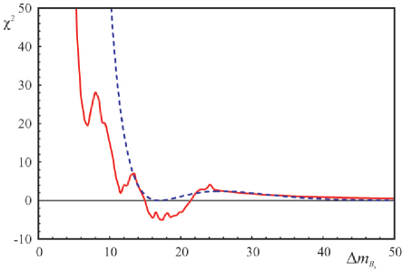
where $\Delta$ is the best estimate according to experiment. The values of $(\Delta,C^{2},\sigma_{t})$ are chosen to give a minimum at $17~{}\rm ps^{-1}$, and a $\chi^{2}$ probability of 5% at $\Delta{m_{B_{s}}}=14.4~{}\rm ps^{-1}$. This function is plotted in Fig. 1, with the $-2\ln{\cal L}_{\infty}(\Delta{m_{B_{s}}})$ curve described earlier superimposed. It may be noted that, in the region of small $\chi^{2}$, the two functions exhibit similar general features. Deviations in the region where both curves have large values don’t matter much — in that region the fit is poor in either case. We have checked the sensitivity of our results to how rapidly the $\chi^{2}$ rises at low values of $\Delta{m_{B_{s}}}$, and find very little effect. Thus, we have some confidence that this empirical treatment is providing dependable answers.

Figure 1: The dashed blue curve is the empirical $\chi^{2}$ expression used to represent the experimental data on $\Delta m_{B_{s}}$ in the fits described in this paper. The solid red curve is an implementation based on the amplitude analysis method; when used in the role of a $\chi^{2}$ term, the function is truncated to non-negative values (see Eqn. (21)).

III.3 Fit results

A “model” ${\cal M}$ and its best-fit solution are kept only if the probability of the fit satisfies $P(\chi^{2}_{\cal M})>P_{min}$, which is typically chosen to be $5\%$. For each “model” ${\cal M}$ accepted, we draw a 95% C.L. contour in the $(\bar{\rho},\bar{\eta})$ plane. The fit is repeated for other “models” ${\cal M}$ by scanning through the complete parameter space specified by a region broad compared with the estimated theoretical uncertainties.

The $\chi^{2}$ minimization thus serves two purposes:

• If a “model” ${\cal M}$ is consistent with the data, we obtain the best estimates for the three CKM parameters, and 95% C.L. contours are determined.

• If a “model” ${\cal M}$ is inconsistent with the data the probability ${\cal P}(\chi^{2}_{\cal M})$ will be low. Thus, the requirement of ${\cal P}(\chi^{2}_{\cal M})_{min}>5\%$ provides a test of compatibility between data and its theoretical description.

If no “model” were to survive we would have evidence of a consistency problem between data and theory, independent of the calculations of the theoretical parameters or the choices of their uncertainties.

III.3.1 Single-parameter sensitivity studies

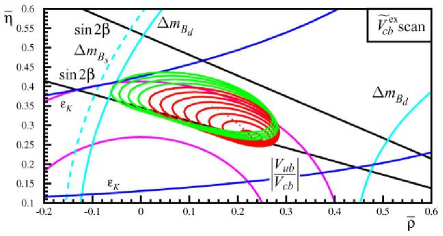
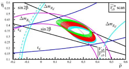
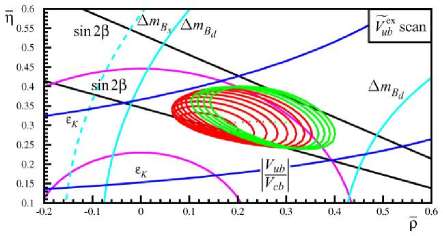
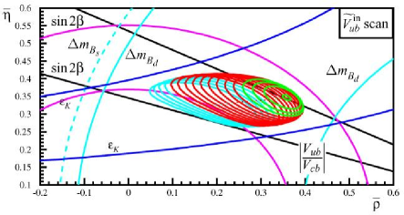
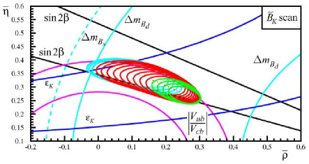
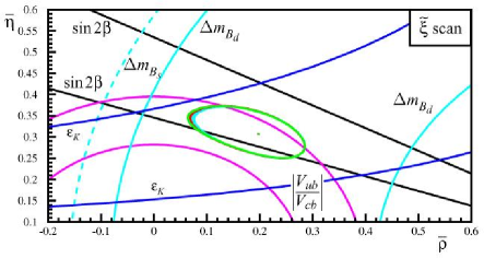
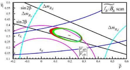
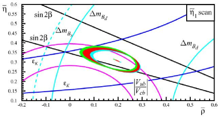
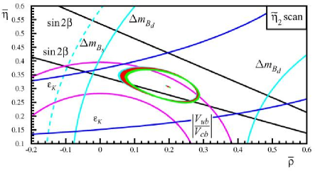
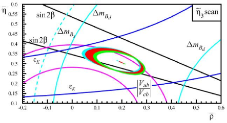
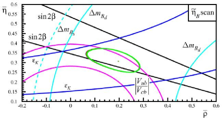
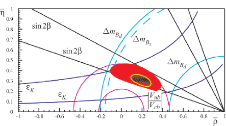
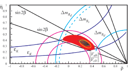
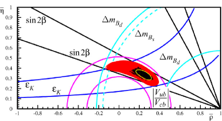
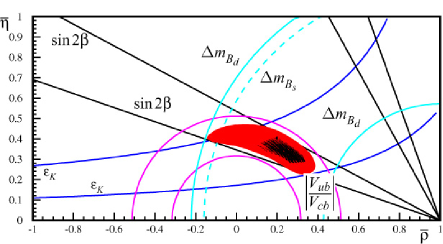
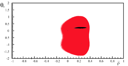
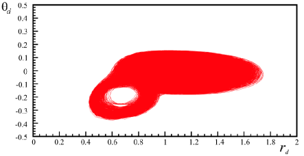
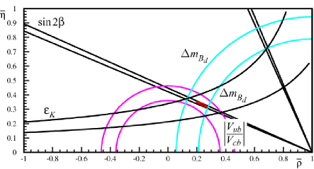
Demonstrating the impact of the different theoretical parameters on the fit results in the $(\bar{\rho},\bar{\eta})$ plane, Figures 2 and 3 show contours for fits in which only one parameter was scanned while the others were kept at their central values. These demonstrate the impact of the model dependence in each of the theoretically uncertain parameters.

In these figures, the red contours correspond to variation of the scanned parameter within its theoretically “allowed” range, while the green and cyan contours result from doubling this range, symmetrically to lower and higher values. The scanned values of the parameter are spaced equidistantly, with nine values covering the central theoretically preferred range and four each the upper and lower extensions. If a fit fails the ${\cal P}(\chi^{2}_{\cal M})_{min}>5\%$ requirement, no contour is drawn.

For qualitative comparison, we show the boundaries of the four bands for $|V_{ub}/V_{cb}|$, $|V_{td}/V_{cb}|$, $\sin 2\beta$, and $\epsilon_{K}$. Since the theoretical parameters are kept at their central values except for the one being varied, the computation of these bands corresponding to the non-varied parameters reflects only experimental uncertainties.

         

         

         

Figure 2: Contours of different models in the $(\bar{\rho},\bar{\eta})$ plane, by varying only one theoretical parameter at a time, left to right, top to bottom: $\widetilde{V}_{cb}^{\rm ex}$, $\widetilde{V}_{cb}^{\rm in}$, $\widetilde{V}_{ub}^{\rm ex}$, $\widetilde{V}_{ub}^{\rm in}$, $\tilde{B}_{K}$, $\tilde{\xi}$, $\widetilde{f_{B}\sqrt{B_{B}}}$. In each case, a total of 17 values were scanned: nine values (red contours) spanning the region $\pm\Delta_{\rm th}$ around the central theoretical value, where $\Delta_{\rm th}$ is the estimated theoretical uncertainty of the parameter; four values (cyan contours) spanning the range from $-2\Delta_{\rm th}$ to $-\Delta_{\rm th}$; and four values (green contours) spanning the range from $\Delta_{\rm th}$ to $2\Delta_{\rm th}$. Note that sometimes fewer than 17 contours appear — this occurs when some of the values of the scanned parameter do not give an acceptable fit (less than 5% $\chi^{2}$ probability).

         

         

Figure 3: Contours of different models in the $(\bar{\rho},\bar{\eta})$ plane, by varying only one theoretical parameter at a time, left to right, top to bottom: $\widetilde{\eta}_{1}$, $\widetilde{\eta}_{2}$, $\widetilde{\eta}_{3}$, and $\widetilde{\eta}_{B}$. The interpretation of the various contours is the same as in Fig. 2.

         

Figure 4: The result of scanning over all theoretically uncertain parameters where: the data from inclusive $|V_{ub}|$ and $|V_{cb}|$ measurements are excluded (left plot), and the data from exclusive $|V_{ub}|$ and $|V_{cb}|$ measurements are excluded (right plot). The black dots show the central values from the fits, and a red contour for each fit indicates the 95% $\chi^{2}$ probability region, according to the experimental (and statistical theoretical) uncertainties.

         

Figure 5: The result of scanning over all theoretical parameters, including information from both inclusive and exclusive measurements of $|V_{ub}|$ and $|V_{cb}|$, with the $\Delta m_{s}$ constraint included in the fit (left) and excluded from the fit (right).

         

Figure 6: The results for fits that include an extra phase, $\theta_{s}$, for the $C\!P$ asymmetry of $B\rightarrow\phi K^{0}_{S}$ (left plot), and for a model-independent analysis that includes an extra scale parameter for $B^{0}_{d}\bar{B}^{0}_{d}$ mixing, $r_{d}$, and an extra phase for the $C\!P$ asymmetry of $B\rightarrow J/\psi K^{0}_{s}$, $\theta_{d}$. Shown are contours in the $\theta_{s}$–$\bar{\rho}$ plane and $\theta_{d}$–$r_{d}$ plane, respectively.

Figure 7: A scan over the allowed range of fits for an envisioned future set of improved experimental and theoretical results.

III.3.2 Scan results in the $\bar{\rho}$–$\,\bar{\eta}$ plane

We now turn to scanning all parameters simultaneously within their theoretically “allowed” ranges. Figures 4 and 5 show the resulting contours for scans in the multi-dimensional model space with some selections on the included experimental information. Note that there is no frequency interpretation for comparing which models are to be “preferred”, other than the statement that at most one model is correct. In this analysis we cannot, and do not, give any relative probabilistic weighting among the contours, or their overlap regions. If we wished to do so, we would proceed to a Bayesian analysis.

From Figure 5 we can determine ranges for the CKM parameters $\bar{\rho}$, $\bar{\eta}$, $A$, and $\lambda$ that are consistent with at least one set of scanned parameters. Table 4 summarizes the present results. The $\pm 1\sigma$ asymmetric experimental errors are shown separately. Furthermore, we obtain ranges for the angles $\alpha$ and $\gamma$, as well as results for $m_{t},\ m_{c}$, and $\beta$ that are consistent with the input values.

III.3.3 Extensions to the standard model

BABAR and Belle have measured the $C\!P$ asymmetry of $B\rightarrow\phi K^{0}_{s}$, yielding a combined value of the sine term in the $C\!P$ asymmetry of $S_{\phi K^{0}_{S}}=-0.39\pm 0.41$ bib:phiks . In the standard model (SM) this should be equal to $\sin 2\beta$ to within $\sim\!4\%$. In models beyond the SM, however, it may differ. The present average deviates from $\sin 2\beta$ by $2.7\sigma$. We can use this result in our fits by adding an additional phase $\theta_{s}$. The resulting set of contours in the $\theta_{s}$–$\bar{\rho}$ plane is shown in Figure 6 (left plot). Presently, the phase is consistent with zero as expected in SM.

Physics beyond the SM may affect $B^{0}_{d}\bar{B}^{0}_{d}$ mixing and $C\!P$ violation in $B\rightarrow J/\psi K^{0}_{s}$ and $B\rightarrow\pi\pi$. Using a model-independent analysis we can add a scale parameter, $r_{d}$, for $B^{0}_{d}\bar{B}^{0}_{d}$ mixing and an additional phase, $\theta_{d}$, for parameterizing the $C\!P$ asymmetry in $B\rightarrow J/\psi K^{0}_{s}$. The SM is then represented by $r_{d}=1$ and $\theta_{d}=0$. The plot on the right-hand side in Figure 6 shows the resulting contours in the $\theta_{d}$–$r_{d}$ plane. With present uncertainties $r_{d}$ and $\theta_{d}$ are consistent with the SM expectations.

In order to extrapolate the $\bar{\rho}$–$\bar{\eta}$ plane in the future, we have assumed that both experimental errors and non-probabilistic theoretical uncertainties are reduced according to projections given in bib:Snowmass2001 . In addition, we have tuned $V_{ub}$ determined from exclusive and inclusive measurements to yield a central value that lies inside the $\sin 2\beta$ band, as with the present central values no fit would survive. The resulting contours in the $\bar{\rho}$–$\bar{\eta}$ plane are shown in Figure 7. In this case several sets of parameters are consistent with the SM. The main constraint is given by $\sin 2\beta$. Measurements of $\gamma$ and $\sin 2\alpha$ are necessary to reduce the range along the $\beta$ rays.

Table 4: Results for selected fit parameters and the angles of the unitarity triangle from the fits in Figure 5. The second and third columns show a lower and upper bound obtained from scanning all theoretical uncertainties. The fourth and fifth columns show the asymmetric experimetal errors obtained from the fits.

Variable	Mean value - $\Delta$	Mean value + $\Delta$	- $\sigma$	$+\sigma$
$\bar{\rho}$	0.1029	0.3372	-0.0668	+0.0264
$\bar{\eta}$	0.281	0.409	-0.0203	+0.0337
$A$	0.796	0.847	-0.024	+0.027
$\lambda$	0.2231	0.2251	-0.0032	+0.0032
$m_{t}$	168.4	170.2	-5.04	5.08
$m_{c}$	1.267	1.323	-0.097	0.0969
$\beta$	0.3619	0.4688	-0.0458	+0.108
$\alpha$	1.451	2.0287	-0.290	+0.0941
$\gamma$	0.70598	1.30	-0.05655	+0.144

IV Visualizing the role of theoretical uncertainties

Returning to the idealized scenario discussed above, recall that the results of the scan of CKM fits over the space $T$ include a mapping of the best-fit value of the fit’s consistency statistic as a function of the $T_{\ell}$. This mapping, derived entirely without the use of theoretical knowledge of these parameters, amounts to a summary of our experimental knowledge of them, assuming the general validity of the theoretical framework from which they arise. It includes the effects of any correlations among the $T_{\ell}$ arising from the experimental data.

We can now in principle combine probabilistic and non-probabilistic information in a useful way without any need for convolution over a priori p.d.f.’s or an equivalent procedure: the above mapping, can simply be compared directly with the theoretically calculated values and uncertainties $\Delta_{T_{\ell}}$ for the theoretical parameters.

This is illustrated conceptually, for the case of two parameters, in Figure 8. The curves represent confidence level contours in the space ${T_{1},T_{2}}$ arising from the fit inputs with experimental (and other probabilistic) uncertainties. The straight lines represent the theoretical information and its uncertainties. Our central point is that we hold that such a diagram contains an efficient summary of all the available information (in a two-variable situation), and that one can go no further in distilling down the overall consistency of this information without introducing additional a priori information or value judgments.

Figure 8: Ideogram of the overlap of the theoretical bounds for two parameters $T_{1}$ and $T_{2}$ with a set of confidence levels contours obtained by scanning a fitting procedure, as described in the text, over the space of the parameters. The dashed lines show the nominal central values of the parameters and the solid lines their bounds.

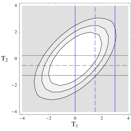
The challenge is to find a comparable way to display and understand the multi-dimensional data set resulting from the actual fits. Ideally, if we could display the entire space, $T$, of the selected parameters at once, no a priori assumptions about theoretical uncertainties would be required at all. The viewer of such a multi-dimensional analog to Figure 8 could see at once the entire set of fits consistent with the experimental data, the effects on this set of the application of the theoretical bounds, and the correlations of these effects among the various parameters.

By adding more dimensions to the display for the output parameters of the fit (e.g., for $\bar{\rho}$ and $\bar{\eta}$), the data could be displayed as a hyperspatial surface in whose shape all the correlations of the fitted CKM parameters with the theoretical inputs would be manifest. Unfortunately, such a plot is beyond normal human ability to visualize directly, so some form of reduction to fewer dimensions is needed.

This makes it necessary, in effect, to integrate over the undisplayed dimensions’ parameters. In order for this to take into account available theoretical information on those parameters, as it must in order to be useful, it is here that a priori bounds or p.d.f.’s must enter. In a Bayesian approach, the integration would be done over an a priori p.d.f. as a true convolution. In a classical frequentist approach the integration in effect becomes a logical OR over all values of the undisplayed parameters that are considered “acceptable”—also an a priori judgement, of course, but a weaker and less specific one than for the Bayesian approach. As noted above, in either approach once the integration is performed the effects of the a priori input tend to be hidden in conventional displays of the fit results.

We have searched for a method that maximizes the amount of simultaneously accessible information while minimizing the use and specificity of a priori inputs, deferring as nearly as possible until the moment of graphical display any convolution of probabilistic and non-probabilistic uncertainties, and thus maintaining a principled separation between these that clearly distinguishes the effects on the CKM fit of any a priori assumptions about the theoretical parameters. The one we have developed is essentially frequentist in its treatment of the projections it makes, which we believe best meets our objectives, though a Bayesian interpretation of projection could also be applied in what follows, mutatis mutandi.

IV.1 Methodology

• Pick two of the parameters $T$ for display. Call these the primary parameters, $T_{1}$ and $T_{2}$.

• Pick a third $T$ parameter, the secondary parameter $T_{s}$. This parameter is singled out for special attention to the effects of projecting over it.

• Call all the other T parameters the undisplayed parameters, $T_{X}$.

• For each point P in the grid of scanned values of $T_{1}\otimes T_{2}$, a number of fits will have been attempted, covering all the scanned values of $T_{s}$ and the $T_{X}$. For each P, evaluate the following hierarchy of criteria against the ensemble of results of these fits, deriving for the point a value we call the “Level”, an integer between 0 and 5 inclusive:

  1. Define a minimum acceptable value of $P(\chi^{2})$. Typically we use 1%, 5%, or 32% for this threshold. Did any of the fits for P pass this cut? If not, assign Level = 0 and stop; otherwise assign Level = 1 and continue.

  2. Did any of the remaining fits lie within the theoretically preferred region for all the undisplayed parameters ${T_{X}}$? If not, stop; if yes, assign Level = 2 and continue.

  3. Did any of the remaining fits have the secondary parameter ${T_{s}}$ within its theoretically preferred region? If not, stop; if yes, assign Level = 3 and continue.

  4. Did any of the remaining fits have ${T_{s}}$ equal to its nominal central value? (That value must have been included in the scan grid for this to make sense.) If not, stop; if yes, assign Level = 4 and continue.

  5. Did any of the remaining fits have all the undisplayed parameters ${T_{X}}$ also at their nominal central values? If not, stop; if yes, assign Level = 5 and stop.

• Now display contours of the quantity Level over the grid in the ${T_{1}}\otimes{T_{2}}$ plane. We assign a unique color to each parameter T, so the contours for ${T_{s}}$ at Level = 3,4 are drawn in the color corresponding to that parameter. The contours for Level = 4,5, which correspond to restrictions of parameters exactly to their central values, are also drawn distinctively, with dashing.

  The Level 3 contour (solid, colored), in particular, displays the allowed region, at the selected confidence level, for ${T_{1}}$ and ${T_{2}}$, based on the experimental data and on limiting all other theoretical parameters to their preferred ranges. Study of the relative spacing of the Level 2, 3, and 4 contours readily reveals the effects of the application of the ${T_{s}}$ bounds on the fit results.

• Overlay the contours with straight lines showing the theoretically preferred ranges and nominal central values for ${T_{1}}$ and ${T_{2}}$, in their respective unique colors, again with dashing for the central value. This allows the theoretical bounds on ${T_{1}}$ and ${T_{2}}$ to be evaluated directly for consistency against all other available data, yet avoiding any convoluted use of priors for these two parameters.

  Comparison of these theoretical bounds for ${T_{1}}$ and ${T_{2}}$ with the Level 3 contour that shows the experimental information, constrained by the application of the theoretical bounds on ${T_{s}}$ and the ${T_{X}}$, allows a direct visual evaluation of the consistency of all available information, with the effects of the application of all theoretical bounds manifest, not obscured by convolutions performed in the fit itself.

• Cyclically permute the set {${T_{1}}$, ${T_{2}}$, ${T_{s}}$} right twice and repeat the previous procedure for the resulting two permutations. Taking all three of the resulting plots together, then, each pair of parameters in the above set will have been used as the primary parameters once, and each parameter will have been used as the secondary once.

• Stitch the three resulting plots together, along their common edges, onto three faces of a cuboid volume and display the result as a three-dimensional image. The consistent use of color allows the effects of the theoretical bounds on all three parameters to be understood together, despite the large amount of information in the plot.

IV.1.1 The basic two-dimensional visualization

We first illustrate the concept with a single two-dimensional plot resulting from the procedure described above. Figure 9 shows the results of this procedure for the standard inputs used in this paper, for simplicity using only exclusive measurements for $|V_{ub}|$ and $|V_{cb}|$. The primary parameters ${T_{1}}$ and ${T_{2}}$ are $\widetilde{B}_{K}$ and $\widetilde{V}_{cb}$, shown in blue and green, respectively. The orthogonal bands show their theoretically preferred ranges and nominal central values.

Figure 9: Contours of the “Level” quantity, defined in the text, in $\widetilde{B}_{K}$ versus $\widetilde{V}_{cb}$, calculated for a global CKM fit. From outside in, the contours are for Level=1) the fit probability cut $P(\chi^{2})>0.32$ (in solid black), 2) restricting the “undisplayed parameters” $\widetilde{\xi}$ and $\widetilde{f_{B}\sqrt{B_{B}}}$ to the ranges $[1.18,1.30]$ and $[211,235]$, respectively (solid black), 3) restricting the “secondary parameter” $\widetilde{V}_{ub}$ to the range $[0.0028,0.0038]$ (solid red), 4) restricting it to its nominal central value of $0.00332$ (dashed red), and 5) similarly restricting $\widetilde{\xi}$ to $1.24$ and $\widetilde{f_{B}\sqrt{B_{B}}}$ to $0.223$ (dashed black). The orthogonal bands show the theoretically preferred ranges and nominal central values for $\widetilde{B}_{K}$ (in blue) and $\widetilde{V}_{cb}$ (in green). The fit uses only information from exclusive measurements of $|V_{ub}|$ and $|V_{cb}|$.

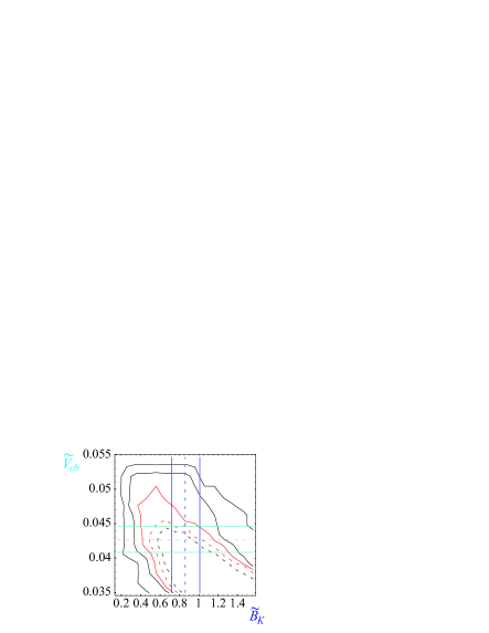
Recall that the symbols $\widetilde{X}$, as previously defined, represent the non-probabilistic part of our lack of knowledge of the true parameters $X$.

The secondary parameter $T_{s}$ is $\widetilde{V}_{ub}$, and the undisplayed scanned parameters $T_{X}$ in this case are $\widetilde{\xi}$ and $\widetilde{f_{B}\sqrt{B_{B}}}$. In this fit, and the others in this section, the QCD $\eta$ parameters are incorporated into the fit with probabilistic uncertainties, not scanned, as a simplification.

We have performed the fits scanned over a grid of all five of these variables, expanded by a factor of five from their theoretically preferred ranges. A strength of the present method is precisely that it permits the ready visualization of the results of going outside the nominal bounds.

The contours enclose successive values of the “Level” quantity, as defined above. The outermost, solid black contour surrounds the region of Level 1, in which fits are required only to pass a $P(\chi^{2})>0.32$ cut; the next, also solid black contour surroundsthe Level 2 region, which now limits fits to those with the “undisplayed parameters” $\widetilde{\xi}$ and $\widetilde{f_{B}\sqrt{B_{B}}}$ within their nominal theoretical ranges. The third contour surrounds the region of Level 3, where the “secondary parameter” $\widetilde{V}_{ub}$ is limited to its nominal range, and is drawn in a solid color, in this case red.

This contour represents our derived experimental knowledge of $\widetilde{B}_{K}$ and $\widetilde{V}_{cb}$ given the theoretical constraints on the other parameters. It can be compared with the theoretical contraints on $\widetilde{B}_{K}$ and $\widetilde{V}_{cb}$, show as the solid colored orthogonal bands. In this case, they overlap perfectly: thus we can see immediately that, given the inputs to these fits, our present experimental constraints on these parameters are strictly less restrictive than the present state of theoretical knowledge.

The dashed contours display the fit results when the theoretical inputs are constrained to their nominal central values; first, at Level 4, for $\widetilde{V}_{ub}$ fixed to $0.00332$, drawn in dashed color, and finally at Level 5 fixing all the remaining parameters ($\widetilde{\xi}$ to $1.24$ and $\widetilde{f_{B}\sqrt{B_{B}}}$ to $0.223$), shown in dashed black. Note the consistent use of dashing to represent central values of the parameters.

The fact that the dashed lines for $\widetilde{B}_{K}$ and $\widetilde{V}_{cb}$ cross within the innermost dashed contour is a representation of the fact that a successful fit ($P(\chi^{2})>0.32$) is obtained even when all the scanned parameters are set to their central values—the set of all the nominal central values is self-consistent.

IV.1.2 The three-dimensional triplet plot

The full power of the method becomes apparent when carrying out the last step in the program described above and considering the three-dimensional plots constructed by assembling the three two-dimensional plots for the pairwise cyclic permutations of a set of three variables. Figure 10a shows the results of this for the same set of variables as in Figure 9; thus, the latter figure appears as one of the faces of the cuboid in Figure 10a.

The consistent use of color and texture coding is important to the comprehension of the plots. Most importantly, in each face of a plot, the colored contours show the effect of the theoretical restrictions on the parameter displayed perpendicularly to it — and the same line styles are used to display the restriction itself on the perpendicular planes.

     

     

     

Figure 10: “Triplet plots”, as defined in the text, for, top to bottom, various sets of three of the five scanned parameters and, left to right, for fits using only exclusive or only inclusive measurements of $|V_{ub}|$ and $|V_{cb}|$. Each triplet plot is a combination of graphs of the kind shown in Figure 9, for all three combinations of a set of three theoretical parameters. The fit probability requirement remains $P(\chi^{2})>0.32$, and the theoretical uncertainty ranges and nominal values are those given elsewhere in the text.

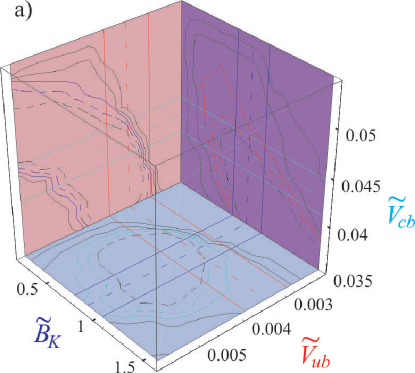
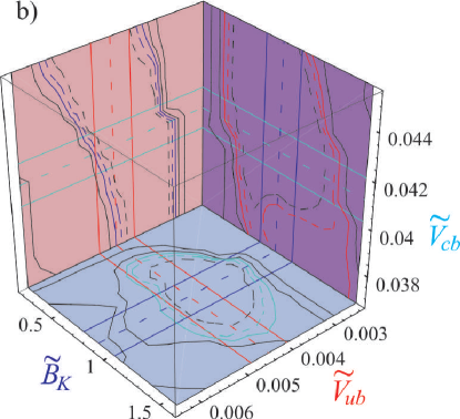
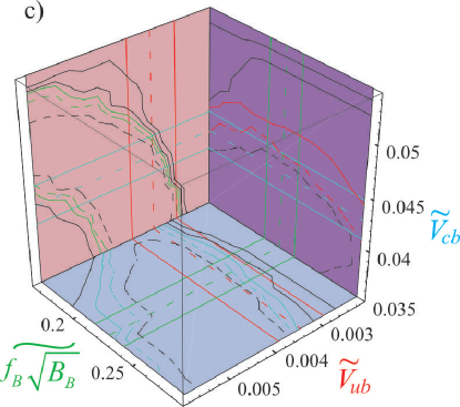
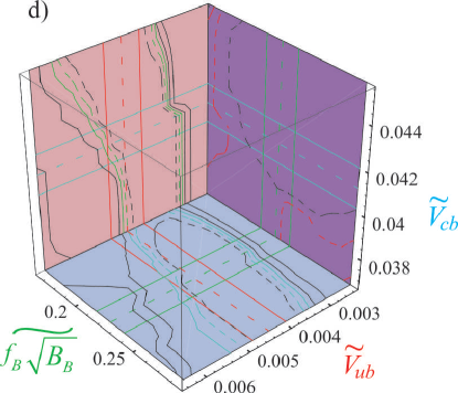
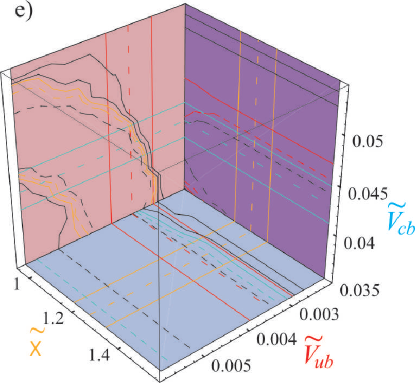
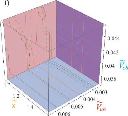
This graphical presentation clearly exhibits the correlations among parameters and measurements. For example, it is possible to tell by inspection in Figures 10a,c,e that experimental data from exclusive measurements is coming to constrain the low side of $|V_{ub}|$ as much as or more than the inputs from theory, with inclusive data similarly constraining the high side.

Further, there is now a region of low $|V_{ub}|$ versus high $|V_{cb}|$ that is excluded on experimental grounds alone, without the need for any of the theoretical inputs here considered. In general, the correlation forced on $|V_{ub}|$ versus $|V_{cb}|$ by the experimental data is readily apparent.

We can observe that $\widetilde{\xi}$ is entirely unconstrained by experimental data within a range more than five times larger than its present theoretical uncertainty. Thus, the theoretical input on $\xi$ is seen to be of particular importance.

$B_{K}$ is seen to be constrained both from above and below by the combination of experimental data and the theoretical input for $|V_{cb}|$, to a region two to three times larger than the present theoretical uncertainty. This can be seen as a measurement of this quantitity, albeit one still dependent on the theoretical input for $|V_{cb}|$.

These are not altogether novel observations — they follow from the structure of the underlying theory, though the details are a quantitative matter — but we believe that this visualization method demonstrates them particularly clearly. It seems a very useful tool in understanding the other CKM analyses, with their typically opaque convolution over the theoretical uncertainties.

It also permits the use of physical judgement in evaluating the meaning of theoretical uncertainties: should a future version of one of these plots reveal an inconsistency of model and data, readers concerned about the role of theoretical uncertainties in that inconsistency could simply read it off a figure, noting that, say, a modest shift in a particular parameter could resolve the discrepancy.

IV.2 Extending to $\bar{\rho}$ and $\bar{\eta}$

The method can be extended to include the Wolfenstein parameters $\bar{\rho}$, $\bar{\eta}$, and $A$, or any other results of the fit, in the visualization of the results. Presentation in terms of $\bar{\rho}$ and $\bar{\eta}$, in particular, permits making a connection with the most common displays resulting from other CKM fitting techniques in the literature, and allows direct visualization of the effects of various theoretical bounds on the values of the Wolfenstein parameters.

However, for each of those parameters that appears in a graph we must remove one of the theoretical parameters into the less readily understood “undisplayed parameters” set and project over it, using some sort of convolution over its assumed distribution. This conflicts with the original rationale for our method, which is to minimize as much as possible the use of hidden a priori information, as in these projections. Thus the extension of these visualization methods to the Wolfenstein parameters represents a compromise between objectives.

With that in mind, the methods we have developed nonetheless can be used to make triplet plots including one, two, or even all three of the Wolfenstein parameters. Since they are outputs of the fit, they are continuous variables and do not form a grid the way the scanned parameters do. We simulate this by rounding them off to a grid—in effect, by binning them—before generating the contours for display.

Because the Wolfenstein parameters do not have independent theoretical bounds that can be used as cuts or displayed in a graphic, they cannot serve exactly as the “secondary parameters” in the scheme as described above. So, when one of them does appear in that position, we treat it as if it were a secondary parameter without any cuts to be applied to it, and show only the Level 1, 2, and 5 contours in the plane to which it is orthogonal. While we also cannot show the solid-color-edged band that we use for theoretical bounds, but we do show a nominal value for each as a colored, dashed line, purely as a guide to the eye.

Figure 11 shows the results of applying this technique to displays of a single theoretical parameter against the two Wolfenstein parameters $\bar{\rho}$ and $\bar{\eta}$, with one plot shown for each of a selection of three of the five theoretical parameters scanned, $\widetilde{B}_{K}$, $\widetilde{V}_{cb}$, and $\widetilde{V}_{ub}$.

In each of the graphs, the $\bar{\rho}$–$\bar{\eta}$ plane displayed at the right rear of the three dimensional volume shows the effects of including only fits with $P(\chi^{2})>0.32$ (outer black countour, Level 1), limiting the graph’s four undisplayed parameters to their theoretical bounds (inner black contour, Level 2), and limiting the graph’s displayed theoretical parameter to its bounds (solid colored contour, Level 3), and to its nominal central value (dashed colored contour, Level 4). The nominal values used for the “guide lines” in the figure are $\bar{\rho}=0.2$ and $\bar{\eta}=0.3$.

     

     

     

Figure 11: “Triplet plots”, as defined in the text, showing the dependence of the fit outputs $\bar{\rho}$ and $\bar{\eta}$ on a single scanned theoretical parameter: from top to bottom, $\widetilde{B_{K}}$, $\widetilde{V_{cb}}$, and $\widetilde{V_{ub}}$, and from left to right, for fits using only exclusive or only inclusive measurements of $|V_{ub}|$ and $|V_{cb}|$. The dashed lines drawn for $\bar{\rho}$ and $\bar{\eta}$ are at purely indicative values of $0.2$ and $0.3$, respectively, and are there only to help guide the eye. The fit probability requirement remains $P(\chi^{2})>0.32$, and the theoretical uncertainty ranges and nominal values are those given elsewhere in the text.

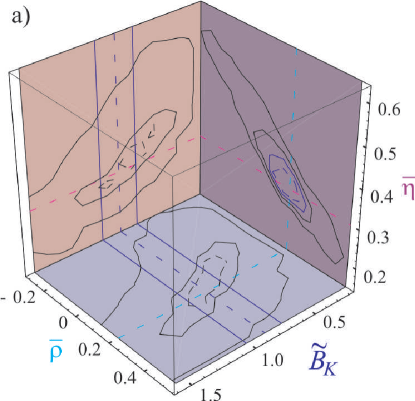
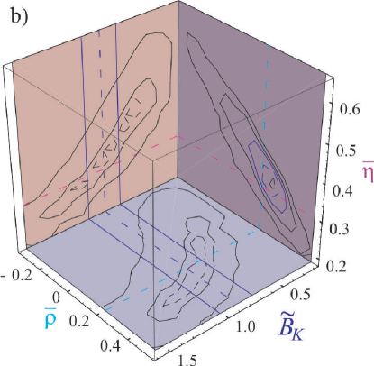
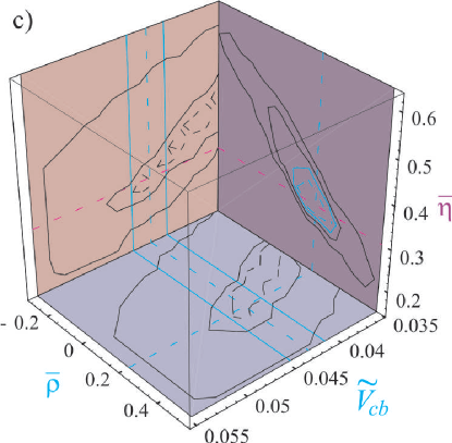
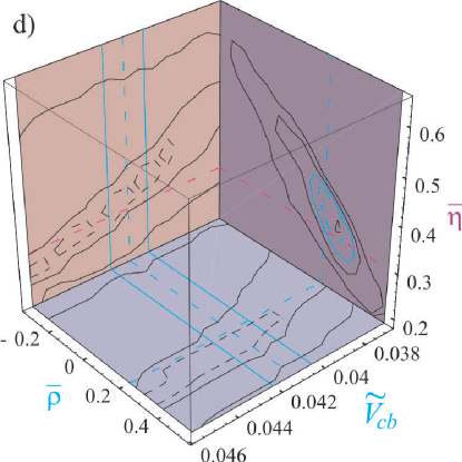
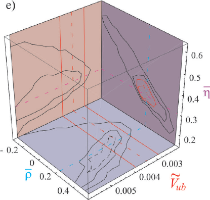
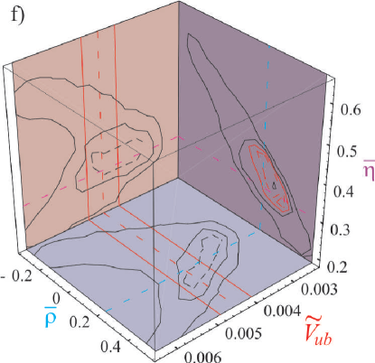
Strikingly clear from these figures is the power and the independence from theoretical inputs of the $\sin 2\beta$ constraint. In each plot in Figure 11 a clear radial band from $(\bar{\rho},\bar{\eta})=(1,0)$ corresponding to this constraint is visible, even for the outermost contour, which reflects scanning over all theoretical ranges enlarged by a factor of five.

Also readily seen is the relative role of the precision of the predictions for each theoretical parameter in constraining $\bar{\rho}$ and $\bar{\eta}$, especially radially. This can be observed by noting the difference in size of the Level 2 (second solid black) and Level 3 (solid color) contours. The former shows the effect of applying our theoretical knowledge of all but the selected parameter, and the latter that of adding to that our knowledge of that parameter.

Thus, for instance, in comparing Figures 11b, 11d, and 11f, based on fits to inclusive $|V_{xb}|$ data, it is easy to see that theoretical input on $\widetilde{B}_{K}$ plays the largest role in constraining $\bar{\rho}$ and $\bar{\eta}$, while the theoretical input for $\widetilde{V}_{cb}$ (for inclusive measurements) has little effect once the other theoretical parameters have been determined. (The corresponding plots, not included here, for $\widetilde{f_{B}\sqrt{B_{B}}}$ and $\widetilde{\xi}$ show that they have comparatively small roles as well.)

V Conclusion and Future directions

This work is already beginning to shed light on the sensitivity of CKM fits to assumptions regarding the parameterization of theoretical uncertainties. We believe that in the future it will become a valuable tool for understanding the results of such fits and for assessing whether, in fact, inconsistencies with the standard model may have emerged as the precision and breadth of measurements are improved.

By clearly separating the probablistic uncertainties associated with measured quantitities from the a priori unknown distributions of theoretical quantities, we have attempted to expose the effects of assumptions about the distribution of theoretical uncertainties on the results of fits that purport to extract a statistic representing the degree of “self-consistency” of the CKM sector of the standard model. In particular, the clear correlation found between “best-fit” values for $\bar{\rho}$ and $\bar{\eta}$ and the theoretical inputs for $B_{K}$ and the computations of $|V_{cb}|$, which are quite model dependent, should prompt a cautious approach in future attempts to ascertain the degree of consistency of unitarity triangle-based investigations of the CKM matrix.

The existence of such correlations demonstrates the dangers of constructing contours covering a range of values of theoretically uncertain parameters that may then be interpreted as contours of equal probability.

In the next decade, as lattice calculations of many of the theoretical quantities that enter into CKM unitarity triangle studies improve and gain control of systematic uncertainties, it will be possible to assign a probability distibution function to theoretical uncertainties in a principled manner. Until we reach this nirvana, however, an explicit display of the effect of the (unknown) distribution of theoretical errors on conclusions about the validity of the standard model will remain important.

References

- (1) The BABAR Physics Book, BABAR Collaboration, (P.F. Harrison and H.R. Quinn, eds.). SLAC-R-0504, 1998.
- (2) M. Ciuchini, G. D’Agostini, E. Franco, V. Lubicz, G. Martinelli, F. Parodi, P. Roudeau and A. Stocchi, CKM Triangle Analysis: A Critical Review with Updated Experimental Inputs and Theoretical Parameters, J. High Energy Physics 107, 13, 2001.
- (3) A. Höcker, H. Lacker, S. Laplace and F. Le Diberder , A New Approach to a Global Fit of the CKM Matrix, Eur. Phys. J. C 21, 225, 2001.
- (4) Proceedings of the Workshop on the CKM Unitarity Triangle, CERN, February 2002 (in preparation; ephemera available at http://ckm-workshop.web.cern.ch/).
- (5) L. Wolfenstein, Phys. Rev. Lett. 51, 1945, 1983.
- (6) A. J. Buras, M. E. Lautenbacher, and G. Ostermaier, Phys. Rev. D 50, 3433, 1994.
- (7) R.A. Briere, CLEO collaboration, hep-ex/0203032.
- (8) K. Abe et al (BELLE collaboration), Phys.Lett. B 526, 247 (2002).
- (9) D. Abbaneo et al. ( LEP working group), (2002).
- (10) M.E. Luke, Phys. Lett. B 252, 447 (1990).
-
(11)
A. Czarnecki, Phys. Rev. Lett. 76, 4124 (1996);
A. Czarnecki and K. Melnikov Nucl. Phys. B505, 65 (1997). -
(12)
M. Neubert, Phys. Lett. B 338, 84 (1994);
C.G. Boyd and I.Z. Rothstein, Phys. Lett. B 395, 96 (1997). -
(13)
A. Czarnecki, K. Melnikov and N.G. Uraltsev,
Phys. Rev. D 57, 1769 (1998);
N.G. Uraltsev, UND-HEP-00-BIG07 (hep-ph/0010328), (2000). - (14) J.N. Simone et al. Nucl. Phys. Proc. Suppl. 83 334 (2000).
- (15) S. B. Athar et al. (CLEO Collaboration), hep-ex/0304019.
- (16) N. Isgur, D. Scora, B. Grinstein, and M.B. Wise, Phys. Rev. D 39, 799 (1989); N. Isgur and D. Scora, Phys. Rev. D 52, 2783 (1995); M. Beyer and N. Melikhov, Phys. Lett. B 416, 344 (1998); L. del Debbio et al., Phys. Lett. B 416, 392 (1998); P. Ball and V. M. Braun, Phys. Rev. D 58, 094016 (1998); Z. Ligeti and M.B. Wise, Phys. Rev. D 53 4937 (1996); E.M. Aitala et al., Phys. Rev. Lett. 80, 1393 (1998).
- (17) N. Uraltsev et al., Eur. Phys. J. C 4, 453 (1998); A. Hoang et al., Phys. Rev. D59, 074017 (1999); N. Uraltsev, Int.J.Mod.Phys.A 14, 4641 (1999); I. Bigi hep-ph/9907270.
- (18) T. Inami and C.S. Lim, Prog. Th. Phys. 65, 297 (1981).
- (19) S. Herrlich and U. Nierste, Nucl. Phys. B419, 292, (1994).
- (20) A.J. Buras, M. Jamin and P.H. Weisz, Nucl. Phys. B347, 491 (1990).
- (21) S. Herrlich and U. Nierste, Phys. Rev. D 52, 6505 (1995); Nucl. Phys. B476, 27 (1996).
- (22) M.P. Jimack and H.G. Moser, Nucl. Instr. Meth. A408, 36 (1998).
- (23) B. Aubert et al., hep-ex/0203007 (2002).
- (24) T. Higuchi et al., hep-ex/0205020 (2002).
- (25) T. Affolder et al. (CDF collaboration) Phys.Rev. D 61, 072005 (2000).
- (26) R. Barate et al. (ALEPH collaboration), Phys. Lett. B 492, 259 (2000).
- (27) C. O. Dib, et al., Phys. Rev. D 41, 1522 (1990).
- (28) V. Andreev et al., Summary of mixing working group, http://lepbosc.web.cern.ch/LEPBOSC/ (2002); D. Abaneo et al. cern-ep-2001-050 (2001).
- (29) K. Hagiwara et al., Phys. Rev. D 66, 010001 (2002).
- (30) Proceedings of the 18th International Symposium, Lattice 2000, Bangalore, T. Bhattacharya, R. Gupta and A. Patel, eds., Nucl. Phys. Proc. Suppl. 94 (2001).
- (31) A. Bornheim et al. (CLEO collaboration), Phys. Rev Lett. 88, 231813 (2002).
- (32) B. Aubert et al. (BABAR collaboration), hep-ex/0207081 (2003).
- (33) B. Aubert et al. (BaBar Collaboration), Phys. Rev. Lett. 90 181810 (2003).
- (34) M. Artuso, FPCP Conference, June 3-6, 2003, Paris.
- (35) K. Hagiwara et al., http://pdg.lbl.gov/ (2003).
- (36) Computed by G.E. from experimental results quoted by M. Calvi, FPCP Conference, June 3-6, 2003, Paris and M. Artuso, FPCP Conference, June 3-6, 2003, Paris.
- (37) M. Battaglia et al. ( LEP working group), (2002).
- (38) F. Parodi, personal communication (2002); M. Ciuchini et al. op. cit..
- (39) M. Battaglia, et al. Proceedings of the Workshop on the CKM Unitarity Triangle, CERN, 13-16 February 2002, hep-ph/0304132.
- (40) B. Aubert et al.(BABAR Collaboration), Proceedings of the XXXI International Conference on High Energy Physics, Amsterdam, 2002, hep-ex/0207070. K. Abe et al. (Belle Collaboration), Phys. Rev. D. 67, 031102R (2003).
- (41) P.Burchat et al., Physics at a Asymmetric Factory, in Proceedings of the APS/DPF/DPB Summer Study on the Future of Particle Physics (Snowmass 2001), Snowmass, Colorado. eConf C010630:E214,2001.