Balance functions in coalescence model

Abstract

It is shown that the quark-antiquark coalescence mechanism for pion production allows to explain the small pseudorapidity width of the balance function observed for central collisions of heavy ions, provided effects of the finite acceptance region and of the transverse flow are taken into account. In contrast, the standard hadronic cluster model is not compatible with this data.

1. Recently, measurements of balance functions [2] in central collisions of heavy ions were reported by the STAR collaboration [3]. The striking feature observed in the data is the small width of the balance functions (in rapidity and in pseudorapidity), as compared to the expectations from the expanding thermally equilibrated quark-gluon plasma [4]. This indicates that hadronization occurs only at the very late stage of the development of the system [5].

One may then ask if the hadronization properties of the system produced in central collisions of heavy ions (as reflected in the balance function) are similar to those observed in nucleon-nucleon collisions. To investigate this problem we have evaluated the expected width of the balance function in pseudorapidity, using the pion cluster model which some time ago was successfully applied to nucleon-nucleon data [6]. Corrections due to the finite acceptance region of [3] and the effects of the transverse flow were included.

Our estimates show that to obtain consistency with the data of [3] for central collisions, the decay width of the pion cluster (in its rest frame) must be substantially narrower than that corresponding to isotropic decay. Thus one must conclude that the hadronization of the system produced in heavy ion collisions is rather different from that produced in hadronic collisions, where isotropic clusters can approximately account for the data [6].

Looking for a more adequate description, we considered the coalescence model [7], which we generalized to include correlations. We thus assume that the hadronization proceeds in three steps. First, partons form neutral clusters. Subsequently, each cluster decays into some number of gluons and one $q\bar{q}$ pair (either $u\bar{u}$ or $d\bar{d}$). Quarks and antiquarks then recombine into positive, negative and neutral pions. The remaining gluons form new clusters and the process is continuing until all partons are transformed into hadrons.

We show that this generalized coalescence model gives a good description of the data from [3], provided the decay of clusters into quarks and antiquarks is isotropic, which seems a rather natural assumption. The obtained reduction of the width of the balance function (essential to account for the data) is a natural consequence of the coalescence process. It follows simply from the fact that the dispersion of the average of two independent random variables is smaller than the dispersion of each of them by factor $\sqrt{2}$.

It should be emphasized that we are discussing here only the angular distributions (expressed in terms of pseudorapidity). The natural assumption of approximately isotropic and uncorrelated cluster decay is then sufficient to describe the width of the balance function. This is not the case for rapidity distribution where more detailed information on cluster decay is needed.

Our conclusion is that the generalized coalescence model provides a natural explanation of the very narrow width of the balance function observed in [3]. This result is a consequence of a very general fenomenon, characteristic for coalescence mechanism and thus, in our opinion, it does not depend on details of the specific structure of correlations between partons proposed in this note. Since, as we have seen, the model based solely on hadronic degrees of freedom is not adequate, we feel that our result provides a rather strong argument in favour of the coalescence scenario.

2. The balance functions can be expressed in terms of the single and double particle densities [4, 8]. Assuming, for simplicity, the $(+-)$ symmetry we have

$$B(\Delta_{2}|\Delta_{1})=D(-,\Delta_{2}|+,\Delta_{1})-D(+,\Delta_{2}|+,\Delta_{1})$$ (1)

with

$$D(+,\Delta_{2}|+,\Delta_{1})=D(-,\Delta_{2}|-,\Delta_{1})=\frac{\int_{\Delta_{2}}d\eta_{2}\int_{\Delta_{1}}d\eta_{1}\frac{d^{2}n_{++}}{d\eta_{1}d\eta_{2}}}{\int_{\Delta_{1}}d\eta_{+}\frac{dn_{+}}{d\eta_{+}}}$$ (2)

$$D(-,\Delta_{2}|+,\Delta_{1})=D(+,\Delta_{2}|-,\Delta_{1})=\frac{\int_{\Delta_{2}}d\eta_{2}\int_{\Delta_{1}}d\eta_{1}\frac{d^{2}n_{+-}}{d\eta_{1}d\eta_{2}}}{\int_{\Delta_{1}}d\eta_{+}\frac{dn_{+}}{d\eta_{+}}}$$ (3)

where $dn/d\eta$ and $dn/d\eta_{1}d\eta_{2}$ are the corresponding particle densities in pseudorapidity.

The measurements of STAR require both particles to be in an interval $-\Delta\leq\eta_{1},\eta_{2}\leq\Delta$ (acceptance) while the difference of (pseudo)rapidities is kept fixed. This suggests a change of variables:

$$\eta_{1}-\eta_{2}=\delta;\;\;\;\;(\eta_{1}+\eta_{2})/2=z.$$ (4)

The integrations must be performed over $dz$ with $\delta$ being fixed. This implies that $z$ must be kept inside the interval $-\bar{\Delta}\leq z\leq\bar{\Delta}$ where $\bar{\Delta}=\Delta-|\delta|/2$.

Thus the balance function measured in [3] is given by

$$B_{s}(\delta;\Delta)=\frac{\int_{-\bar{\Delta}}^{-\bar{\Delta}}dz\left[d^{2}n_{+-}/dzd\delta-d^{2}n_{++}/dzd\delta\right]}{\int_{-\Delta}^{+\Delta}d\eta_{+}dn_{+}/d\eta_{+}}$$ (5)

3. Consider first a model in which pions are produced in neutral, isotropic clusters. It is well known that such models can account for the gross features of the nucleon-nucleon data [6]. The distribution of clusters is denoted by $\rho_{c}(Y)$ where $Y$ is the cluster pseudorapidity.

To simplify the problem we assume that clusters decay into two charged particles and any number of neutrals.

The distribution in cluster decay is

$$\frac{dN_{+-}}{d\eta_{+}d\eta_{-}}=h(z-Y)f(\eta_{+}-Y)f(\eta_{-}-Y)$$ (6)

where $h(z-Y)$ is responsible for correlations: $h\equiv 1$ if the decay products are uncorrelated.

The single particle distribution in cluster decay $\rho(\eta_{+}-Y)$ is obtained by integration of (6) over rapidity of one particle. Both distributions are normalized to unity.

The distribution of all particles is the convolution

$$\frac{dn_{+}}{d\eta_{+}}=\int dY\rho_{c}(Y)\rho(\eta_{+}-Y)$$ (7)

with identical formula for negative particles.

To evaluate the two-particle distributions one has to take into account that some pairs may come from different clusters and some others from one cluster. As is well-known (and can be easily confirmed by explicit calculation) the contribution from different clusters cancels in the balance function and thus only $(+-)$ pairs from one cluster do contribute. Their distribution is given by

$$\frac{d^{2}n_{+-}}{d\eta_{+}d\eta_{-}}=\int dY\rho_{c}(Y)h(z-Y)f(\eta_{+}-Y)f(\eta_{-}-Y).$$ (8)

Introducing (8) into (5) we have

$$B(\delta;\Delta)=\frac{\int_{-\bar{\Delta}}^{+\bar{\Delta}}dz\int dY\rho_{c}(Y)h(z-Y)f(\eta_{+}-Y)f(\eta_{-}-Y)}{\int_{-\Delta}^{\Delta}d\eta\int dY\rho(\eta-Y)}.$$ (9)

4. To continue, we perform a simple exercise, assuming that all functions are Gaussians. We take

$$\rho_{c}(Y)=\frac{<N_{c}>}{A\sqrt{\pi}}\exp(-Y^{2}/A^{2});\;\;\;$$

$$f(u)=\frac{1}{f\sqrt{\pi}}\exp(-u^{2}/f^{2});\;\;\;\;h(u)=\sqrt{1+f^{2}/2g^{2}}\exp(-u^{2}/g^{2})$$ (10)

Using (10) one can evaluate the single particle distribution in cluster decay:

$$\rho(\eta)=\frac{1}{a\sqrt{\pi}}\exp(-\eta^{2}/a^{2});\;\;\;a=f\frac{\sqrt{1+f^{2}/4g^{2}}}{\sqrt{1+f^{2}/2g^{2}}}.$$ (11)

This gives

$$\frac{dn_{+}}{d\eta_{+}}=\frac{<N_{c}>}{\sqrt{\pi(A^{2}+a^{2})}}\exp[-\eta_{+}^{2}/(A^{2}+a^{2})];$$

$$\int dY\rho_{c}(Y)h(z-Y)f(\eta_{1}-Y)f(\eta_{2}-Y)=$$

$$=<N_{c}>\frac{1}{f\sqrt{2\pi}}\exp(-\delta^{2}/2f^{2})\frac{1}{F\sqrt{\pi}}\exp(-z^{2}/F^{2})$$ (12)

with

$$F^{2}=\frac{f^{2}+2A^{2}[1+f^{2}/2g^{2}]}{2[1+f^{2}/2g^{2}]}$$ (13)

This result introduced into (9) allows to express the integrals over $z$ and $y$ in terms of the error function. The result is

$$B(\delta;\Delta)=\frac{1}{f\sqrt{2\pi}}\exp(-\delta^{2}/2f^{2})\frac{erf[(\Delta-|\delta|/2)/F]}{erf[\Delta/\sqrt{A^{2}+a^{2}}]}$$ (14)

which completes the calculation.

This exercise shows that -in the limit of large acceptance- the width of the balance function is determined by the parameter $f$ which describes the cluster decay.

5. These results can be used to evaluate expectations from isotropically decaying clusters which were found roughly compatible with the data on hadron-hadron collisions [6]. In this case the cluster decay distribution is

$$\rho(\eta)=\frac{1}{2(\cosh\eta)^{2}}$$ (15)

giving the cluster decay width $<|\eta|>=\log 2$. This can be approximated by a Gaussian of the form (11) with $a=\log 2\sqrt{\pi}\approx 1.23$. Ignoring for the time beeing the effect of finite acceptance, we thus conclude from (11) that the expected width of the balance function $<|\delta|>$ must be larger than $a\sqrt{2}/\sqrt{\pi}\approx.98$ and thus by far exceeds the one measured in [3].

Finite acceptance [$\Delta=1.3$] of the STAR measurements [3] reduces the observed width of the balance function, as seen from (14). This is not sufficient, however, to bring the data in agreement with the model of isotropic pion clusters. The width $<|\delta|>$ calculated from (11) for isotropic clusters with $f/g=0$ (uncorrelated dcay) equals 0.67 at $A=3.5$ (this value of $A$ is roughly consistent with data for central collisions [9]), and does not change significantly when $A$ varies around this value. Since, furthermore, $<|\delta|>$ increases with increasing $f/g$, there is no chance to meet the experimental value of $0.55$.

Another effect which may be responsible for the small width of the balance function is the transverse flow. Indeed, the clusters which are isotropic in their rest frame will not appear isotropic when moving with a transverse velocity. As shown in [10], the distribution (15) is then -to a good approximation- replaced by

$$\rho(\eta)=\frac{1}{2\cosh^{2}\eta}\frac{\cosh Y_{\perp}}{[1+\sinh^{2}Y_{\perp}\tanh^{2}\eta]^{3/2}}$$ (16)

where $Y_{\perp}$ is the transverse rapidity, $Y_{\perp}=0.5\log[(1+v)/(1-v)]$, and $v$ is the tranverse velocity of the cluster.

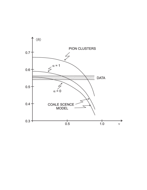
Figure 1: Width of balance function versus velocity of transverse flow.

We have calculated the width of the balance function with (16) approximated by a Gaussian of the same width as that of (16). The results are shown in Fig.1 where $<|\delta|>$ is plotted versus $v$, for $A=3.5$. The measured values for most central events (as reported in [3]) are also indicated. One sees that the calculated width decreases with increasing transverse velocity of clusters. One also sees that to obtain quantitative agreement with data the transverse velocity must approach $0.8c$. Such a large value seems difficult to reconcile with other estimates of the transverse velocity [11].

6. The pion cluster model discussed so far ignores entirely the parton structure of the final system of hadrons. One may therefore not be surprized that it fails to describe the data from central heavy ion collisions. This argument suggests to try a model in which the parton structure is built in from the beginning. To this end we investigated coalescence model [7] which we generalized to include the correlations inside the system.

To introduce correlations we assume that -just before hadronization- the QGP forms the weakly correlated neutral clusters. The clusters decay into quarks⁴, antiquarks and gluons. One cluster provides one³ $q\bar{q}$ pair (either $u\bar{u}$ or $d\bar{d}$) and any number of gluons. In the final step quarks and antiquarks coalesce into observed hadrons. The remaining gluons form again neutral clusters and the process continues.

Thus the model we consider is basically the well-known coalescence model [7] supplemented by a prescription for correlations. Since the coalescence model was rather succesful in description of single particle spectra in central collisions of heavy ions [7, 12], it seems worthwhile to investigate its extention to correlation phenomena (see also [13]). Admittedly, the proposed extension is very simple - perhaps even simplistic. It contains, however, all ingredients necessary to formulate and study the width of balance functions which is of interest in this paper. Therefore we do not find necessary at the moment to formulate and discuss a more general and/or detailed approach.

7. To evaluate the balance function we need the distribution of pairs of charged pions, same charge as well as opposite charge. The pairs of same charge can be constructed by coalescence of the decay products of four clus-ters (two U-clusters and two D-clusters). The distribution of the pairs of opposite charge consists of two terms: one identical to the distribution of same charge pairs and another one, arizing from coalescence of the decay products of two clusters (one U-cluster and one D-cluster). Thus the contributions involving four clusters exactly cancel and we only have to consider the distribution of pions of opposite charge which result from coalescence of decay products of one U-cluster and one D-cluster.

This distribution can be expressed as

$$\rho(\eta_{+},\eta_{-})=\int dY_{U}dY_{D}\rho_{G}(Y_{C},\Delta_{Y})$$

$$\int d\eta_{u}d\eta_{\bar{u}}f_{q}(\eta_{u}-Y_{U})f_{q}(\eta_{\bar{u}}-Y_{U})h_{q}([\eta_{u}+\eta_{\bar{u}}]/2-Y_{U})$$

$$\int d\eta_{d}d\eta_{\bar{d}}f_{q}(\eta_{d}-Y_{D})f_{q}(\eta_{\bar{d}}-Y_{D})h_{q}([\eta_{d}+\eta_{\bar{d}}]/2-Y_{D})$$

$$\delta[\eta_{+}-(\eta_{u}+\eta_{\bar{d}})/2]\delta[\eta_{-}-(\eta_{d}+\eta_{\bar{u}})/2]\Phi[\eta_{u}-\eta_{\bar{d}}]\Phi[\eta_{d}-\eta_{\bar{u}}]$$ (17)

where $f_{q}$ and $h_{q}$ are responsible for the distribution of quarks in decay of either $U$ or $D$ cluster, while $\Phi$ summarizes the properties of the coalescence process. Finally, $\rho_{G}(Y_{C},\Delta_{Y})$ denotes the joint distribution of $U$ and $D$ clusters with average rapidity $Y_{C}$, where

$$Y_{C}=\frac{Y_{U}+Y_{D}}{2};\;\;\;\;\Delta_{Y}=Y_{U}-Y_{D}$$ (18)

To simplify the discussion, in the following we shall assume that $\rho_{G}$ factorizes:

$$\rho_{G}(Y_{C},\Delta_{Y})=\rho_{C}(Y_{C})\rho(\Delta_{Y})$$ (19)

Taking advantage of the delta functions we can rewrite (17) as

$$\rho(\eta_{+},\eta_{-})=\int dY_{C}d\Delta_{Y}\rho_{G}(Y_{C},\Delta_{Y})\int du_{+}du_{-}$$

$$f_{q}\left(\eta_{+}+\frac{u_{+}}{2}-Y_{C}\right)f_{q}\left(\eta_{-}+\frac{u_{-}}{2}-Y_{C}\right)h_{q}\left(z+\frac{u_{+}+u_{-}}{4}-Y_{C}\right)$$

$$f_{q}\left(\eta_{-}-\frac{u_{-}}{2}-Y_{C}\right)f_{q}\left(\eta_{+}-\frac{u_{+}}{2}-Y_{C}\right)h_{q}\left(z-\frac{u_{+}+u_{-}}{4}-Y_{C}\right)$$

$$\Phi\left(u_{+}+\Delta_{Y}\right)\Phi\left(u_{-}+\Delta_{Y}\right)$$ (20)

where $z=(\eta_{+}+\eta_{-})/2$.

To proceed, we again consider Gaussians

$$f_{q}(x)=\frac{1}{c\sqrt{\pi}}e^{-x^{2}/c^{2}};\;\;\;h_{q}(x)=\sqrt{1+a^{2}/2h^{2}}\exp[-x^{2}/h^{2}]$$

$$\Phi(x)=\frac{1}{p\sqrt{\pi}}e^{-x^{2}/p^{2}}.$$ (21)

With this Ansatz, the integrals over $du_{+}du_{-}$ can be performed. The result is

$$\rho(\eta_{+},\eta_{-})=Ce^{-\delta^{2}/c^{2}}\int dY_{C}\rho_{C}(Y_{C})\exp\left[-\frac{4\left[z-Y_{C}\right]^{2}}{c^{2}}(1+c^{2}/2h^{2})\right]$$ (22)

where $\;\delta=\eta_{+}-\eta_{-}\;$ and $C$ is a constant, irreleveant for further discussion.

The formula (22) can be now introduced into (5) and thus the balance function can be calculated. In the limit of very large acceptance we obtain

$$B_{s}(\delta;\Delta)_{\Delta\;\rightarrow\;\infty}=\frac{1}{c\sqrt{\pi}}e^{-\delta^{2}/c^{2}}$$ (23)

One sees that -in this limit- the width of the balance function depends on one parameter which -to a large degree- determines also the distribution in decay of a cluster into free quark and antiquark. Indeed, using (17) and (21), one can show that the decay distribution in the rest frame of the cluster is given by

$$\rho_{p}(\eta_{u})=\frac{1}{d\sqrt{\pi}}\exp\left[-\frac{\eta_{u}^{2}}{d^{2}}\right]$$ (24)

where

$$d^{2}={c^{2}}\frac{1+c^{2}/4h^{2}}{1+c^{2}/2h^{2}}.$$ (25)

8. It seems natural to assume that -in their rest frame- clusters decay isotropically. This means that their decay distribution is given by (15), the same as for the clusters of pions considered before. It follows that -for an uncorrelated decay ($c/h\approx 0$)- the parameters $f$ in (10) and $c$ in (21) are identical. Comparing (14) and (23) we thus conclude that in the coalescence model the width of the balance function is expected to be by factor $\sqrt{2}$ smaller than that obtained for pion clusters. The reason is clear: the dispersion of the pion rapidity is reduced by precisely this factor when the pion is formed by random coalescence of a quark and an antiquark.

Repeating the argument of the section 5, we thus conclude that -ignoring for the moment the corrections for finite acceptance and effects of transverse flow- the width of the balance function is expected to lie between .69 and .98 (the lower limit is obtained for $\alpha=(c/h)^{2}=0$, i.e. when the decay products of a cluster are uncorrelated).

To compare this result with the data we have to estimate the corrections. To this end we take the Gaussian Ansatz for $\rho_{C}$:

$$\rho_{C}(Y_{C})=\frac{1}{A\sqrt{\pi}}e^{-Y_{C}^{2}/A^{2}}$$ (26)

which allows to evaluate explicitely the integrals in (22). We obtain

$$B_{s}(\delta;\Delta)=\frac{1}{c\sqrt{\pi}}e^{-\delta^{2}/c^{2}}\frac{erf[2(\Delta-|\delta|/2)/b]}{erf[2\Delta/\sqrt{b^{2}+c^{2}}]}$$ (27)

where

$$b^{2}=\frac{c^{2}+4A^{2}(1+c^{2}/2h^{2})}{1+c^{2}/2h^{2}}$$ (28)

Using (27) one can now follow the argument of section 5 and evaluate the width of the balance function, taking into account the finite acceptance and the transverse flow. In Figure 1 the width of the balance function evaluated from (27) is plotted versus $v$ for $A=3.5$ and two values of the parameter $\alpha=c^{2}/h^{2}$. One sees that these effects reduce substantially the calculated width. The value found in [3] for central collisions is reproduced with transverse velocity below 0.5, consistent with other estimates of the transverse flow [11].

One also sees from the Fig. 1 that in the coalescence model the calculated width is smaller than the value 0.65 found in [3] for peripheral collisions. This is not surprizing: in peripheral collisions a substantial part of the particle production should resemble the elementary nucleon-nucleon collisions which are not expected to follow the coalescence mechanism [12] and are characterized by a significantly larger width of the balance function [2, 6]. As seen from Fig.1, the width of the balance function calculated from the pion cluster model (adequate for nucleon-nucleon collisions) is indeed close to 0.65.

9. In conclusion, we have shown that the coalescence mechanism implies a substantial reduction of the pseudorapidity width of the balance function. This allows to explain the small width observed for central collisions of heavy ions [3], provided the corrections due to the finite acceptance region and to the transverse flow are taken into account. This result supports the coalescence mechanism as the final stage of the process of hadronization.

Acknowledgements

Thanks are due to W.Broniowski, W. Florkowski and K. Zalewski for comments and encouragement. This investigation was supported in part by the by Subsydium of Foundation for Polish Science NP 1/99 and by the Polish State Commitee for Scientific Research (KBN) Grant No 2 P03 B 09322.

References

- [1]
- [2] See, e.g., D.Drijard et al., Nucl.Phys. B155 (1979) 269; Nucl. Phys. B166 (1980) 233.
- [3] STAR coll., J.Adams et al., Phys. Rev. Lett. 90 (2003) 172301.
- [4] S.A.Bass, P.Danielewicz and S.Pratt, Phys. Rev. Lett. 85 (2000) 2689.
- [5] S.Pratt,Nucl. Phys. A698 (2002) 531c; Nucl.Phys. A715 (2003) 389c.
- [6] For a review, see L. Foa, Phys. Rept. 22 (1975) 1.
- [7] T.S.Biro, P.Levai and J.Zimanyi, Phys. Lett. B347 (1995) 6; J.Zimanyi, P.Levai and T.S.Biro Heavy Ion Phys. 17 (2003) 205 and references quoted there; J.Pisut, N.Pisutova, Acta Phys. Pol. B28 (1997) 2817; R.Lietava and J. Pisut, Eur. Phys. J. C5 (1998) 135.
- [8] S.Jeon and S.Pratt, Phys. Rev. C65 (2002) 044902; T.Trainor, hep-ph/0301122; S.Jeon and V.Koch, hep-ph/0304012.
- [9] PHOBOS coll., B.B.Back et al., Phys.Rev.Lett 87 (2001) 102303; G.S.F. Stephans et al., Acta Phys. Pol. B33 (2002) 1419; BRAHMS coll., I.G.Bearden etal., Phys.Lett. B523 (2001) 227; P.Staszel et al., Acta Phys. Pol. B33 (2002) 1387.
- [10] K.Zalewski, Acta Phys. Pol. B9 (1978) 87.
- [11] See, e.g., G.Van Buren, Nucl. Phys. A715 (2003) 129c; T.Chujo, Nucl.Phys. 715 (2003) 151c; W.Broniowski, A.Baran and W.Florkowski, Acta Phys.Pol. B33 (2002) 4235 and references quoted there.
- [12] See, e.g., A.Bialas, Phys. Lett. B442 (1998) 449; J.Zimanyi et al., Phys. Lett. B472 (2000) 243; J.Zimanyi, P.Levai and T.S.Biro, J.Phys. G28 (2002) 1561.
- [13] A.Bialas, Phys. Lett. B532 (2002) 249.