Rare Decays $B^{0}\to D_{s}^{(*)+}D_{s}^{(*)-}$ and $B_{s}^{0}\to D^{(*)+}D^{(*)-}$ in Perturbative QCD Approach

Abstract

In decay modes $B^{0}\to D_{s}^{(*)+}D_{s}^{(*)-}$ and $B_{s}^{0}\to D^{(*)+}D^{(*)-}$, none of quarks in final states is the same as one of $B(B_{s})$ meson. They can occur only via annihilation diagrams in the Standard Model. In the heavy quark limit, we try to calculate the branching ratios of these decays in perturbative QCD approach without considering the soft final state interaction. We found branching ratios of $B^{0}\to D_{s}^{(*)+}D_{s}^{(*)-}$ are at the order of $10^{-5}$, and branching ratios of $B_{s}^{0}\to D^{(*)+}D^{(*)-}$ are of $10^{-3}$. Those decay modes will be measured in $B$ factories and LHC-b experiments.

I Introduction

As an important way in testing the Standard Model and searching for new physics, rare $B$ decays become important in particle physics. Although some of them have been measured by $B$ factories, many of them are still under study from both experimental and theoretical sides. In theoretical side, the factorization approach has been accepted because it can explain many decay branching ratios successfully. Recently many efforts have been made to explain the reason why the factorization approach has worked well. One of them is perturbative QCD approach (PQCD) pqcd , in which we can calculate the annihilation diagrams as well as the factorizable and non-factorizable diagrams. It has been applied to exclusive $B$ meson decays, such as $B\to\pi\pi(\rho)$ luy , $B\to K\pi$ kls , $B\to D_{s}^{(*)}K$ lu:bdsk and some other channels pqcd2 ; power ; dpi .

Recently, J. O. Eeg $et\ al$. computed the $B^{0}\to D_{s}^{+}D_{s}^{-}$ and $B_{s}^{0}\to D^{+}D^{-}$ decays using heavy-light Chiral quark model which is a non-perturbative approach eeg . As shown in Fig.1, the four quarks in final states $D_{s}^{+}$ and $D_{s}^{-}$ are different from the ones in the $B$ meson, and there is no spectator quark. So this decay is a pure annihilation type decay. In the factorization approach, this decay is described as $b$ and $\bar{d}$ in $B$ meson annihilation into vacuum and $D_{s}^{+}$, $D_{s}^{-}$ being produced from vacuum afterwards. If we calculate this decay in factorization approach bsw , we need the $D_{s}^{+}\to D_{s}^{-}$ form factor at very large momentum transfer ${\cal O}(m_{B}^{2})$, but it is zero due to vector current conservation. So it is difficult to calculate this decay model in factorization approach. In the so called QCD factorization approach bbns , the annihilation contribution is plagued by the endpoint singularity. Thus it is only parameterized as a free parameter for this kind of contribution. On the other hand, by including the transverse momentum of the partons, the PQCD approach is free of such singularities. Furthermore, the Sudakov factor induced by the inclusion of transverse momentum helps the convergence of factorization.

PQCD approach has been recently applied to $B$ meson decays with one charmed meson in the final states lu:bdsk ; dpi . In the typical $B\to D\pi$ decays, the momentum of the final state meson is approximately $\frac{1}{2}m_{B}(1-r^{2})$, with $r=m_{D}^{2}/m_{B}^{2}$. This is still large enough to make a hard intermediate gluon in the hard part calculation. Therefore the predicted results in PQCD agree well with the experimental data. The PQCD calculation of $B^{0}\to D_{s}^{(*)+}D_{s}^{(*)-}$ and $B_{s}^{0}\to D^{(*)+}D^{(*)-}$ decays with two charmed mesons in final states may be questionable, since the momentum of final state meson here is relatively smaller than that of $B\to D\pi$ case. However, after calculation we find that the momentum of final state $D_{(s)}$ meson is $\frac{1}{2}m_{B}\sqrt{1-4r^{2}}\simeq\frac{1}{2}m_{B}(1-2r^{2})$, which is only a little smaller than that of $B\to D\pi$ case. For example, the $W$ boson exchange causes $\bar{b}d\to\bar{c}c$, and the $\bar{s}s$ quarks are produced from a gluon. This gluon attaches to any one of the quarks participating in the $W$ boson exchange. In the heavy quark limit, we apply the hierarchy approximation, which is adopted by ref.power ; dpi , $\Lambda_{QCD}\ll m_{D}\ll m_{B}$. In this limit, the D meson momentum is nearly $m_{B}/2$. According to the distribution amplitude used in ref.dpi , the light quark in D meson carrying nearly $40\%$ of the D meson momentum. It is still a collinear quark with 1 GeV energy, like that in $B\to D\pi$, $B\to\pi\pi$ decays. Therefore the gluon connecting them is a hard gluon, so we can perturbatively treat the process where the four-quark operator exchanges a hard gluon with $s\bar{s}$ quark pair.

The framework of PQCD and analytic formulas for the decay amplitudes will be shown in the next section. In section III, we give the numerical results and discussion. Finally, we conclude this study in section IV.

II Framework

The factorization theorem allows us to separate the decay amplitude into soft($\Phi$), hard($H$), and harder ($C$) dynamics characterized by different scales luy ; kls . It is expressed as

$$\mbox{Amplitude}\sim\int\!\!d^{4}k_{1}d^{4}k_{2}d^{4}k_{3}\ \mathrm{Tr}\bigl{[}C(t)\Phi_{B}(k_{1})\Phi_{D}(k_{2})\Phi_{D}(k_{3})H(k_{1},k_{2},k_{3},t)\bigr{]},$$ (1)

where $k_{i}$’s are momenta of light quarks included in each meson, and Tr is the trace over Dirac and color indices. The soft dynamic is factorized into the meson wave function $\Phi_{M}$, which describes hadronization of the quark and anti-quark pair into the meson $M$. The harder dynamic involves the four quark operators described by the Wilson coefficient $C(t)$. It results from the radiative corrections to the four quark operators at short distance. $H$ describes the four quark operator and the quark pair from the sea connected by a hard gluon whose scale is at the order of $M_{B}$, so the hard part $H$ can be perturbatively calculated. The hard and harder dynamics together make an effective six quark interaction. The $H$ depends on the specific process, while $\Phi_{M}$ is independent of any processes. Therefore we may determine $\Phi_{M}$ by other well measured channels to make prediction here.

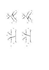
Figure 1: Diagrams for $B^{0}\to D_{s}^{+}D_{s}^{-}$ decay. The factorizable diagrams (a) and (b) contribute to $F_{a}$, and the nonfactorizable diagrams (c) and (d) do to $M_{a}$.

We consider the $B$ meson at rest for simplicity. It is convenient to use light-cone coordinates $(p^{+},p^{-},{\bf p}_{T})$, which is defined as:

$$p^{+}=\frac{p^{0}+p^{3}}{\sqrt{2}},\ \ p^{-}=\frac{p^{0}-p^{3}}{\sqrt{2}},\ \ {\bf p}_{T}=(p^{1},p^{2}).$$ (2)

Thus, expanding up to the order of $r^{2}$, we can take the $B$ meson and two $D^{(*)}$ meson momenta as:

$$P_{1}=\frac{M_{B}}{\sqrt{2}}(1,1,{\bf 0}_{T}),P_{2}=\frac{M_{B}}{\sqrt{2}}(1-r^{2},r^{2},{\bf 0}_{T}),P_{3}=\frac{M_{B}}{\sqrt{2}}(r^{2},1-r^{2},{\bf 0}_{T}),$$ (3)

where $r=M_{D^{(*)}}/M_{B}$. Putting the light (anti-)quark momenta in $B$, $D^{+}$, $D^{-}$ mesons as $k_{1}$, $k_{2}$, and $k_{3}$, respectively, we can choose

$$k_{1}=(x_{1}P_{1}^{+},0,{\bf k}_{1T}),\ \ k_{2}=(x_{2}P_{2}^{+},0,{\bf k}_{2T}),\ \ k_{3}=(0,x_{3}P_{3}^{-},{\bf k}_{3T}).$$ (4)

Unlike QCD factorization approach, we do not neglect the transverse momentum $k_{T}$ in the above expressions, by which to avoid the endpoint singularity.

If the decay involves one or two vector mesons in final states, the longitudinal polarization vectors $\epsilon_{2}^{L}$, $\epsilon_{3}^{L}$ up to the order of $r^{2}$ are given by

$$\epsilon^{L}_{2}=\frac{M_{B}}{M_{D^{*}}\sqrt{2}}(1-r^{2},-r^{2},{\bf 0}_{T}),\ \epsilon^{L}_{3}=\frac{M_{B}}{M_{D^{*}}\sqrt{2}}(-r^{2},1-r^{2},{\bf 0}_{T}),$$ (5)

and transverse polarization vectors $\epsilon_{2}^{T}$, $\epsilon_{3}^{T}$ are

$$\epsilon^{T}_{2}=(0,0,{\bf 1}_{T}),\ \ \epsilon^{T}_{3}=(0,0,{\bf 1}_{T}).$$ (6)

Then, integration over $k_{1}^{-}$, $k_{2}^{-}$, and $k_{3}^{+}$ in eq.(1) leads to:

$$\mbox{Amplitude}\sim\int\!\!dx_{1}dx_{2}dx_{3}b_{1}db_{1}b_{2}db_{2}b_{3}db_{3}\\ \mathrm{Tr}\bigl{[}C(t)\Phi_{B}(x_{1},b_{1})\Phi_{D}(x_{2},b_{2})\Phi_{D}(x_{3},b_{3})H(x_{i},b_{i},t)S_{t}(x_{i})\,e^{-S(t)}\bigr{]},$$ (7)

where $b_{i}$ is the conjugate space coordinate of the transverse momentum $k_{iT}$, and $t$ is the largest energy scale in $H$, as a function in terms of $x_{i}$ and $b_{i}$. The last term, $e^{-S(t)}$, contains two kinds of logarithms. One of the large logarithms is due to the renormalization of ultra-violet divergence $\ln tb$, the other is double logarithm $\ln^{2}b$ from the overlap of collinear and soft gluon corrections. This Sudakov form factor suppresses the soft dynamics effectively soft , so it makes a perturbative calculation of hard part $H$ applicable at the intermediate scale.

As a heavy meson, the $B$ meson wave function is not well defined, so is $D$ meson. In heavy quark limit, we may use only one independent distribution amplitude for each of them.

$$\Phi_{B}(x,b)=\frac{i}{\sqrt{6}}\left[\not\!P+M_{B}\right]\gamma_{5}\phi_{B}(x,b),$$ (8)

$$\Phi_{D}(x,b)=\frac{i}{\sqrt{6}}\gamma_{5}\left[\not\!P+M_{D}\right]\phi_{D}(x,b).$$ (9)

For the vector $D^{*}$ meson, it is expressed as:

$$\Phi_{D^{*}}(x,b)=\frac{i}{\sqrt{6}}\not\!\epsilon\left[\not\!P+M_{D^{*}}\right]\phi_{D^{*}}(x,b).$$ (10)

The hard part $H$, which is channel dependent, can be calculated perturbatively. We show the calculated formulas below for different channels.

II.1 $B^{0}\to D_{s}^{+}D_{s}^{-}$, $B^{0}_{s}\to D^{+}D^{-}$ decays

In the decay $B^{0}\to D_{s}^{+}D_{s}^{-}$, the effective Hamiltonian at scale lower than $M_{W}$ is Buchalla:1996vs :

$$H_{\mathrm{eff}}=\frac{G_{F}}{\sqrt{2}}V_{cb}^{*}V_{cd}\left[C_{1}(\mu)O_{1}(\mu)+C_{2}(\mu)O_{2}(\mu)\right],$$ (11)

$$O_{1}=(\bar{d}b)_{V-A}(\bar{c}c)_{V-A},\quad O_{2}=(\bar{c}b)_{V-A}(\bar{d}c)_{V-A}.$$ (12)

In above functions, $C_{1,2}(\mu)$ are Wilson coefficients at renormalization scale $\mu$. And summing over $\mathrm{SU}(3)_{c}$ color’s index $\alpha$, $\sum_{\alpha}\bar{q}_{\alpha}\gamma^{\nu}(1-\gamma_{5})q^{\prime}_{\alpha}$, are abbreviated to $(\bar{q}q^{\prime})_{V-A}$. Penguin operators may also have contribution, but they usually have smaller Wilson coefficients. Here we neglect these diagrams. The lowest order diagrams for the hard part $H$ calculation, are drawn in Fig.1 according to this effective Hamiltonian. Just as what we said above, there are only annihilation diagrams.

For the decay $B^{0}_{s}\to D^{+}D^{-}$, the effective Hamiltonian at scale lower than $M_{W}$ is Buchalla:1996vs :

$$H_{\mathrm{eff}}=\frac{G_{F}}{\sqrt{2}}V_{cb}^{*}V_{cs}\left[C_{1}(\mu)O_{1}^{\prime}(\mu)+C_{2}(\mu)O_{2}^{\prime}(\mu)\right],$$ (13)

$$O_{1}^{\prime}=(\bar{s}b)_{V-A}(\bar{c}c)_{V-A},\quad O_{2}^{\prime}=(\bar{c}b)_{V-A}(\bar{s}c)_{V-A}.$$ (14)

Comparing with Eqs.(11,12), the only changes in Eqs.(13,14) are the replacements of the CKM factor $V_{cd}\to V_{cs}$ and the quark $d\to s$. As we will see later the branching ratio of $B^{0}_{s}\to D^{+}D^{-}$ will be much larger than that of $B^{0}\to D_{s}^{+}D_{s}^{-}$ decay, because of this larger CKM factor $V_{cs}$. The lowest order diagrams for the hard part $H$ calculation, are then similar to $B^{0}\to D_{s}^{+}D_{s}^{-}$ decay in Fig.1 only replacing the $d$ quark by $s$ quark.

In decay $B^{0}\to D_{s}^{+}D_{s}^{-}$, we get the following analytic formulas by calculating the hard part $H$ at first order in $\alpha_{s}$. The factorizable annihilation diagrams in Fig.1a and b cancels each other, which is a result of conservation of vector current and parity invariance.

With the meson wave functions, the decay amplitude for the nonfactorizable annihilation diagrams in Fig.1(c) and (d) results in

$$M_{a}=\frac{1}{\sqrt{6}}64\pi C_{F}M_{B}^{2}\int_{0}^{1}\!\!dx_{1}dx_{2}dx_{3}\int_{0}^{\infty}\!\!b_{1}db_{1}\,b_{2}db_{2}\ \phi_{B}(x_{1},b_{1})\phi_{D_{s}}(x_{2},b_{2})\phi_{D_{s}}(x_{3},b_{2})\\ \times\Bigl{[}-x_{3}E_{m}(t_{m}^{1})h_{a}^{(1)}(x_{1},x_{2},x_{3},b_{1},b_{2})+x_{2}E_{m}(t_{m}^{2})h_{a}^{(2)}(x_{1},x_{2},x_{3},b_{1},b_{2})\Bigr{]},$$ (15)

where $C_{F}=4/3$ is the group factor of $\mathrm{SU}(3)_{c}$ gauge group. The function $E_{m}$ is defined as

$$E_{m}(t)=C_{2}(t)\alpha_{s}(t)\,e^{-S_{B}(t)-S_{D}(t)-S_{D}(t)},$$ (16)

where $S_{B}$, $S_{D}$ result from summing double logarithms caused by infrared gluon corrections and single logarithms due to the renormalization of ultra-violet divergence pqcd2 .

The functions $h_{a}^{(1)}$ and $h_{a}^{(2)}$ are the Fourier transformation of virtual quark and gluon propagators. They are defined by

$$h^{(j)}_{a}(x_{1},x_{2},x_{3},b_{1},b_{2})=$$

$$\biggl{\{}\frac{\pi i}{2}\mathrm{H}_{0}^{(1)}(M_{B}\sqrt{x_{2}x_{3}(1-2r^{2})}\,b_{1})\mathrm{J}_{0}(M_{B}\sqrt{x_{2}x_{3}(1-2r^{2})}\,b_{2})\theta(b_{1}-b_{2})$$

$$\qquad\qquad\qquad\qquad+(b_{1}\leftrightarrow b_{2})\biggr{\}}\times\left(\begin{matrix}\mathrm{K}_{0}(M_{B}F_{(j)}b_{1}),&\text{for}\quad F^{2}_{(j)}>0\\ \frac{\pi i}{2}\mathrm{H}_{0}^{(1)}(M_{B}\sqrt{|F^{2}_{(j)}|}\ b_{1}),&\text{for}\quad F^{2}_{(j)}<0\end{matrix}\right),$$ (17)

where $\mathrm{H}_{0}^{(1)}(z)=\mathrm{J}_{0}(z)+i\,\mathrm{Y}_{0}(z)$, and $F_{(j)}$s are defined by

$$F^{2}_{(1)}=x_{1}x_{3}(1-r^{2})-x_{2}x_{3}(1-2r^{2}),$$ (18)

$$F^{2}_{(2)}=x_{1}+x_{2}x_{3}+(1-r^{2})(x_{2}+x_{3}-x_{1}x_{3}-2x_{2}x_{3}).$$ (19)

The hard scale $t$’s in the amplitudes are taken as the largest energy scale in the $H$ to kill the large logarithmic radiative corrections:

$$t_{m}^{j}=\mathrm{max}(M_{B}\sqrt{|F^{2}_{(j)}|},M_{B}\sqrt{(1-2r^{2})x_{2}x_{3}},1/b_{1},1/b_{2}).$$ (20)

Applying the power counting rule established in ref.power ; dpi , we keep only the leading order contribution of $r$ expansion in the numerator of the above equation (17). The hierarchy relation $\Lambda_{QCD}\ll m_{D^{(*)}}\ll m_{B}$ is assumed. The $r^{2}$ terms are kept in the denominators of (17), since it may sometimes affect the imaginary part heavily. It is easy to see that the momentum carried by the intermediate gluon is $M_{B}\sqrt{x_{2}x_{3}(1-2r^{2})}$ which is only suppressed by a factor of $\sqrt{(1-2r^{2})}$, comparing with that of the charmless $B\to\pi\pi$ decay luy . In the heavy quark limit, $r\to 0$, the momentum of the gluon is the same for the two kinds of decays. The formulas derived here support the argument at the introduction that perturbative calculation is still applicable to the $B\to DD$ decays.

The decay width $\Gamma$ for $B^{0}\to D_{s}^{+}D_{s}^{-}$ decay is then given by

$$\Gamma(B^{0}\to D_{s}^{+}D_{s}^{-})=\frac{G_{F}^{2}M_{B}^{3}}{128\pi}(1-2r^{2})\bigl{|}V_{cb}^{*}V_{cd}M_{a}\bigr{|}^{2}.$$ (21)

Similar to decay $B^{0}\to D_{s}^{+}D_{s}^{-}$, the width for $B^{0}_{s}\to D^{+}D^{-}$ is

$$\Gamma(B^{0}_{s}\to D^{+}D^{-})=\frac{G_{F}^{2}M_{B}^{3}}{128\pi}(1-2r^{2})\bigl{|}V_{cb}^{*}V_{cs}M_{a}\bigr{|}^{2}.$$ (22)

One need only replace the $D_{s}$ wave function $\phi_{D_{s}}$ by $D$ meson. Enhanced by the CKM factor $|V_{cb}^{*}V_{cs}|^{2}$, the $B_{s}^{0}$ decay width will be larger than that of $B^{0}$ decay.

II.2 $B^{0}\to D_{s}^{*+}D_{s}^{-}$, $D_{s}^{+}D_{s}^{*-}$ and $B_{s}^{0}\to D^{*+}D^{-}$, $D^{+}D^{*-}$ decays

For final states with one pseudo-scalar and one vector mesons, only the longitudinal polarization of vector meson contribute. The decay amplitude takes the same form as the amplitude of $B$ to two pseudo-scalar mesons (15). For decay $B^{0}\to D_{s}^{*+}D_{s}^{-}$, one need only replace one of the $D_{s}$ meson distribution amplitude by $D_{s}^{*}$ one. The width of $B^{0}\to D_{s}^{+}D_{s}^{*-}$ must have the same width as $B^{0}\to D_{s}^{*+}D_{s}^{-}$. The contributions of Fig1.(a) and (b) can not be cancelled by each other because of the difference of $f_{D_{s}}$ and $f_{D_{s}^{*}}$, but it is still negligible.

Accordingly, the $B_{s}^{0}\to D^{*+}D^{-}$, $D^{+}D^{*-}$ decay amplitudes also take the same form as $B_{s}^{0}\to D^{+}D^{-}$.

II.3 $B^{0}\to D_{s}^{*+}D_{s}^{*-}$ and $B_{s}^{0}\to D^{*+}D^{*-}$ decays

There are contributions not only from the longitudinal polarization but also from two transverse polarizations in $B\to VV$ decays, where $V$ denotes the vector meson. Therefore the decays $B^{0}\to D_{s}^{*+}D_{s}^{*-}$ and $B_{s}^{0}\to D^{*+}D^{*-}$ are more complicated than $B\to PP$ or $B\to PV$.

In the covariant form, the decay amplitudes of non-factorizable annihilation diagrams are

$$M_{a}^{\prime}=\frac{1}{\sqrt{2N_{c}}}128\pi r^{2}C_{F}\int_{0}^{1}\!\!dx_{1}dx_{2}dx_{3}\int_{0}^{\infty}\!\!b_{1}db_{1}\,b_{2}db_{2}\ \phi_{B}(x_{1},b_{1})\phi_{D_{s}^{*}}(x_{2},b_{2})\phi_{D_{s}^{*}}(x_{3},b_{2})\\ \times\biggl{\{}(\epsilon_{2}\cdot\epsilon_{3})(p_{3}\cdot p_{2})(x_{2}+x_{3})\Bigl{[}E_{m}(t_{m}^{1})h_{a}^{(1)}(x_{1},x_{2},x_{3},b_{1},b_{2})-E_{m}(t_{m}^{2})h_{a}^{(2)}(x_{1},x_{2},x_{3},b_{1},b_{2})\Bigr{]}\\ +(\epsilon_{2}\cdot p_{3})(\epsilon_{3}\cdot p_{2})(x_{2}-x_{3})\Bigl{[}E_{m}(t_{m}^{1})h_{a}^{(1)}(x_{1},x_{2},x_{3},b_{1},b_{2})+E_{m}(t_{m}^{2})h_{a}^{(2)}(x_{1},x_{2},x_{3},b_{1},b_{2})\Bigr{]}\\ -i\varepsilon^{\mu\nu\rho\sigma}\epsilon_{2\mu}\epsilon_{3\nu}p_{2\rho}p_{3\sigma}(x_{2}-x_{3})\Bigl{[}E_{m}(t_{m}^{1})h_{a}^{(1)}(x_{1},x_{2},x_{3},b_{1},b_{2})-E_{m}(t_{m}^{2})h_{a}^{(2)}(x_{1},x_{2},x_{3},b_{1},b_{2})\Bigr{]}\biggr{\}},$$ (23)

with the convention $tr(\gamma_{5}\not\!a\not\!b\not\!c\not\!d)=-4i\epsilon^{\alpha\beta\gamma\rho}a_{\alpha}b_{\beta}c_{\gamma}d_{\rho}$ and $\epsilon^{0123}=1$. Just as Section (II.1), the contributions of diagrams(a) and (b) cancel each other.

If we set the $\epsilon_{i}$ to be longitudinal polarization only, the above formula goes back to the eq.(15). From the above functions, we can also see that the contributions of transverse polarizations are proportional to factors of $r^{2}$, which are suppressed comparing with longitudinal ones. In our calculation, we set $m_{c}\approx m_{D_{(s)}^{(*)}}$, just because $m_{D_{(s)}^{(*)}}-m_{c}\sim\bar{\Lambda}$. And $\Lambda/m_{D_{(s)}^{(*)}}\to 0$ in the heavy quark limit.

III Numerical Results

For $B$ meson, we use the same wave functions as other charmless $B$ decays luy ; kls , which is chosen as

$$\phi_{B}(x,b)=N_{B}x^{2}(1-x)^{2}\exp\left[-\frac{M_{B}^{2}\ x^{2}}{2\omega_{b}^{2}}-\frac{1}{2}(\omega_{b}b)^{2}\right].$$ (24)

The parameters $\omega_{b}=0.4\mbox{ GeV}$, and $N_{B}=91.745\mbox{GeV}$ which is the normalization constant using $f_{B}=190\mbox{MeV}$, are constrained by charmless B decays luy ; kls . For $B_{s}$ meson, we use the same wave function according to SU(3) symmetry. That is $\omega_{b}=0.4\mbox{ GeV}$, but $N_{B_{s}}=119.4\mbox{GeV}$, using $f_{B_{s}}=236\mbox{MeV}$.

For $D_{(s)}^{(*)}$, the distribution amplitude is taken as lu:bdsk ; dpi

$$\phi_{D_{(s)}^{(*)}}(x,b)=\frac{3}{\sqrt{2N_{c}}}f_{D_{(s)}^{(*)}}x(1-x)\{1+a_{D_{(s)}^{(*)}}(1-2x)\}.$$ (25)

Since the heavy $D_{(s)}^{(*)}$ wave function is less constrained, we use $a_{D^{(*)}}=0.6\sim 0.8\mbox{ GeV}$ and $a_{D_{s}^{(*)}}=0.2\sim 0.4\mbox{ GeV}$ to explore the sensitivity of parameters. Other parameters, such as meson mass, decay constants, the CKM matrix elements and the lifetime of $B_{(s)}$ meson pdg are given in Table 1.

Table 1: Parameters we used in numerical calculation.

	$m_{B^{0}}=5.28\mbox{GeV}$	$m_{B_{s}^{0}}=5.37\mbox{GeV}$
Mass	$m_{D^{\pm}}=1.87\mbox{GeV}$	$m_{D^{*\pm}}=2.01\mbox{GeV}$
	$m_{D_{s}^{\pm}}=1.97\mbox{GeV}$	$m_{D_{s}^{*\pm}}=2.11\mbox{GeV}$
Decay	$f_{D^{\pm}}=240\mbox{ MeV}$	$f_{D^{*\pm}}=230\mbox{MeV}$
Constants	$f_{D_{s}^{\pm}}=241\mbox{MeV}$	$f_{D_{s}^{*\pm}}=211\mbox{ MeV}$
CKM	$|V_{cd}|=0.224$	$|V_{cb}|=0.042$
	$|V_{cs}|=0.974$
Lifetime	$\tau_{B^{0}}=1.54\times 10^{-12}\mbox{ s}$	$\tau_{B_{s}^{0}}=1.46\times 10^{-12}\mbox{s}$

The calculated branching ratios in PQCD are sensitive to various parameters, such as the parameters in wave functions of $B$ and $D_{(s)}^{(*)}$. Because the wave functions are from non-perturbative effect, we can not define them exactly. In Table 2, we show examples of the sensitivity of the branching ratios to parameters in (25). The predictions of PQCD depend heavily on $\omega_{D}$ and $a_{D}$, which characterize the shape of $D_{(s)}^{(*)}$ wave function.

Table 2: The sensitivity of the decay branching ratios to change of $a_{D}$($a_{D_{s}}$).

$a_{D_{s}}$	$\mathrm{Br}(B^{0}\to D_{s}^{+}D_{s}^{-})(10^{-5})$
$0.2$	$6.2$
$0.3$	$7.8$
$0.4$	$9.8$
$a_{D}$	$\mathrm{Br}(B_{s}^{0}\to D^{+}D^{-})(10^{-3})$
$0.6$	$3.3$
$0.7$	$3.9$
$0.8$	$4.5$

From above discussion, the branching ratios within the reasonable range of parameters in wave functions are given as

$$\begin{array}[]{ll}\mathrm{Br}(B^{0}\to D_{s}^{+}D_{s}^{-})=(7.8\pm_{1.6}^{2.0})\times 10^{-5},&\mathrm{Br}(B_{s}^{0}\to D^{+}D^{-})=(3.6\pm 0.6)\times 10^{-3};\\ \mathrm{Br}(B^{0}\to D_{s}^{*+}D_{s}^{-})=(6.0\pm_{1.1}^{1.6})\times 10^{-5},&\mathrm{Br}(B_{s}^{0}\to D^{*+}D^{-})=(3.6\pm 0.6)\times 10^{-3};\\ \mathrm{Br}(B^{0}\to D_{s}^{*+}D_{s}^{*-})=(8.5\pm_{1.8}^{2.0})\times 10^{-5},&\mathrm{Br}(B_{s}^{0}\to D^{*+}D^{*-})=(6.4\pm 1.2)\times 10^{-3}.\end{array}$$ (26)

Because $f_{D_{s}^{*}}$ is smaller than $f_{D_{s}}$, we can see the branch ratio of $B^{0}\to D_{s}^{*+}D_{s}^{-}$ is a little smaller than $B^{0}\to D_{s}^{+}D_{s}^{-}$. The $\mathrm{Br}(B^{0}\to D_{s}^{*+}D_{s}^{*-})$ is larger than the others because of the extra contribution from transverse polarization.

In the decay $B\to\pi\pi$, $m_{\pi}$ is much lighter than $m_{B}$. The energy release in the decay is very large. The final $\pi$ mesons runs very fast and they may not have enough time to exchange the soft gluons and resonance. Recently, the $B\to D\pi$, $B\to D_{s}K(\phi)$ decays with one heavy $D_{(s)}^{(*)}$ meson in final state are calculated in PQCD approach lu:bdsk ; dpi . And the results are consistent with the experiments, which shows that the final state interaction may not be important in those decays, although the energy release is smaller than that in $B\to\pi\pi$ decays. Here we also calculate $B^{0}\to D_{s}^{(*)+}D_{s}^{(*)-}$ and $B_{s}^{0}\to D^{(*)+}D^{(*)-}$ decays with two heavy mesons in final states in PQCD. We get large branching ratios comparable to other predictions eeg . This may be a hint for PQCD to work good for these decays. The soft final state interaction in those decays, for example, $B^{0}\to D^{+}D^{-}$, and $D^{+}D^{-}\to D_{s}^{+}D_{s}^{-}$ through exchanging $K^{0}(\bar{K^{0}})$ is somehow smaller than the perturbative picture.

Figure 2: Contributions to the branching ratio of decay $B^{0}\to D_{s}^{+}D_{s}^{-}$ from different ranges of $\alpha_{s}/\pi$.

For consistent check, in Figure 2, we show the contribution to the branching ratio of decay $B^{0}\to D_{s}^{+}D_{s}^{-}$ from different ranges of $\alpha_{s}/\pi$, where the hard scale $t$ is given in appendix. From this figure, we find that most of contribution comes from the range $\alpha_{s}/\pi<0.3$, implying that the average scale is around $\sqrt{\Lambda_{QCD}m_{B}}$. It is then numerically confirmed that PQCD may be even applicable to $B^{0}\to D_{s}^{(*)+}D_{s}^{(*)-}$ and $B_{s}^{0}\to D^{(*)+}D^{(*)-}$ decays.

In ref.eeg , J.O. Eeg et al. computed those decays using heavy-light Chiral quark model and their results read:

$$\begin{array}[]{ll}\mathrm{Br}(B^{0}\to D_{s}^{+}D_{s}^{-})=7.0\times 10^{-5},&\mathrm{Br}(B_{s}^{0}\to D^{+}D^{-})=1.0\times 10^{-3}.\end{array}$$ (27)

Obviously, for decay $B^{0}\to D_{s}^{+}D_{s}^{-}$, we have the same result. But we got different result for decay $B_{s}^{0}\to D^{+}D^{-}$ though our results are at the same order. Unfortunately, there is no direct experimental result about these decays up to now. We hope those branching ratios will be measured soon in future and these two theories can be tested.

IV Conclusion

In this paper, we try to estimate the branching ratios of $B^{0}\to D_{s}^{(*)+}D_{s}^{(*)-}$ and $B_{s}^{0}\to D^{(*)+}D^{(*)-}$ decays in the heavy quark limit using perturbative QCD approach. These decays can occur only through annihilation diagrams because the four quarks in the final states are not the same as the ones in $B$ meson. Our numerical results agree with the heavy-light chiral quark model for $B^{0}\to D_{s}^{+}D_{s}^{-}$ and $B_{s}^{0}\to D^{+}D^{-}$ decays, which is not very small. We also give large branching ratios for channels with one or two vector mesons in final states. There is a hint for not large soft final state interactions. We hope new experimental results will give a test for our results.

References

• (1) G.P. Lepage and S. Brosky, Phys. Rev. D22, 2157 (1980); J. Botts and G. Sterman, Nucl. Phys. B225, 62 (1989).
• (2) C.-D. LΓΌ, K. Ukai and M.-Z. Yang, Phys. Rev. D63, 074009 (2001); C.-D. LΓΌ and M.Z. Yang, Eur. Phys. J. C23, 275 (2002).
• (3) Y.-Y. Keum, H.-n. Li and A. I. Sanda, Phys. Lett. B504, 6 (2001); Phys. Rev. D63, 054008 (2001).
• (4) C.-D. LΓΌ and K. Ukai, Eur. Phys. J. C28, 305 (2003); C.-D. LΓΌ, Eur. Phys. J. C24, 121 (2002); Y.Li and C.D. LΓΌ, J. Phys. G29, 2115 (2003).
• (5) H.-n. Li, Phys. Rev. D64, 014019 (2001); C.-H. Chen, Y.-Y. Keum, and H.-n. Li, Phys. Rev. D66, 054013 (2002); C.D. LΓΌ, M.-Z. Yang, Eur. Phys. J. C28, 515 (2003).
• (6) C.-H. Chen, Y.-Y. Keum, and H.-n. Li, Phys. Rev. D64, 112002 (2001).
• (7) Y.-Y. Keum, $etal.$, Phys. Rev. D69, 094018 (2004); C.D. LΓΌ, Phys. Rev. D68, 097502 (2003).
• (8) J.O.Eeg, S.Fajfer and A.Hiroth, hep-ph/0304112; hep-ph/0307042.
• (9) M. Wirbel, B. Stech, M. Bauer, Z. Phys. C29, 637 (1985); A. Ali, G. Kramer and C.-D. LΓΌ, Phys. Rev. D58, 094009 (1998).
• (10) M. Beneke, G. Buchalla, M. Neubert, C.T. Sachrajda, Phys. Rev. Lett. 83, 1914 (1999); Nucl. Phys. B591, 313 (2000).
• (11) H.-n. Li and B. Tseng, Phys. Rev. D57, 443, (1998).
• (12) G. Buchalla, A. J. Buras and M. E. Lautenbacher, Rev. Mod. Phys. 68, 1125 (1996).
• (13) Review of Particle Physics, K. Hagiwara et al., Phys. Rev. D66, 010001 (2002).