Perturbative and non-perturbative aspects of heavy–quark fragmentation

Abstract

We describe a new approach to heavy–quark fragmentation which is based on a resummed perturbative calculation and parametrization of power corrections, concentrating on the $z\longrightarrow 1$ limit, where the heavy meson carries a large fraction of the momentum of the initial quark. It is shown that the leading power corrections in this region are controlled by the scale $m(1-z)$. Renormalon analysis is then used to extend the perturbative treatment of soft and collinear radiation to the non-perturbative regime. Theoretical predictions are confronted with data on B–meson production in $e^{+}e^{-}$ annihilation.

1 Introduction

The heavy–quark fragmentation function $D(z,m^{2},\mu^{2})$ is the probability distribution to produce a heavy meson of a heavy quark. It depends on $z$, the momentum fraction of the meson, on the quark mass $m^{2}$ and on the factorization scale $\mu^{2}$. The fragmentation function has a formal definition CS as the Fourier transform

$$D(z;\mu^{2})\equiv\frac{1}{2\pi\,z}\int_{-\infty}^{\infty}\frac{dy_{-}}{y_{-}}\,\exp(i{p}y/z)\,F(py;\mu^{2}),$$ (1)

of the hadronic matrix element of a non-local operator on the light-cone ($y^{2}=0$):

$$F(py;\mu^{2})\equiv$$ (2)

$$\frac{1}{4\,N_{c}}\,\sum_{X}\,{\rm Tr}\left\{\langle 0|\mbox{$y$\raisebox{0.43057pt}{$/$}}\Psi(y)|H(p)+X\rangle\langle H(p)+X|\overline{\Psi}(0)|0\rangle_{\mu^{2}}\right\}.$$

Here the final state is composed of the measured heavy meson ($H$) carrying momentum $p$ plus anything else ($X$).

We concentrate here on inclusive observables, the prime example being the single B–meson inclusive cross section in $e^{+}e^{-}$ annihilation, shown in Fig. 1.

Figure 1: ALEPH data for the energy distribution of produced B mesons at LEP1 compared to the next–to–leading order (NLO) calculation (full line).

Cross sections of this sort can be written as a convolution

$$\frac{d\sigma(x,Q^{2})}{dx}=\int_{x}^{1}\frac{dz}{z}\,{C}(x/z,Q^{2};{\mu^{2}})\,{D}(z;{\mu^{2}})\,$$ (3)

between a process–specific coefficient function $C$, describing the hard interaction where the heavy quark is produced, and the process–independent fragmentation function $D$, defined in (1), describing the hadronization stage.

The common practice is to bridge the gap between experimental data and fixed–order calculations in QCD by means of a fragmentation model, i.e. a given functional form for ${D}(z;{\mu^{2}})$ in (3) with one or more free parameters. For heavy–quark fragmentation the most famous examples are kart ; peterson . Upon excluding the more difficult $z\longrightarrow 1$ region such fits can indeed be performed. However, the gain is limited: the relation between the parameters in these models and the matrix elements cannot be made precise. The models provides no information about the underlying hadronization dynamics. Moreover, the universality of the extracted parameters is unclear. At large $z$ fragmentation models simply fail to bridge the gap between the resummed perturbative calculation and the data. This has been recently demonstrated in a clear way Ben_haim by directly extracting the “non perturbative fragmentation component” from $e^{+}e^{-}$ data in moment space and then comparing the resulting distribution in $z$ space to models.

An important application of the heavy–quark fragmentation function which demonstrates these problems is in the description of B production in hadron colliders. The CDF collaboration found CDF an alarming discrepancy (a factor of 3) between the transverse–momentum distribution of B⁺ hadroproduction data and the standard treatment of this cross section, where a NLO calculation is convoluted with a Peterson model peterson for the fragmentation function. In the latter the free parameter was set to a standard value based on $e^{+}e^{-}$ annihilation data. Ref. CN applied a resummed perturbative calculation for the coefficient function and combined it with the relevant fragmentation effect extracted from $e^{+}e^{-}$ data in moment space, concluding that the discrepancy is much smaller. This shows that the separation between the perturbative and non-perturbative ingredients of (3) is very delicate. A naïve application of (3) simply fails: if the perturbative ingredient $C$ in (3) is taken at fixed order in $\alpha_{s}$, the required “non-perturbative” ingredient $D$ appears not to be the same in different processes.

As heavy–quark production in hadron colliders becomes increasingly important experimentally, it is evermore urgent to correctly apply perturbative QCD to such cross sections, to separate in a systematic way between the perturbative and the non-perturbative ingredients, and finally, to understand hadronization in a quantitative way. In particular, the parametrization of the fragmentation function $D$ must eventually be understood in terms of its field theoretic definition (1).

Our approach to heavy–quark fragmentation is primarily a perturbative one: we start off with a perturbative calculation of the matrix element in (2), replacing the outgoing meson by an on on-shell heavy quark, and treat non-perturbative effects, which make for the difference between the quark and the meson, as corrections. Hadronization corrections are power-suppressed: they are inversely proportional to the mass of the heavy quark $m$. The perturbative approach is appropriate so long as $m\gg\Lambda$. Thus it is definitely applicable to bottom, and probably, with some care, also to charm.

It should be kept in mind that a perturbative calculation is at all possible owing to two properties: (1) the presence of the quark mass regulating collinear divergences; and (2) the inclusive nature of the observable, which guarantees the cancellation of infrared singularities between real and virtual diagrams at any order in perturbation theory. This cancellation does leave, however, a significant trace in the expansion: Sudakov logarithms of $1-z$. This is why the ${\cal O}(\alpha_{s})$ result shown in Fig. 1 diverges at $z\longrightarrow 1$, whereas the physical cross section vanishes at this limit. It is only upon summing the $z\longrightarrow 1$ singular terms in the perturbative series to all orders (exponentiation) that the vanishing of the cross section is recovered.

2 Asymptotic Scaling

Let us first see what can be deduced on the fragmentation function from general considerations. If the quark mass $m$ is infinitely large, hadronization effects are negligible, and the fragmentation function is just $\delta(1-z)$. Taking a large but finite ratio $m/\Lambda$, one would expect the function to be somewhat smeared towards smaller $z$. This smearing is proportional to $m/\Lambda$, as expressed by the following scaling law (see e.g. Buras:qm ): $D(z)=(m/\Lambda)f((1-z)m/\Lambda)$.

This property can be formulated more precisely upon taking moments,

$$\tilde{D}(N,m^{2})\equiv\int_{0}^{1}dz\;z^{N-1}D(z,m^{2}),$$ (4)

and it can be explicitly derived CG from the field–theoretic definition (1). One can consider two limits, one where the mass becomes large and the other where the moment index $N$ gets large. For large $m$ one can match the matrix element (2) onto the heavy–quark effective theory, getting JR :

$$\frac{F(py,m^{2})}{py}\,\,\exp\left(i{p}y\right)\longrightarrow\,{{\cal F}(py\,\bar{\Lambda}/m)}+{\cal O}(\bar{\Lambda}/m),$$ (5)

namely, at the leading order in the large–$m$ expansion the dependence on $m$ and on the light–cone separation $y_{-}$ (i.e. on $py$) is coupled: the matrix element becomes a function of a single argument $py\,\bar{\Lambda}/m$. Here $\bar{\Lambda}$ is the difference between the heavy–meson mass $M$ and the heavy–quark mass $m$. For large $N$ it follows from the definition (2) and from (4) that

$$\tilde{D}(N,m^{2})\longrightarrow\left.{\frac{F(py,m^{2})}{py}\exp\left(i{p}y\right)}\right|_{py=-iN}\!\!\!\!\!\!\!+\,{\cal O}\left(\frac{1}{N}\right),$$ (6)

namely that to leading order in $1/N$ the $N$-th moment of the fragmentation function can be obtained by analytically continuing the matrix element as a function of the light–cone separation to the complex plane and evaluating it at $py=-iN$. From (5) and (6) together it follows that upon taking the simultaneous limit $m\longrightarrow\infty$ and $N\longrightarrow\infty$ with a fixed ratio $m/N$,

$$\tilde{D}(N,m^{2})\simeq\left.\,{\cal F}(py\,\bar{\Lambda}/m)\,\right|_{py=-iN}+{\cal O}\left(\frac{1}{N}\right),$$ (7)

so the fragmentation function becomes a function of a single argument $N\bar{\Lambda}/m$.

In Sec. 4 we shall see how the dependence on $m$ and $N$ through the combination $N\bar{\Lambda}/m$ follows from the large–order behaviour of the perturbative expansion in the large–$\beta_{0}$ limit. Having established Eq. (7) non-perturbatively, we know that this is indeed the leading behaviour at large $N$ and that corrections to this behaviour are suppressed by a power of $1/N$.

We see that the scale which characterizes the fragmentation process in the large $z$ region is $m(1-z)$ or, in moment space, $m/N$. This scale has a clear meaning when considering the bremsstrahlung off a heavy quark. Let us examine the emission in a frame where the quark energy $E$ is much larger than its mass. The radiation pattern (to ${\cal O}(\alpha_{s})$) is

$$\frac{dD}{dz\,d\sin^{2}\theta}\simeq\frac{C_{F}\,\alpha_{s}}{\pi}\,\frac{1}{1-z}\,\frac{\sin^{2}\theta}{(\sin^{2}\theta+m^{2}/E^{2})^{2}},$$ (8)

where only the leading term in the limit $z\longrightarrow 1$ was kept and the angle of emission $\theta$ is related to the gluon transverse momentum by $\sin^{2}\theta={k_{\perp}^{2}}/\left({E^{2}z^{2}(1-z)^{2}}\right)$. As discussed in Dokshitzer:fd , the radiation vanishes in the exact forward direction, but it peaks close to the forward direction at $\theta\,\simeq\,m/E$ (the ‘dead cone’), or in a boost-invariant formulation at $|k_{\perp}|\simeq m(1-z)$. So $m(1-z)$ is the typical transverse momentum of radiated gluons. The scaling law (7) can be understood in physical terms as the observation that the hadronization effects ($\tilde{D}(N,m^{2})$ at large $N$ and $m$) are dominated by interaction with gluons of transverse momentum $\bar{\Lambda}=M-m$.

3 Factorization

Factorization is based on the fact that dynamical processes taking place on well–separated physical scales are quantum-mechanically incoherent. This allows one to treat different subprocess independently of one another and to resum large corrections.

Eq. (3) is often regarded as the separation between perturbative and non-perturbative contributions to the cross section. However, factorization can be a much stronger tool upon considering separately the dynamics taking place on different physical scales. Consider, for example, the case of bottom production in $e^{+}e^{-}$ annihilation, shown in Fig.1. Referring to (3) one can naïvely interpret the gap between the data and some perturbative calculation as the “non-perturbative fragmentation function” and then try to bridge this gap using a model. As stressed above this interpretation leads to much confusion. Instead, the reasons for having large (perturbative and non-perturbative) corrections need to be identified and the corrections be resummed.

The first step is to separate the scales involved. Upon neglecting higher order corrections which are suppressed by powers of $m^{2}/q^{2}$ the moments of the cross section can be written as MN ; CC

$$\tilde{\sigma}(N,q^{2},m^{2})={\tilde{C}(N,q^{2};\mu_{F}^{2})}{\tilde{E}(N,\mu_{F}^{2},\mu_{0F}^{2})}\tilde{D}(N,m^{2};\mu_{0F}^{2}).$$

Choosing $\mu_{F}^{2}\sim q^{2}$ and $\mu_{0F}^{2}\sim m^{2}$, the coefficient function $\tilde{C}$ and the fragmentation function $\tilde{D}$ depend only on scales of order $q^{2}$ and $m^{2}$, respectively. The evolution factor $\tilde{E}$ can be obtained solving the Dokshitzer–Gribov–Lipatov–Altarelli–Parisi (DGLAP) equation. This factor then resums corrections depending on $\alpha_{s}\ln m^{2}/q^{2}$ to all orders. Resummation of this kind was implemented in computing the full line in Fig. 1. Clearly, this is insufficient.

Next, one observes that the subprocesses $\tilde{C}$ and $\tilde{D}$ may contain additional large corrections. One generic source of large corrections (see Beneke ) are running coupling (renormalon) effects, which induce factorial growth of the coefficient at high orders owing to the increasing sensitivity to extreme ultraviolet or infrared scales. Infrared renormalons in particular are non-summable and introduce a power–suppressed ambiguity in the perturbative definition of any quantity. Since for observable quantities this ambiguity must cancel it can serve as a probe of non–perturbative contributions.

Another source of large corrections develops at large $N$: the Sudakov logs Dokshitzer:1995ev ; CC . As stressed above the fragmentation process is dominated at large $N$ by momenta of order $m/N$. When $m$ and $m/N$ become far apart the concept of factorization applies again, and can be used to resum logs of $N$ into a Sudakov form factor. This resummation takes the form of exponentiation in moment space. A similar situation occurs in the coefficient function $\tilde{C}$, as is demonstrated in Fig. 2.

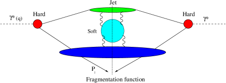
Figure 2: Factorization of bottom production in $e^{+}e^{-}$ annihilation at large $N$.

$\tilde{C}$ is dominated at large $N$ by the invariant mass $q^{2}/N$ of the unresolved jet which recoils against the measured heavy meson. The fact that this jet was also initiated by a heavy quark plays no role at this level CG : the relevant scale here is the total invariant mass of the jet. The same jet function dominates deep inelastic structure functions at large $N$ DIS ; Gardi:2002xm .

It should be emphasized that factorization (contrary to its diagrammatic proofs) is a non-perturbative concept. One should therefore expect that non-perturbative corrections on a certain scale would factorise together with the corresponding perturbative sum. In particular, this must apply to renormalon–related power corrections. In the case of Sudakov logs factorization leads to exponentiation. Going beyond the logarithmic level, one finds that power corrections on the corresponding scale exponentiate as well. This is the conceptual basis for the “shape function” approach to hadronization corrections, which has been developed in the context of event–shape distributions KS ; Korchemsky:2000kp ; Gardi:2001ny (see also DW ). This is also the basis of the approach of DIS ; Gardi:2002xm to higher twist in deep inelastic structure functions at large $N$ and of our approach CG to heavy–quark fragmentation.

4 Dressed Gluon Exponentiation

In order to deal with heavy–quark fragmentation at large $N$ both Sudakov logs and renormalons need to be taken into account. At large $N$, the perturbative coefficients are dominated by Sudakov logs. However, the resummation of the leading logarithms alone does not provide any information on power corrections. It is the subleading logs generated by the running of the coupling which produce the renormalon ambiguity Gardi:2001ny ; DGE ; CG . Their resummation is therefore essential to probe the non-perturbative regime.

From these considerations it follows that the Sudakov exponent needs to be computed to all orders rather than to some fixed logarithmic accuracy. Clearly, the full calculation cannot be done. However, relevant all–order information can be obtained from the large–$\beta_{0}$ limit corresponding to a single dressed gluon. Calculating the Sudakov exponent in this way is referred to as “Dressed Gluon Exponentiation” (DGE) Gardi:2001ny ; DGE ; CG .

A process–independent calculation of the fragmentation function (1) in the large–$\beta_{0}$ limit was performed in CG . In the light-cone axial gauge $A\cdot y=0$ where the path–ordered exponential is 1, there is just one diagram – see Fig. 3.

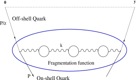
Figure 3: The diagram contributing to the fragmentation function to leading order in the flavour expansion (the large–$\beta_{0}$ limit) in the $A\cdot y=0$ gauge.

This diagram was computed using an off-shell gluon splitting function, which was derived identifying the limit where the massive quark propagator prior to the emission of the gluon is singular.

The result for the logarithmic derivative of the fragmentation function, written as a scheme invariant Borel transform, is:

$$\frac{d\tilde{D}(N,m^{2})}{d\ln m^{2}}\!=\!-\frac{C_{F}}{\beta_{0}}\int_{0}^{\infty}\!\!\!du{\left(\frac{\Lambda^{2}}{m^{2}}\right)}^{u}\!{\rm e}^{\frac{5}{3}u}\int_{0}^{1}dz\left(z^{N-1}-1\right)$$

$$\left(\frac{z}{(1-z)^{2}}\right)^{u}\left[\frac{z}{1-z}\,(1-u)+\frac{1}{2}(1-z)\,(1+u)\right],$$ (9)

where $\Lambda$ is in the ${\overline{\rm MS}}$ scheme. A generalization of this result beyond the large $\beta_{0}$ limit which fully captures the next–to–leading logarithms (NLL) was constructed in CG .

Eq. (4) takes into account the cancellation between real ($z^{N-1}$) and virtual (1) corrections. In the square brackets we distinguish between $z=1$ singular and regular terms. The former lead to logarithmically enhanced contributions in the perturbative expansion, and therefore need to be exponentiated.

According to (4) the natural scale for the renormalization of the coupling at fixed $z$ is $(1-z)^{2}m^{2}/z$. Thus, integrating over the Borel variable $u$ first is not possible for $(1-z)m\mathrel{\mathchoice{\vbox{\offinterlineskip\halign{$\m@th\displaystyle\hfil#\hfil$\cr<\crcr\sim\crcr} }}{\vbox{\offinterlineskip\halign{$\m@th\textstyle\hfil#\hfil$\cr<\crcr\sim\crcr} }}{\vbox{\offinterlineskip\halign{$\m@th\scriptstyle\hfil#\hfil$\cr<\crcr\sim\crcr} }}{\vbox{\offinterlineskip\halign{$\m@th\scriptscriptstyle\hfil#\hfil$\cr<\crcr\sim\crcr} }}}\Lambda$. As expected, perturbation theory breaks down when the gluon virtuality or its transverse momentum become comparable to the QCD scale. This constraint takes a completely different form when considered in moment space: infrared renormalons show up.

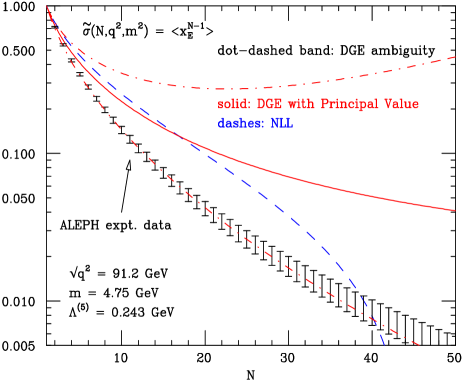
Figure 4: The perturbative DGE result compared with ALEPH data for B production in $e^{+}e^{-}$ annihilation, plotted as a function of the moment $N$.

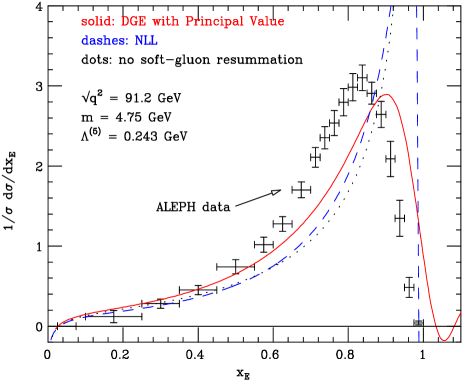
Figure 5: Same as Fig. 4, but plotted as a function of the energy fraction of the measured heavy meson.

We proceed to compute the Sudakov exponent in the large–$\beta_{0}$ limit by isolating the $z=1$ singular terms, performing the $z$-integration and then integrating over $m^{2}$. The result is:

$$\ln\tilde{D}(N,m^{2};\mu_{F0}^{2})=\frac{C_{F}}{\beta_{0}}\int_{0}^{\infty}\!\frac{du}{u}\left({\frac{{\Lambda^{2}}}{m^{2}}}\right)^{u}\times$$ (10)

$$\qquad\qquad\bigg{[}\left(\frac{m^{2}}{\mu_{F0}^{2}}\right)^{u}B_{\cal A}(u)\ln N-{B_{\tilde{D}}^{\hbox{\tiny DGE}}(u,N)}\bigg{]},$$

where

$${B_{\tilde{D}}^{\hbox{\tiny DGE}}(u,N)}=-\,{\rm e}^{\frac{5}{3}u}\,{(1-u)}\,\Gamma({-2u})\,\left({N}^{2u}-1\right).$$ (11)

The $m^{2}$ integration requires to introduce an ultraviolet subtraction: a $\mu_{F0}^{2}$–dependent counter term which cancels the $u=0$ singularity of the fragmentation function. This term is the well-known cusp anomalous dimension KR ; KM , given by $B_{\cal A}(u)\ln N$, where $B_{\cal A}(u)=1+\frac{5}{3}u+\ldots$ (we use the $\overline{\rm MS}$ factorization scheme). Note that contrary to $B_{\tilde{D}}^{\hbox{\tiny DGE}}(u,N)$ this subtraction term has just a single $\ln N$ to any order in $u$ and it is also free of infrared renormalon singularities.

According to Eq. (11), renormalons in the Sudakov exponent (10) appear at all integer and half integer $u$ values with the exception of $u=1$. It is clear from Eq. (4) that these renormalons are exclusively related to the $z\longrightarrow 1$ limit. To define the perturbative sum corresponding to $\ln\tilde{D}(N,m^{2})$ one needs to integrate over $u$ with some prescription that avoids the poles. The natural choice is the principal–value (PV) prescription (it was implemented numerically in CG ). The ambiguity in choosing a prescription is compensated by power corrections corresponding to the residues. Introducing a free parameter for each singularity one ends up with an additive correction to the perturbative Sudakov exponent having the form:

$$\ln\tilde{D}_{\hbox{\tiny NP}}({N\Lambda/m})=-\epsilon_{1}{\frac{N\Lambda}{m}}-\epsilon_{3}\left(\frac{N\Lambda}{m}\right)^{3}-\epsilon_{4}\left(\frac{N\Lambda}{m}\right)^{4}+\cdots.$$ (12)

Finally, exponentiating the result to compute $\tilde{D}(N,m^{2})$ the perturbative and non-perturbative contributions appear as two factors:

$$\tilde{D}(N,m^{2};\mu_{F0}^{2})={\tilde{D}_{\hbox{\tiny PT}}(N,m^{2};\mu_{F0}^{2})}\,\tilde{D}_{\hbox{\tiny NP}}(N\Lambda/m).$$ (13)

The leading power correction of the form $N\Lambda/{m}$ predicted in Webber_Nason is readily obtained from (12) upon expanding the exponent.

It should be stressed that in both the perturbative (10) and the non-perturbative (12) contributions to the fragmentation function we considered here only the leading terms at large $N$. At the perturbative level the result is improved CG by matching it with the full NLO coefficient. At the non-perturbative level, there may be additional ${\cal O}(\Lambda/m)$ terms which we do not parametrize, and consequently the description of the first few moments is of limited accuracy. In practice, to deal with low moments, it is useful to modify the parametrization (12) replacing $N\longrightarrow N-1$ such that the $N=1$ moment is exactly $1$, as it must be by definition.

The perturbative PV–regulated DGE result of Eq. (10), matched to the NLL and the NLO expressions and combined with the proper coefficient function, is compared as a function of $N$ with the ALEPH data in Fig. 4 (full line). In contrast with the NLL result of Ref. CC (dashed line), the DGE one does not have a Landau singularity CG and thus it extrapolates smoothly towards the values of $N\mathrel{\mathchoice{\vbox{\offinterlineskip\halign{$\m@th\displaystyle\hfil#\hfil$\cr>\crcr\sim\crcr} }}{\vbox{\offinterlineskip\halign{$\m@th\textstyle\hfil#\hfil$\cr>\crcr\sim\crcr} }}{\vbox{\offinterlineskip\halign{$\m@th\scriptstyle\hfil#\hfil$\cr>\crcr\sim\crcr} }}{\vbox{\offinterlineskip\halign{$\m@th\scriptscriptstyle\hfil#\hfil$\cr>\crcr\sim\crcr} }}}m/\Lambda$ which are beyond perturbative reach.

Also shown in Fig. 4 is the ambiguity (band shown by two dot-dashed lines) corresponding to the residue of the first renormalon pole located at $u=1/2$. The lower edge of the band just matches the data, indicating that the power correction of the form and magnitude(!) expected based on the renormalon analysis is supported by the data.

The different perturbative results are converted to $x$ space in Fig. 5. Here the significant impact of Sudakov resummation to NLL as well as that of the additional renormalon resummation achieved by DGE on the shape of the distribution is evident. Note that the shape of the DGE curve resembles that of the data but it is centered at larger $x$. Indeed, the leading effect of the non-perturbative function (assuming in (12) that only $\epsilon_{1}\neq 0$) is a shift of the entire perturbative distribution, very much the same as the leading corrections in event–shape distributions KS ; DW ; Gardi:2001ny . Finally, regarding the non-perturbative parameters $\epsilon_{n}$ as free parameters in a fit, the data can be well described. The result of a fit in moment space where the only non-perturbative correction is $\epsilon_{1}$ is shown in Fig. 6.

Figure 6: A DGE–based fit to ALEPH data. The free parameters are $\alpha_{s}$ (i.e. $\Lambda$) and the leading power correction coefficient $\epsilon_{1}$, which controls the shift of the perturbative distribution.

Upon using more non-perturbative parameters the details of the prediction (12) can be confronted with data. The analysis in CG shows that subleading non-perturbative corrections at the exponent are rather small, and the absence of a correction of the form $N^{2}\Lambda^{2}/m^{2}$ can be consistent with the data.

5 Conclusions

We described here a new approach to the QCD description of heavy–quark fragmentation concentrating on the $z\longrightarrow 1$ limit. It was first rigorously demonstrated that the non-perturbative dynamics is dominated by the scale $m(1-z)$. This scale corresponds in perturbation theory to the transverse momentum of gluons radiated from the heavy quark. Based on a renormalon analysis we extended the perturbative technique for resumming soft gluon radiation to the non-perturbative regime, identified power–like effects and separated them from the perturbative fragmentation function by means of a PV prescription. The non-perturbative contribution was then parametrized based on the renormalon ambiguity. We found that the simplest possible parametrization of power corrections which follows from renormalons, namely a shift of the perturbative distribution, is sufficient to describe the data on B production in $e^{+}e^{-}$ annihilation. This way phenomenological models for the non-perturbative fragmentation function are not needed.

The fragmentation function was treated, based on its definition (1), in a process independent way. The results are thus applicable independently of the production process, given that the corresponding coefficient function in the ${\overline{\rm MS}}$ scheme is known. Universality of the leading power corrections at large $z$ can now be tested experimentally.

References

- (1) M. Cacciari and E. Gardi, “Heavy-quark fragmentation,” Nucl. Phys. B664 (2003) 299 [hep-ph/0301047].
- (2) J. C. Collins and D. E. Soper, Nucl. Phys. B194 (1982) 445.
- (3) V.G. Kartvelishvili, A.K. Likehoded and V.A. Petrov, Phys. Lett. B78 (1978) 615.
- (4) C. Peterson, D. Schlatter, I. Schmitt and P.M. Zerwas, Phys. Rev. D27 (1983) 105.
- (5) E. Ben-Haim, P. Bambade, P. Roudeau, A. Savoy-Navarro and A. Stocchi, “Extraction of the -dependence of the non-perturbative QCD b-quark fragmentation distribution component,” [hep-ph/0302157].
- (6) D. Acosta et al. [CDF Collaboration], Phys. Rev. D65 (2002) 052005 [hep-ph/0111359].
- (7) M. Cacciari and P. Nason, Phys. Rev. Lett. 89 (2002) 122003 [hep-ph/0204025].
- (8) P. Nason, in Heavy Flavors, eds. A.J. Buras and M. Lindner, (World Scientific, Singapore, 1992) Advanced series on directions in high energy physics, vol. 10.
- (9) R. L. Jaffe and L. Randall, Nucl. Phys. B412 (1994) 79 [hep-ph/9306201].
- (10) Y. L. Dokshitzer, V. A. Khoze and S. I. Troian, J. Phys. G17 (1991) 1602.
- (11) B. Mele and P. Nason, Phys. Lett. B245 (1990) 635.
- (12) M. Cacciari and S. Catani, Nucl. Phys. B617 (2001) 253 [hep-ph/0107138].
- (13) M. Beneke, Phys. Rept. 317 (1999) 1 [hep-ph/9807443]; M. Beneke and V. M. Braun, “Renormalons and power corrections,”, in the Boris Ioffe Festschrift, At the Frontier of Particle Physics / Handbook of QCD, ed. M. Shifman (World Scientific, Singapore, 2001), vol. 3, p. 1719 [hep-ph/0010208].
- (14) Y. L. Dokshitzer, V. A. Khoze and S. I. Troian, Phys. Rev. D53 (1996) 89 [hep-ph/9506425].
- (15) E. Gardi, G. P. Korchemsky, D. A. Ross and S. Tafat, Nucl. Phys. B636 (2002) 385 [hep-ph/0203161].
- (16) E. Gardi and R. G. Roberts, Nucl. Phys. B653 (2003) 227 [hep-ph/0210429].
- (17) G. P. Korchemsky and G. Sterman, Nucl. Phys. B437 (1995) 415 [hep-ph/9411211]; in Moriond 1995: Hadronic: 0383-392, [hep-ph/9505391]; Nucl. Phys. B555 (1999) 335 [hep-ph/9902341].
- (18) G. P. Korchemsky and S. Tafat, JHEP 0010 (2000) 010 [hep-ph/0007005].
- (19) E. Gardi and J. Rathsman, Nucl. Phys. B609 (2001) 123 [hep-ph/0103217]; Nucl. Phys. B638 (2002) 243 [hep-ph/0201019].
- (20) Y. L. Dokshitzer and B. R. Webber, Phys. Lett. B404 (1997) 321 [hep-ph/9704298].
- (21) E. Gardi, Nucl. Phys. B622 (2002) 365 [hep-ph/0108222].
- (22) S. Catani, S. Dittmaier and Z. Trocsanyi, Phys. Lett. B500 (2001) 149 [hep-ph/0011222].
- (23) G. P. Korchemsky and A. V. Radyushkin, Phys. Lett. B279 (1992) 359 [hep-ph/9203222].
- (24) G. P. Korchemsky and G. Marchesini, Nucl. Phys. B406 (1993) 225 [hep-ph/9210281].
- (25) P. Nason and B. R. Webber, Phys. Lett. B395 (1997) 355 [hep-ph/9612353].