Partons and Jets at the LHC

Abstract

I review some issues related to short distance QCD and its relation to the experimental program of the Large Hadron Collider (LHC) now under construction in Geneva.

I Introduction

The tools of Quantum Chromodynamics (QCD) will be important in planning and analyzing experiments at the Large Hadron Collider (LHC). I review some of the issues here. In particular, I discuss some methods for finding new physics at the LHC in “generic” searches. Then I discuss the sources of theory error. Finally, I review the state of the art in higher order calculations that are important for confronting the experimental results with theory.

II How to find new physics at the LHC.

The most obvious way to look for new physics at the LHC is to look directly. For instance, one can look for supersymmetry by looking for the process $p+p\to{\rm squark}+{\rm antisquark}+X$, as depicted in Fig. 1.

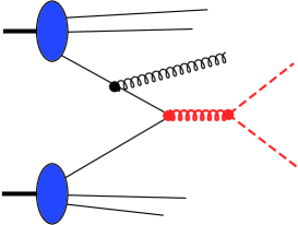
Figure 1: A diagram for $p+p\to{\rm squark}+{\rm antisquark}+X$. The squark and antisquark are created via their coupling to a gluon.

A calculation of the cross section for this process requires QCD tools QCDhandbook . One starts with the factorization formula

$${{d\sigma}}\approx\!\sum_{a,b}\int_{0}^{1}\!d\xi_{A}\int_{0}^{1}\!d\xi_{B}\ {{f_{a/A}(\xi_{A},\mu)}}\ {{f_{b/B}(\xi_{B},\mu)}}\ {{{{d\hat{\sigma}^{ab}(\mu)}}}}.$$ (1)

One needs the parton distribution functions ${{f_{a/A}(\xi,\mu)}}$ to tell the probability to find the required initial partons in the protons. We also need the hard scattering cross sections ${{{{d\hat{\sigma}^{ab}(\mu)}}}}$ for these partons to produce the squark and antisquark. This diagram illustrates a piece of the next-to-leading order (NLO) calculation of ${{{{d\hat{\sigma}^{ab}}}}}$. The emitted gluon could be included in ${{{{d\hat{\sigma}^{ab}}}}}$ or it could be included in the parton distribution functions. The calculation of ${{{{d\hat{\sigma}^{ab}}}}}$ contains a subtraction term so as not to count the gluon emission twice. Calculations are available at the NLO level for a wide variety of new physics signals of interest.

One can also use indirect methods to look for new physics at the LHC. For example, consider the Standard Model process $p+p\to W^{+}+W^{-}+X$, as depicted in Fig. 2. We still use Eq. (1) and perform a NLO calculation of the cross section for this process. If the experimental result does not agree with the theory, there must be new physics (if the discrepancy is outside the errors). Evidently, for this purpose one needs accurate calculations. Next-to-next-to-leading order would be nice (but is not available). Also, one needs a serious estimate of the errors.

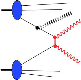
Figure 2: A diagram for $p+p\to W^{+}+W^{-}+X$.

III Jet cross sections and new physics signatures

Another indirect method to look for new physics at the LHC is to look for the cross section to make two jets, $p+p\to{\rm jet}+{\rm jet}+X$ (or, almost equivalently, one jet plus anything). Here a jet is a spray of particles. The exact definition is important, but we leave it aside for the moment. If we measure the two-jet cross section, then it is useful to measure the invariant mass of the two-jet system $M_{JJ}$. If we simply measure one jet, then a good variable to use is the so-called transverse energy $E_{T}$ of the measured jet. This is the sum of the absolute values of the transverse momenta of the particles in the jet.

To see why jet cross sections are a useful tool for looking for new physics, consider the possibility that there is some sort of new interaction at scale $\Lambda$ and that $\Lambda$ is less than the maximum value of the parton-parton c.m. energy available in the experiment (i.e. a few TeV for the LHC). One possibility is that there is a new particle with mass $M$ that decays to two jets, as depicted in Fig. 3. To see this in the one jet inclusive cross section, one would look for a threshold at $E_{T}=M/2$. Above this threshold, the cross section would be bigger than predicted in the Standard Model. To see this in the two-jet inclusive cross section, one would look for a resonance peak at $M_{JJ}=M$. That would be a spectacular signal.

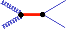
Figure 3: Production of a new particle that decays to two jets.

There are other possibilities. For instance, suppose that there is a new particle of mass $M$ that is produced in pairs. If each particle decays to two jets, one could see a threshold effect in the four-jet cross section (which, unfortunately, is known only to leading order). On the other hand, suppose that each particle decays to a lepton and a jet, as depicted in Fig. 4. In principle, this process would contribute to the one jet and two-jet inclusive cross sections. However, the signal would likely be much smaller than the background. That is because jet cross sections fall steeply with increasing $E_{T}$ because it is rare to find two incoming partons with large c.m. energy. When we look for just the jets and not the leptons, we miss seeing much of the c.m. energy in the event, so we bin the event together with events that have lower c.m. energy and thus higher cross section. The result is that to see the type of process depicted in Fig. 4, one needs to look for the leptons in addition to the jets.

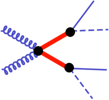
Figure 4: Production of new particles that decay to two jets and two leptons.

Now suppose that there is some sort of new interaction at scale $\Lambda$ and that $\Lambda$ is greater than the maximum value of parton-parton c.m. energy available in the experiment. Now searching for the new interaction seems hopeless. However, it is not hopeless, because the new interaction will lead to new terms in the effective lagrangian such as, for example,

$$\Delta{\cal L}={g^{\prime}\over\Lambda^{2}}\,(\bar{\psi}\psi)^{2}.$$ (2)

Here $g^{\prime}$ is a dimensionless coupling that arises from the new interactions, while $\Lambda$ is a scale parameter with dimension $m^{1}$. The factor ${1/\Lambda^{2}}$ is present for dimensional reasons: $\Delta{\cal L}$ has dimension $m^{4}$ and $(\bar{\psi}\psi)^{2}$ has dimension $m^{6}$. This term in the effective lagrangian modifies the jet cross section:

$${d\sigma_{\rm Jet}\over dE_{T}}\approx\left(d\sigma_{\rm Jet}\over dE_{T}\right)_{\!\!0}\times\left[1+({\rm const.})\,{g^{\prime}\over\alpha_{s}}\,{E_{T}^{2}\over\Lambda^{2}}\right].$$ (3)

Here the cross section with subscript 0 is the Standard Model cross section. The extra contribution depicted arises from the interference between the Standard Model amplitude and the $\Delta{\cal L}$ amplitude. There is a factor ${g^{\prime}/\Lambda^{2}}$ because that factor is present in $\Delta{\cal L}$. There is a factor $1/\alpha_{s}$ because we are replacing a Standard Model amplitude that has a factor $\alpha_{s}$. Finally, there is a factor $E_{T}^{2}$ to make the dimensions right.

Now the strategy is evident. For small $E_{T}$, the addition to the cross section is negligible. However, the addition grows with $E_{T}$. Thus we should look for a discrepancy between theory and experiment that grows with $E_{T}$.

Here is one more possibility. What if space has more than three dimensions, with the extra dimensions rolled into a little ball of size $R$? Then a quark or gluon is pointlike when viewed by a probe with wavelength $\lambda\gg R$, but not when viewed by a probe with wavelength $\lambda\lesssim R$. Then the one jet inclusive cross section should be suppressed by a form factor something like Oda

$${d\sigma_{\rm Jet}\over dE_{T}}\approx\left(d\sigma_{\rm Jet}\over dE_{T}\right)_{\!\!0}\times\exp(-RE_{T}).$$ (4)

That would be a spectacular signal.

I display in Fig. 5 the latest results CDFtalk from the CDF experiment at Fermilab on the inclusive jet cross section. These results are from Run II of the Tevatron, which is currently underway. These results extend further in $E_{T}$ than the results obtained in the previous run. The experimental measurement is compared to the prediction from next-to-leading order QCD. Theory and experiment agree within the uncertainties, indicating that “new physics” effects remain outside the range of the experiment.

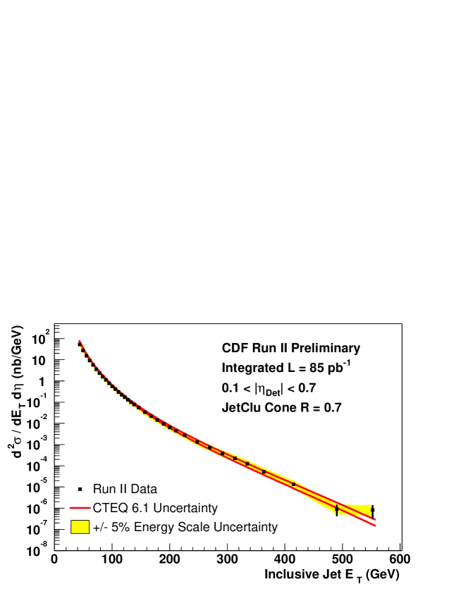
Figure 5: Preliminary Run II inclusive jet cross section from CDFCDFtalk .

One can also measure the two-jet inclusive cross section. For each event, find the two jets with the largest $E_{T}$ and use these to define the cross section

$${d\,\sigma\over d\,M_{JJ}\ d\,\eta_{JJ}\ d\,\eta^{*}}\ .$$ (5)

where $\eta_{JJ}=(\eta_{1}+\eta_{2})/2$ is the rapidity of the jet-jet c.m. system and $\eta^{*}=(\eta_{1}-\eta_{2})/2$ is the rapidity of the first jet as viewed in the jet-jet c.m. system. This is illustrated in Fig. 6. If we integrate over the rapidities to form $d\,\sigma/d\,M_{JJ}$, we get a cross section that contains essentially the same information as the one jet inclusive cross section $d\,\sigma/d\,E_{T}$, except that a resonance that decays to two jets would appear as a bump in the plot of $d\,\sigma/d\,M_{JJ}$ versus $M_{JJ}$. If, however, we look at the angular distribution $[d\sigma/d\,M_{JJ}\ d\,\eta^{*}]/[d\sigma/d\,M_{JJ}]$, we get new information. That is because vector boson exchange, which is characteristic of QCD, gives the characteristic behavior

$${d\,\sigma\over\ d\,\eta^{*}}\propto\exp(2\eta^{*})\hskip 28.45274pt\eta^{*}\gg 1\ .$$ (6)

In contrast, an s-wave distribution gives few events with $\eta^{*}>1$. More generally, a distribution with any small value of orbital angular momentum in the $s$-channel, which would be characteristic of a new physics signal, gives few events with $\eta^{*}>1$. A convenient angle variable is $\chi=\exp(2\eta^{*})$, which gives

$${d\,\sigma\over\ d\,\chi}={1\over 2\,\exp(2\eta^{*})}{d\,\sigma\over\ d\,\eta^{*}}.$$ (7)

The QCD cross section is quite flat for $\chi\gg 1$. In contrast, a new physics signal should fall off beyond $\chi\approx 3$. This method has been used for the analysis of Fermilab data. As with the one jet inclusive cross section, evidence for new physics has not been seen CDFdijet .

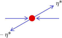
Figure 6: Two jet production as viewed in the jet-jet c.m. frame. The rapidity $\eta^{*}$ is related to the scattering angle by $\eta^{*}=-\ln\tan(\Theta^{*}/2)$.

Thus we look forward to the results at much higher $E_{T}$ or $M_{JJ}$ that will come from the LHC. In Fig. 7, I display the QCD prediction.

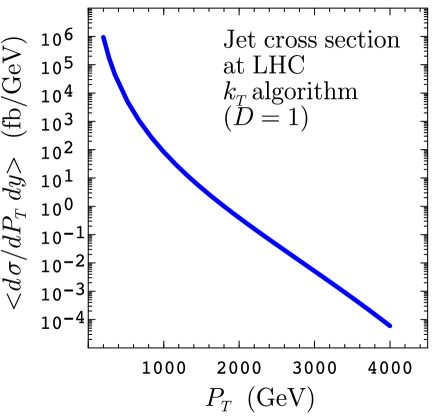
Figure 7: QCD prediction at next-to-leading order for the one jet inclusive cross section at the LHC. I plot the cross section $d\sigma/dP_{T}\,dy$ averaged over $-1<y<1$, versus $P_{T}$. The jet definition used is the successive combination jet definition, $k_{T}$ style, with joining parameter $D=1$ktjetdef . The renormalization and factorization scale are $\mu_{\rm UV}=\mu_{\rm coll}=P_{T}/2$. I use CTEQ5M parton distributions CTEQ5 . The code used is from EKSjets .

IV Theory errors

What are the errors in the theoretical prediction? Consider the example of the one jet inclusive cross section. The cross section starts with contributions of order $\alpha_{s}^{B}$ with $B=1$. We know the cross section to next-to-leading order, which means that terms of order $\alpha_{s}^{B+1}$ are also included. However, terms of order $\alpha_{s}^{B+2}$ and higher are not included. To get an estimate of the theory error arising from not including these terms, one can argue that the omitted terms are not likely to be smaller than certain order $\alpha_{s}^{B+2}$ terms that we know about. These are terms

$$\alpha_{s}^{B+2}\times[C^{(1)}_{\rm UV}\log(2\mu_{\rm UV}/E_{T})+C^{(1)}_{\rm coll}\log(2\mu_{\rm coll}/E_{T})$$

$$+C^{(2)}_{\rm UV}\log^{2}(2\mu_{\rm UV}/E_{T})+C^{(2)}_{\rm coll}\log^{2}(2\mu_{\rm coll}/E_{T})$$

$$+C^{(2)}_{\rm mixed}\log(2\mu_{\rm UV}/E_{T})\ \log(2\mu_{\rm coll}/E_{T})],$$ (8)

where $\mu_{\rm UV}$ is the renormalization scale and $\mu_{\rm coll}$ is the factorization scale. Our hypothesis is that the unknown $\alpha_{s}^{B+2}$ terms are not likely to be smaller than these terms, with the logarithms replaced by something of order 1 ($\pm\log 2$ is the conventional choice).

It is easy to estimate these terms. Consider for instance the dependence on $\mu_{\rm UV}$. The scale $\mu_{\rm UV}$ occurs in the argument of $\alpha_{s}$. We know that the derivative of the cross section with respect to $\mu_{\rm UV}$ would be zero if the cross section were calculated exactly. However the terms in Eq. (8) are absent. Thus the derivative of the calculated cross section with respect to $\mu_{\rm UV}$ is just the derivative of these terms plus higher order terms.

This leads to a simple and widely used method for estimating the theory error. We first choose a nominal “best” value of the scales, say $E_{T}/2$. Then we vary the scales by a factor of 2 about this choice. The change in the calculated cross section under this variation provides the error estimate.

Let us try this for the case of the jet cross section at the LHC. Define

$$\Delta(\mu_{\rm coll},\mu_{\rm UV})={d\sigma(\mu_{\rm UV},\mu_{\rm coll})/dE_{T}\over d\sigma(E_{T}/2,E_{T}/2)/dE_{T}}-1.$$ (9)

Then we can plot $\Delta$ versus $E_{T}$ for four choices of the scales $(\mu_{\rm UV},\mu_{\rm coll})$,

$$(E_{T}/4,E_{T}/4),(E_{T},E_{T}/4),(E_{T}/4,E_{T}),(E_{T},E_{T}).$$ (10)

The results are shown in Fig. 8. We see that the perturbative errors could reasonably be estimated at $\pm 10\%$.

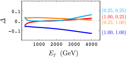
Figure 8: Variation of the jet cross section with the choice of renormalization and factorization scales. The fractional change in the cross section is shown as a function of $E_{T}$ for four different choices for $(\mu_{\rm UV},\mu_{\rm coll})$.

There is another class of theory errors. These are the errors inherent in using the factorization theorem, Eq. (1), and are of the form

$${d\sigma\over dE_{T}}=\left({d\sigma\over dE_{T}}\right)_{\rm NLO}\left\{1+{\Lambda_{1}\over E_{T}}+{\Lambda_{2}^{2}\over E_{T}^{2}}+\cdots\right\}.$$ (11)

A rough estimate is that the $\Lambda_{i}$ are of order $10\ {\rm GeV}$ for experiments at the Tevatron, with $\sqrt{s}\approx 2\ {\rm TeV}$, and perhaps somewhat larger for the LHC. This estimate arises from supposing that a jet can gain a GeV or more of $E_{T}$ from energy in the event that did not come from the hard collision, or it could loose a GeV of $E_{T}$ that falls outside of the jet cone. Then the rapid decrease of the cross section with $E_{T}$, something like $E_{T}^{-8}$ gives an estimate for $\Lambda_{1}$ of order 10.

These power suppressed terms may be important for some of the Tevatron experiments involving jets with $E_{T}<50\ {\rm GeV}$, but they are not likely to be important for jets with $E_{T}>200\ {\rm GeV}$ at the LHC.

There is one more obvious source of error in the theoretical prediction. That arises in the parton distributions that appear in Eq. (1). For momentum faction $x<0.3$, I suppose that we know the parton distributions (which are derived from experimental results) to $\pm 10\%$ or better. This would give a $\pm 20\%$ error on LHC cross sections.

For larger $x$, our knowledge of the gluon distribution is poor. To take an example, I compare the jet cross section calculated with $CTEQ5HJ$ partons with that calculated with $CTEQ5M$ partons CTEQ5 . The primary difference between these two sets lies in the large $x$ gluons. Both provide reasonable fits to the experimental data on which they are based. In Fig. 9, I plot

$$\Delta={d\sigma(CTEQ5HJ)/dE_{T}\over d\sigma(CTEQ5M)/dE_{T}}-1$$ (12)

versus $E_{T}$. We see that the difference reaches 30% for 4 TeV jets.

There has been an important development in the last couple of years: parton distribution functions now come with estimated errors CTEQ6 ; MRSTerrors . This will make the estimation of errors for the prediction of LHC cross sections more reliable.

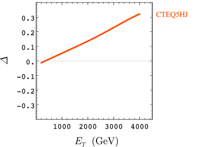
Figure 9: Jet cross section at LHC calculated with CTEQ5HJ partons compared to the cross section calculated with CTEQ5M partons CTEQ5 . The fractional difference between the calculated cross sections is plotted versus $E_{T}$.

V Reducing the perturbative theory error

It should be clear that it would be good to have more accuracy available in the theoretical predictions. To achieve this, we should try to do calculations at NNLO, i.e. including terms of order $\alpha_{s}^{B}$, $\alpha_{s}^{B+1}$, and $\alpha_{s}^{B+2}$ for a process whose theoretical expression begins at order $\alpha_{s}^{B}$.

To illustrate the point that precision is important in science, it is of interest to recall the case of $g-2$ for the muon, which was a topic of great interest last year. The ongoing experiment E821 at Brookhaven gminus2 (averaged with previous results) gives

$$(g-2)/2=11\,659\,203(8)\times 10^{-10}.$$ (13)

The corresponding calculation includes QED corrections at N⁴LO, i.e. $\alpha^{B+4}=\alpha^{5}$. The calculation also includes two loop graphs with $W$ and $Z$ bosons. There are also QCD contributions, which cannot be purely perturbative because the momentum scale is too low. One of the QCD contributions, light-by-light scattering, is illustrated in Fig. 10. This contribution had a sign error, fixed by Knecht and Nyffeler KnechtNyffeler , who found that this graph contributes $+8.3(1.2)\times 10^{-10}$. The revised theoretical contribution helps to reduce the difference between theory and experiment.

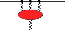
Figure 10: Light-by-light scattering, which contributes to $g-2$ of the muon.

The theory result, as summarized in Nyffeler , is

$$(g-2)/2 = 11\,659\,168(9)\times 10^{-10},$$

$$(g-2)/2 = 11\,659\,193(7)\times 10^{-10},$$ (14)

depending on whether one uses $e^{+}e^{-}$ or $\tau$ data, respectively, to obtain the contributions from vacuum polarization diagrams involving hadrons. In view of the difference between the two theory numbers, there may well be more theoretical uncertainty than indicated by the quoted errors. However, there is certainly a hint of a discrepancy between theory and experiment. This has a bearing on LHC physics because it suggests beyond the Standard Model physics of some sort at a mass scale of some fraction of a TeV. (Compare Eq. (2).) This discussion also illustrates that N^kLO calculations matter.

There are some calculations in QCD at NNLO. These important calculations are successful because they use special tricks based on calculating a simple measurable quantity. An example is the calculation Surguladze of the total cross section for $e^{+}e^{-}$ annihilation to hadrons at order $\alpha_{s}^{3}$. For more complicated quantities, such as the rapidity distribution of muon pairs produced in hadron collisionsDYatNNLO , the calculations are harder. Yet more difficult is to calculate for generic infrared safe observables. The first results for generic observables will probably come for $e^{+}e^{-}\to 3\ {\rm jets}$. In Fig. 11, we see an example of two of the graphs that must be calculated for this purpose.

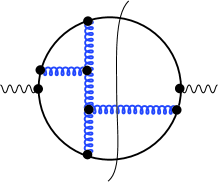
Figure 11: Two cut graphs for $e^{+}e^{-}\to 3\ {\rm jets}$ at NNLO.

In the standard analytical/numerical method for calculating such graphs, one needs an analytic result for the two loop virtual graph that appears in the left hand graph in Fig. 11. This graph is infrared divergent and is regularized by doing the calculation in $4-2\epsilon$ dimensions. (This particular graph also has an ultraviolet divergent one loop subgraph, which is treated with the aid of the same dimensional regulation.) Understandably, it is not so easy to obtain analytical results for graphs like this.

There are also cut graphs with 4 and 5 final state partons. There are infrared divergences that arise when one integrates over the phase space for these partons. Ultimately, these integrations are performed by numerical integration, but first one needs a subtraction scheme that eliminates the infrared divergences. This is also not so simple.

There has been recent progress. The analytical results for the two loop virtual graphs are available. The subtraction scheme is in progress. The progress is being made because there are several very good people working on this. For example, C. Anastasiou, M. Beneke, Z. Bern, K. G. Chetyrkin, L. Dixon, T. Gehrmann, E. W. Glover, S. Laporta, S. Moch, C. Oleari, E. Remiddi, V. A. Smirnov, J. B. Tausk, P. Uwer, O. L. Veretin, and S. Weinzierl. For a summary of this effort, see BernICHEP2002 .

I should also point out that at NLO, it is possible to do this kind of calculation by a completely numerical method beowulf . This offers evident advantages in flexibility. Perhaps a completely numerical method could help at NNLO. This avenue is, however, not being pursued at the moment.

References

- (1) R. Brock et al. [CTEQ Collaboration], Rev. Mod. Phys. 67, 157 (1995).
- (2) K. Y. Oda and N. Okada, Phys. Rev. D 66 (2002) 095005 [arXiv:hep-ph/0111298].
- (3) C. Mesropian for the CDF Collaboration, “QCD Results from the Tevatron”, talk at 8th Conference on the Intersections of Particle and Nuclear Physics (CIPANP 2003), New York, New York, 19-24 May 2003.
- (4) F. Abe et al. [CDF Collaboration], Phys. Rev. Lett. 77, 5336 (1996) [Erratum-ibid. 78, 4307 (1997)] [arXiv:hep-ex/9609011].
- (5) S. D. Ellis and D. E. Soper, Phys. Rev. D 48, 3160 (1993) [arXiv:hep-ph/9305266].
- (6) H. L. Lai et al. [CTEQ Collaboration], Eur. Phys. J. C 12, 375 (2000) [arXiv:hep-ph/9903282].
- (7) S. D. Ellis, Z. Kunszt and D. E. Soper, Phys. Rev. Lett. 69, 1496 (1992).
- (8) J. Pumplin, D. R. Stump, J. Huston, H. L. Lai, P. Nadolsky and W. K. Tung, JHEP 0207, 012 (2002) [arXiv:hep-ph/0201195].
- (9) A. D. Martin, R. G. Roberts, W. J. Stirling and R. S. Thorne, Eur. Phys. J. C 28, 455 (2003) [arXiv:hep-ph/0211080]; arXiv:hep-ph/0308087.
- (10) G. W. Bennett et al. [Muon g-2 Collaboration], Phys. Rev. Lett. 89, 101804 (2002) [Erratum-ibid. 89, 129903 (2002)] [arXiv:hep-ex/0208001].
- (11) M. Knecht and A. Nyffeler, Phys. Rev. D 65, 073034 (2002) [arXiv:hep-ph/0111058].
- (12) A. Nyffeler, arXiv:hep-ph/0305135.
- (13) L. R. Surguladze and M. A. Samuel, Phys. Rev. Lett. 66, 560 (1991) [Erratum-ibid. 66, 2416 (1991)].
- (14) C. Anastasiou, L. Dixon, K. Melnikov and F. Petriello, arXiv:hep-ph/0306192.
- (15) Z. Bern, Nucl. Phys. Proc. Suppl. 117, 260 (2003) [arXiv:hep-ph/0212406].
- (16) D. E. Soper, Phys. Rev. Lett. 81, 2638 (1998).