Neutral Higgs boson pair production via $\gamma\gamma$ collision in the minimal supersymmetric standard model at linear colliders

Abstract

We investigate in detail the $\gamma\gamma$ fusion production mechanisms of two neutral Higgs bosons ($h^{0}A^{0}$, $H^{0}A^{0}$, $h^{0}H^{0}$ and $H^{0}H^{0}$) within the framework of the mSUGRA-inspired minimal supersymmetric standard model(MSSM) at an $e^{+}e^{-}$ linear colliders, which provide a probe of the trilinear Higgs self-couplings. We calculate the dependence of the production rates on Higgs boson masses, the ratio of the vacuum expectation values $\tan\beta$ and the CMS energy $\sqrt{s}$. We find that the cross section for the $H^{0}H^{0}$ production at LC can reach $0.2~{}fb$, while the cross section of $A^{0}H^{0}$ production is only $10^{-4}\sim 10^{-3}~{}fb$ under our parameters.

PACS: 12.15.Ji, 12.60.Jv, 12.60.Fr, 14.80.Cp

I Introduction

Many efforts have been devoted to searching for Higgs bosons and the new physics beyond the standard model (SM) [1, 2], among which the minimal supersymmetric standard model (MSSM) [3] is the most promising one. Five physical Higgs bosons are predicted: one CP-odd Higgs boson ($A^{0}$), two CP-even Higgs bosons ($h^{0}$ and $H^{0}$) and two charged Higgs bosons ($H^{+}$ and $H^{-}$). Until now all those Higgs bosons haven’t been directly explored yet, only LEP2 group presents the strongest lower mass limits of $91.0~{}GeV$ and $91.9~{}GeV$ for the light CP-even and the CP-odd neutral Higgs bosons $h^{0}$ and $A^{0}$. For a top quark mass less than or equal to $174.3~{}GeV$, LEP2 group excludes the range of $0.5<\tan\beta<2.4$[4] with assuming the stop quark mixing is maximal and the conservative values for other SUSY parameters which affect the Higgs sector,

The future linear colliders will continue the work in searching for physical Higgs bosons. There are already some detailed designs of linear colliders, such as NLC[5]($\sqrt{s}=500~{}GeV$, integrated luminosity $220fb^{-1}yr^{-1}$), JLC[6]($\sqrt{s}=500GeV$, integrated luminosity $220~{}fb^{-1}yr^{-1}$), TESLA[7]($\sqrt{s}=500~{}GeV$, integrated luminosity $340~{}fb^{-1}yr^{-1}$) and CLIC[8] ($1~{}TeV<\sqrt{s}<5~{}TeV$, with a luminosity of $10^{35}~{}cm^{-2}s^{-1}$ at $\sqrt{s}=3~{}TeV$). An $e^{+}e^{-}$ LC can also be designed to operate as a $\gamma\gamma$ collider. This is achieved by using Compton backscattered photons in the scattering of intense laser photons on the initial $e^{+}e^{-}$ beams[9]. The resulting $\gamma-\gamma$ center of mass system (CMS) energy is peaked at about $0.8\sqrt{s}$ for the appropriate choices of machine parameters. In $\gamma\gamma$ collision mode at the high energy peak, we may get approximately the same luminosity as that of $e^{+}e^{-}$ collision. Therefore, a photon LC provides additional opportunities for hunting Higgs bosons.

As we know, the trilinear Higgs boson couplings can be probed in Higgs boson pair production processes. Detailed examinations of Higgs boson production and decay processes are necessary in order to detect and distinguish the signals of Higgs bosons from background. The $Z^{0}h^{0}$, $A^{0}W^{\pm}$, $H^{\pm}W^{\mp}$ associated production processes at LC were studied in Refs.[10, 11, 12, 13, 14, 15, 16], which have advantages in searching for heavy Higgs bosons. The $h^{0}A^{0}$ pair production at one-loop level via $e^{+}e^{-}$ collisions has been discussed in Ref.[17]. The neutral Higgs boson pair productions $e^{+}e^{-}\to h^{0}h^{0},H^{0}H^{0},H^{0}h^{0},A^{0}A^{0}$ and $e^{+}e^{-}\to Z^{0}h^{0}h^{0},\nu\bar{\nu}h^{0}h^{0}$ at LC were studied by A. Djouadi et al., [18, 19]. The neutral Higgs boson pair productions ($H^{0}H^{0}$, $H^{0}h^{0}$, $h^{0}h^{0}$, $A^{0}A^{0}$) at the LHC were investigated in Refs.[20, 21, 22]. The cross section for SM neutral Higgs boson pair production in $\gamma\gamma$ collision has been evaluated in Ref.[23]. The $\gamma\gamma\to h^{0}h^{0}$ and $\gamma\gamma\to A^{0}A^{0}$ pair productions in the THDM and MSSM has been calculated respectively in Ref.[24] and [25, 26]. Ref.[25] concludes that the cross section of $e^{+}e^{-}\to\gamma\gamma\to h^{0}h^{0}$ process in the framework of the MSSM at LC depends on $m_{h^{0}}$, $\tan\beta$, photon collision modes, and the mixing between stops. While in Ref.[26] it is found that for an usual mSUGRA set of parameters, $\sigma(\gamma\gamma\to A^{0}A^{0})\sim(0.1-0.2)\rm fb$ is expected.

In this paper we study the loop induced $h^{0}A^{0}$, $H^{0}A^{0}$, $h^{0}H^{0}$ and $H^{0}H^{0}$ pair productions via $\gamma\gamma$ collisions at LC in the mSUGRA-inspired MSSM. We arrange the paper as follows: In section II, we present the analytical calculation. Numerical results and discussions are given in section III. Section IV is a short summary.

II Cross Section Calculation

In our calculation we use the ’t Hooft-Feynman gauge. In the loop diagram calculation we adopt the definitions of one-loop integral functions in reference [27]. The numerical calculation of the vector and tensor loop integral functions are broken down to scalar loop integrals (Ref.[28]). The Feynman diagrams and the relevant amplitudes are generated by FeynArts package automatically [29]. The numerical calculation of the loop integrals are implemented by Mathematica package.

II.1 Calculation of the subprocess $\gamma\gamma\to\phi_{1}\phi_{2}$

We denote the subprocess under investigation as

$$\gamma(k_{1})+\gamma(k_{2})\rightarrow\phi_{1}(p_{1})+\phi_{2}(p_{2}),$$ (2.1)

where $\phi_{1}\phi_{2}$=$h^{0}A^{0}$, $H^{0}A^{0}$, $h^{0}H^{0}$ and $H^{0}H^{0}$, $k_{1}$, $k_{2}$, $p_{1}$ and $p_{2}$ are the momenta of the incoming photons and outgoing Higgs bosons. As the subprocess $\gamma\gamma\rightarrow\phi_{1}\phi_{2}$ is loop-induced at the lowest order, the one-loop order calculation can be carried out by summing all unrenormalized reducible and irreducible one-loop diagrams and the results will be finite and gauge invariant.

We give the Feynman diagrams of the $H_{i}A^{0}$ and $H_{i}H^{0}$ production processes in Fig.1 and Fig.2 respectively, where $H_{i}(i=1,2)$ represents $h^{0}$ and $H^{0}$. The possible corresponding Feynman diagrams created by exchanging the initial photons or the final Higgs bosons, are also involved in our calculation. We find that the contributions from $Z^{0}$ exchanging s-channel Feynman diagrams with fermion loops are very small because of the Furry theorem, so we do not show them in Fig.1 and remove them from our calculation. We also neglect the squark and the slepton loop diagrams in Fig.1 because of their vanishing contributions. That is because the contribution to the subprocesses $\gamma\gamma\rightarrow h^{0}A^{0},~{}H^{0}A^{0}$ from the diagram with a squark(slepton) in loop which goes clockwise cancels exactly with that which goes counterclockwise.

We denoted $\theta$ as the scattering angle between one of the photons and one of the final Higgs bosons. Then in the center of mass system we express all the four-momenta of the initial and final particles by means of the $\gamma\gamma$ CMS energy $\sqrt{\hat{s}}$ and the scattering angle $\theta$. The four-momentum components $(E,p_{x},p_{y},p_{z})$ of final particles $\phi_{1}$ and $\phi_{2}$ can be written as

$$p_{1} = \left(E_{\phi_{1}},\sqrt{E_{\phi_{1}}^{2}-m_{\phi_{1}}^{2}}\sin\theta,~{}0,~{}\sqrt{E_{\phi_{1}}^{2}-m_{\phi_{1}}^{2}}\cos\theta\right),$$

$$p_{2} = \left(E_{\phi_{2}},-\sqrt{E_{\phi_{2}}^{2}-m_{\phi_{2}}^{2}}\sin\theta,~{}0,~{}-\sqrt{E_{\phi_{2}}^{2}-m_{\phi_{2}}^{2}}\cos\theta\right),$$ (2.2)

where

$$E_{\phi_{1}}=\frac{1}{2}\left(\sqrt{\hat{s}}+(m_{\phi_{1}}^{2}-m_{\phi_{2}}^{2})/\sqrt{\hat{s}}\right),~{}~{}~{}~{}~{}E_{\phi_{2}}=\frac{1}{2}\left(\sqrt{\hat{s}}-(m_{\phi_{1}}^{2}-m_{\phi_{2}}^{2})/\sqrt{\hat{s}}\right).$$

With above expressions for the four-momenta of the final state Higgs bosons in Eq.(II.1), we can get that the three-momenta of the Higgs bosons satisfy the following relation

$$|\vec{p}_{1}|^{2}=|\vec{p}_{2}|^{2}=E_{\phi_{1}}^{2}-m_{\phi_{1}}^{2}=E_{\phi_{2}}^{2}-m_{\phi_{2}}^{2}=\frac{1}{4}\left[\hat{s}+(m_{\phi_{1}}^{2}-m_{\phi_{2}}^{2})^{2}/\hat{s}-2(m_{\phi_{1}}^{2}+m_{\phi_{2}}^{2})\right].$$

The 4-momenta of the initial photons $k_{1}$ and $k_{2}$ are

$$k_{1}=\left(\frac{1}{2}\sqrt{\hat{s}},0,0,\frac{1}{2}\sqrt{\hat{s}}\right),~{}~{}~{}~{}k_{2}=\left(\frac{1}{2}\sqrt{\hat{s}},0,0,-\frac{1}{2}\sqrt{\hat{s}}\right).$$

The Mandelstam variables are defined as

$$\begin{array}[]{lll}\hat{s}&=(k_{1}+k_{2})^{2}=(p_{1}+p_{2})^{2},\end{array}$$

$$\begin{array}[]{lll}\hat{t}&=(k_{1}-p_{1})^{2}=(k_{2}-p_{2})^{2},\end{array}$$

$$\begin{array}[]{lll}\hat{u}&=(k_{1}-p_{2})^{2}=(k_{2}-p_{1})^{2}.\end{array}$$

With the definitions above, we obtain the amplitude of the subprocess $\gamma\gamma\to\phi_{1}\phi_{2}$ with simple form. For the final states of $h^{0}A^{0}$(or $H^{0}A^{0}$), the explicit expression of the amplitude can be written as:

$${\cal M}^{H_{i}A^{0}} = \epsilon_{\mu}(k_{1})\epsilon_{\nu}(k_{2})\left\{f^{(i)}_{1}g^{\mu\nu}+f^{(i)}_{2}k_{1}^{\nu}p_{1}^{\mu}+f^{(i)}_{3}p_{1}^{\mu}p_{1}^{\nu}+f^{(i)}_{4}k_{2}^{\mu}p_{1}^{\nu}+f^{(i)}_{5}k_{2}^{\mu}p_{2}^{\nu}\right.$$ (2.3)

$$+\left.f^{(i)}_{6}k_{1}^{\nu}k_{2}^{\mu}+f^{(i)}_{7}p_{2}^{\mu}p_{2}^{\nu}+f^{(i)}_{8}k_{1}^{\nu}p_{2}^{\mu}+f^{(i)}_{9}p_{1}^{\nu}p_{2}^{\mu}+f^{(i)}_{10}p_{1}^{\mu}p_{2}^{\nu}+f^{(i)}_{11}\epsilon^{\alpha\beta\mu\nu}k_{1\alpha}k_{2\beta}\right.$$

$$+\left.f^{(i)}_{12}\epsilon^{\alpha\mu\nu\beta}k_{1\alpha}p_{1\beta}+f^{(i)}_{13}\epsilon^{\alpha\mu\nu\beta}k_{1\alpha}p_{2\beta}+f^{(i)}_{14}\epsilon^{\alpha\mu\nu\beta}k_{2\alpha}p_{1\beta}+f^{(i)}_{15}\epsilon^{\alpha\mu\nu\beta}k_{2\alpha}p_{2\beta}\right.$$

$$+\left.f^{(i)}_{16}\epsilon^{\alpha\beta\mu\sigma}k_{1\alpha}k_{2\beta}p_{1\sigma}k_{1}^{\nu}+f^{(i)}_{17}\epsilon^{\alpha\beta\mu\sigma}k_{1\alpha}k_{2\beta}p_{2\sigma}k_{1}^{\nu}\right.$$

$$+\left.f^{(i)}_{18}\epsilon^{\alpha\beta\mu\sigma}k_{1\alpha}k_{2\beta}p_{1\sigma}p_{1}^{\nu}\right\},$$

where $H_{i}$ represents $h^{0}$ or $H^{0}$, and $f^{(i)}_{j}(j=1,...,18$, $i=1$ for $h^{0}A^{0}$, $i=2$ for $H^{0}A^{0}$) are form factors. The expressions of these form factors for the two subprocesses are very similar to each other except some interaction vertices. We do not list their explicit expressions in this paper because they are very lengthy.

For the final states of $h^{0}H^{0}$ (or $H^{0}H^{0}$), the explicit expressions of the amplitudes can be written as:

$${\cal M}^{H_{k}H^{0}} = \epsilon_{\mu}(k_{1})\epsilon_{\nu}(k_{2})\left\{f^{(k)}_{1}g^{\mu\nu}+f^{(k)}_{2}k_{1}^{\nu}k_{2}^{\mu}+f^{(k)}_{3}k_{1}^{\nu}p_{1}^{\mu}+f^{(k)}_{4}k_{2}^{\mu}p_{1}^{\nu}+f^{(k)}_{5}p_{1}^{\mu}p_{1}^{\nu}+f^{(k)}_{6}k_{1}^{\nu}p_{2}^{\mu}\right.$$ (2.4)

$$+\left.f^{(k)}_{7}p_{1}^{\nu}p_{2}^{\mu}+f^{(k)}_{8}k_{2}^{\mu}p_{2}^{\nu}+f^{(k)}_{9}p_{1}^{\mu}p_{2}^{\nu}+f^{(k)}_{10}p_{2}^{\mu}p_{2}^{\nu}+f^{(k)}_{11}\epsilon^{\alpha\beta\mu\nu}k_{1\alpha}k_{2\beta}+f^{(k)}_{12}\epsilon^{\alpha\mu\nu\beta}k_{1\alpha}p_{1\beta}\right.$$

$$+\left.f^{(k)}_{13}\epsilon^{\alpha\beta\mu\nu}k_{2\alpha}p_{1\beta}+f^{(k)}_{14}\epsilon^{\alpha\beta\mu\sigma}k_{1\alpha}k_{2\beta}p_{1\sigma}k_{1}^{\nu}+f^{(k)}_{15}\epsilon^{\alpha\beta\mu\sigma}k_{1\alpha}k_{2\beta}p_{1\sigma}p_{1}^{\nu}\right\},$$

where $f^{(k)}_{j}(j=1,...15$, $k=1$ for $h^{0}H^{0}$, $k=2$ for $H^{0}H^{0}$) are form factors.

The total cross section for $\gamma\gamma\rightarrow\phi_{1}\phi_{2}$ can be expressed in the form

$$\hat{\sigma}(\hat{s})=\frac{1}{16\pi\hat{s}^{2}}\int_{\hat{t^{-}}}^{\hat{t^{+}}}d\hat{t}\overline{\sum_{spin}}|{\cal M}|^{2}$$ (2.5)

In the above equation, $\hat{t}^{\pm}=\left[(m^{2}_{\phi_{1}}+m^{2}_{\phi_{2}}-\hat{s})\pm\sqrt{(m^{2}_{\phi_{1}}+m^{2}_{\phi_{2}}-\hat{s})^{2}-4m^{2}_{\phi_{1}}m^{2}_{\phi_{2}}}~{}\right]/2$ , and the bar over summation means to take average over the initial polarizations. For the subprocess $\gamma\gamma\to H^{0}H^{0}$, an additional factor $\frac{1}{2}$ is multiplied due to the identical final particles.

II.2 Cross section of $e^{+}e^{-}\to\gamma\gamma\rightarrow\phi_{1}\phi_{2}$ process at LC

By integrating over the photon luminosity in an $e^{+}e^{-}$ linear collider, the total cross section of the process $e^{+}e^{-}\to\gamma\gamma\rightarrow\phi_{1}\phi_{2}$ can be obtained in the form

$$\sigma(s)=\int_{E_{min}/\sqrt{s}}^{x_{max}}dz\frac{d{\cal L}_{\gamma\gamma}}{dz}\hat{\sigma}(\gamma\gamma\to\phi_{1}\phi_{2}\hskip 8.53581ptat\hskip 8.53581pt\hat{s}=z^{2}s)$$ (2.6)

where $E_{min}=m_{\phi_{1}}+m_{\phi_{2}}$, and $\sqrt{s}$($\sqrt{\hat{s}}$) being the $e^{+}e^{-}$($\gamma\gamma$) CMS energy. $\frac{d\cal L_{\gamma\gamma}}{dz}$ is the distribution function of photon luminosity, which is defined as:

$$\frac{d{\cal L}_{\gamma\gamma}}{dz}=2z\int_{z^{2}/x_{max}}^{x_{max}}\frac{dx}{x}F_{\gamma/e}(x)F_{\gamma/e}(z^{2}/x)$$ (2.7)

For the initial unpolarized electrons and laser photon beams, the energy spectrum of the back scattered photon is given by [30]

$$F_{\gamma/e}=\frac{1}{D(\xi)}\left[1-x+\frac{1}{1-x}-\frac{4x}{\xi(1-x)}+\frac{4x^{2}}{\xi^{2}(1-x)^{2}}\right]$$ (2.8)

where

$$D(\xi)=(1-\frac{4}{\xi}-\frac{8}{{\xi}^{2}})\ln{(1+\xi)}+\frac{1}{2}+\frac{8}{\xi}-\frac{1}{2{(1+\xi)}^{2}},$$ (2.9)

$$\xi=\frac{4E_{0}\omega_{0}}{{m_{e}}^{2}}.$$ (2.10)

$m_{e}$ and $E_{0}$ are the mass and energy of the electron respectively, $\omega_{0}$ is the laser-photon energy, and $x$ represents the fraction of the energy of the incident electron carried by the backscattered photon. In our evaluation, we choose $\omega_{0}$ such that it maximizes the backscattered photon energy without spoiling the luminosity through $e^{+}e^{-}$ pair creation. Then we have ${\xi}=2(1+\sqrt{2})$, $x_{max}\simeq 0.83$, and $D(\xi)=1.8397$, as used in Ref.[31].

III Numerical results and discussions

III.1 Input parameters

In the following numerical evaluation, we present the results of the total cross sections of the neutral Higgs boson pair production at LC. The SM parameters are taken as : $m_{u}=66$ MeV, $m_{d}=66$ MeV, $m_{c}=1.35$ GeV, $m_{s}=0.15$ GeV, $m_{t}=174.3$ GeV, $m_{b}=4.3$ GeV, $m_{Z}=91.1876~{}GeV$, $m_{W}=80.423~{}GeV$ and $\alpha=1/127.9$[32].

We take the MSSM parameters constrained in the framework of the mSUGRA-inspired scenario as implemented in the program package SuSpect2.1[33]. In this scenario, only five sypersymmetry parameters should be input, namely $M_{0}$, $M_{1/2}$, $A_{0}$, sign of $\mu$ and $\tan\beta$, where $M_{0}$, $M_{1/2}$ and $A_{0}$ are the scalar mass at GUT scale, the universal gaugino mass and the trilinear soft breaking parameter in the superpotential terms, respectively. In the package SuSpect2.1 all the soft SUSY breaking parameters at the weak scale are obtained through Renormalization Group Equations(RGE’s) [34]. It uses 2-loop RGE’s for the gauge, Yukawa and gaugino couplings and all other RGE’s are at 1-loop order. In this work, we take $M_{1/2}$=130 GeV, $A_{0}$=200 GeV and $\mu>0$. $M_{0}$ is obtained quantitatively from the $m_{A^{0}}$(or $m_{H^{0}}$) and $\tan\beta$ values.

III.2 Discussion and analysis

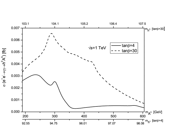
Figure 3: The cross sections $\sigma$ of the process $e^{+}e^{-}\to\gamma\gamma\to h^{0}A^{0}$, as the functions of the mass of Higgs boson $A^{0}$(starting at $m_{A^{0}}=190~{}GeV$), and $\tan\beta$ is taken as $4$ and $30$, respectively.

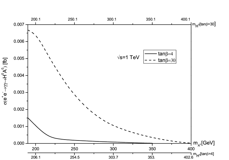
Figure 5: The cross sections $\sigma$ of the process $e^{+}e^{-}\to\gamma\gamma\to H^{0}A^{0}$, as the functions of the mass of Higgs boson $A^{0}$(starting at $m_{A^{0}}=190$ GeV), and $\tan\beta$ is taken as $4$ and $30$, respectively.

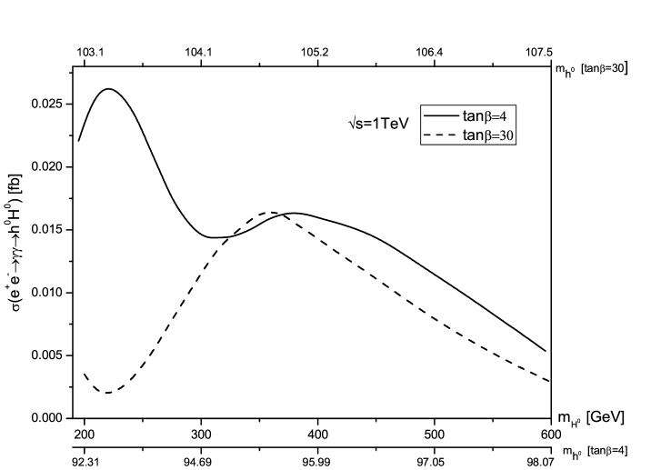
Figure 7: The cross sections $\sigma$ of the process $e^{+}e^{-}\to\gamma\gamma\to h^{0}H^{0}$, as the functions of the mass of Higgs boson $H^{0}$, and $\tan\beta$ is taken as $4$(starting at $m_{H^{0}}=195~{}GeV$) and $30$(starting at $m_{H^{0}}=200~{}GeV$), respectively.

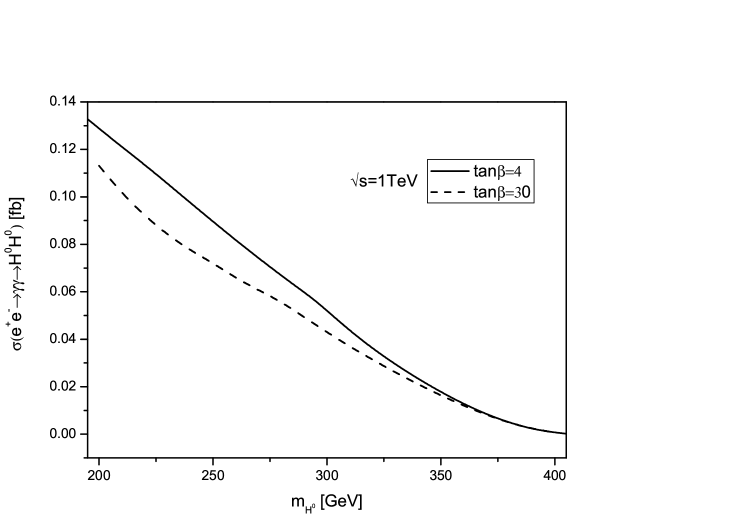
Figure 9: The cross sections $\sigma$ of the process $e^{+}e^{-}\to\gamma\gamma\to H^{0}H^{0}$, as the functions of the mass of Higgs boson $H^{0}$, and $\tan\beta$ is taken as 4(starting at $m_{H^{0}}=195$ GeV) and 30(starting at $m_{H^{0}}=200$ GeV), respectively.

We depict the curves of the production rates of the processes $e^{+}e^{-}\to\gamma\gamma\to\phi_{1}\phi_{2}$ in Fig.3-11. We note that if we take $m_{A^{0}}=200~{}GeV$(or $m_{H^{0}}=200~{}GeV$ and $300~{}GeV$) with our chosen input mSUGRA parameters($M_{1/2}=130~{}GeV$, $A_{0}=200~{}GeV$ and $\mu>0$), the mSUGRA-inspired MSSM does not permit $\tan\beta$ to be smaller than $3$ due to the experimental lower bound on the lightest Higgs boson mass $m_{h^{0}}$ in MSSM ($m_{h^{0}}>91.0~{}GeV$) [4]. Therefore, we take $\tan\beta$ varying in the range of $4\leq\tan\beta\leq 38$ with the above input parameters. For the same reason, we also exclude other parameter space regions which are inconsistent with the experimental lower bound on the $m_{h^{0}}$. That is why in Fig.3 and Fig.5 the mass of Higgs boson $A^{0}$ varies from the value of $190~{}GeV$, and the curves in Fig.7 and Fig.9 start from the Higgs boson mass $m_{H^{0}}=195~{}GeV$(for $\tan\beta=4$) and $m_{H^{0}}=200~{}GeV$(for $\tan\beta=30$) separately.

Fig.3-6 are the figures for the processes $e^{+}e^{-}\to\gamma\gamma\to h^{0}A^{0},~{}H^{0}A^{0}$ at a LC. Fig.3 displays the cross sections of the process $e^{+}e^{-}\to\gamma\gamma\to h^{0}A^{0}$ as the functions of the CP-odd Higgs boson $A^{0}$ mass (or $m_{h^{0}}$) with $\tan\beta=4$ and $30$ respectively with $e^{+}e^{-}$ colliding energy $\sqrt{s}=1~{}TeV$. The figure shows there are sophisticated structures on both two curves, which are mainly induced by the resonance effect. For example, at the vicinities of $m_{A^{0}}=m_{\chi_{2}^{+}}+m_{\chi_{1}^{+}}\sim 300~{}GeV$(for $\tan\beta=4$), $m_{A^{0}}=m_{\chi_{1}^{+}}+m_{\chi_{2}^{+}}\sim 290~{}GeV$(for $\tan\beta=30$), $m_{A^{0}}=2m_{\chi_{2}^{+}}\sim 570~{}GeV$(for $\tan\beta=4$), and $m_{A^{0}}=2m_{\chi_{2}^{+}}\sim 430~{}GeV$(for $\tan\beta=30$), we can see there are visible peaks on the two curves due to the resonance effect from loop diagrams.

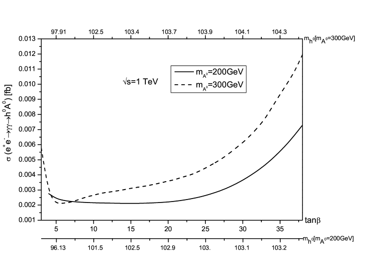
Figure 4: The cross sections $\sigma$ of the process $e^{+}e^{-}\to\gamma\gamma\to h^{0}A^{0}$, as the functions of $\tan\beta$. The mass of Higgs boson $A^{0}$ is taken as $200~{}GeV$(starting at $\tan\beta=4$) and $300~{}GeV$(starting at $\tan\beta=3$), respectively.

We plot the total cross sections of $h^{0}A^{0}$ pair productions at an $e^{+}e^{-}$ LC with $\sqrt{s}=1~{}TeV$ as the functions of $\tan\beta$ (or $m_{h^{0}}$) in Fig.4. There $A^{0}$ mass is taken to be $m_{A^{0}}=200~{}GeV$ and $300~{}GeV$ respectively. The curve for $m_{A^{0}}=200~{}GeV$ shows that in the region of $\tan\beta\leq 5$, the cross section goes down rapidly with $\tan\beta$ increasing, and then goes up with $\tan\beta$ varying from $5$ to $38$. While the curve for $m_{A^{0}}=300~{}GeV$ shows the cross section decreases in the range of $\tan\beta\leq 5$, but goes up smoothly when $\tan\beta\geq 5$. That is because the coupling strengths between Higgs boson and quark pair are related with the ratio of the vacuum expectation values.

Fig.5 displays the cross sections of the process $e^{+}e^{-}\to\gamma\gamma\to H^{0}A^{0}$ as the functions of the $A^{0}$ mass with $\tan\beta=4$ and $30$, respectively. The figure shows that the cross section decreases with the increment of the mass of the CP-odd Higgs boson $A^{0}$. We can see that the large $\tan\beta$ (i.e. $\tan\beta=30$) can enhance the cross section, while the moderate value of $\tan\beta$ may suppress the cross section.

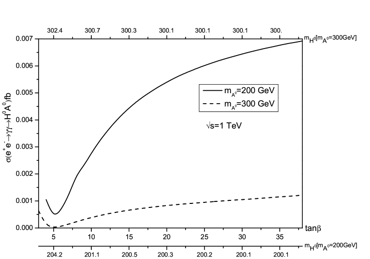
Figure 6: The cross sections $\sigma$ of the process $e^{+}e^{-}\to\gamma\gamma\to H^{0}A^{0}$, as the functions of $\tan\beta$. The mass of Higgs boson $A^{0}$ is taken as $200~{}GeV$(starting at $\tan\beta=4$) and $300~{}GeV$(starting at $\tan\beta=3$), respectively.

Fig.6 demonstrates the cross sections of the $H^{0}A^{0}$ pair production process $e^{+}e^{-}\to\gamma\gamma\to H^{0}A^{0}$ at a LC with the CMS energy $\sqrt{s}=1~{}TeV$, as the functions of $\tan\beta$ with $m_{A^{0}}=200$ and $300~{}GeV$, respectively. In the value range of $\tan\beta<5$, both curves for $m_{A^{0}}=200~{}GeV$ and $300~{}GeV$ decrease quickly, while in the range of $\tan\beta>5$ they go up with the increment of $\tan\beta$. In the region of $\tan\beta>5$, the curve for $m_{A^{0}}=200~{}GeV$ increases more quickly than that for $m_{A^{0}}=300~{}GeV$ with the increment of $\tan\beta$.

Fig.7-10 are the figures for the processes $e^{+}e^{-}\to\gamma\gamma\to h^{0}H^{0},~{}H^{0}H^{0}$ at a LC. Fig.7 shows the relationship between the cross section of the parent process $e^{+}e^{-}\to\gamma\gamma\to h^{0}H^{0}$ and $m_{H^{0}}$ with $\sqrt{s}=1~{}TeV$. The large suppression on the curve of $\tan\beta=4$ around the position of $m_{H^{0}}=m_{\chi_{1}^{+}}+m_{\chi_{2}^{+}}\sim 300GeV$, corresponds to the resonance effect. Again due to the resonance effect, the curve of $\tan\beta=30$ shows a large suppression at $m_{H^{0}}=m_{\tilde{\tau}_{1}}+m_{\tilde{\tau}_{2}}\sim 205~{}GeV$ and a large enhancement at $m_{H^{0}}=2m_{t}\sim 350~{}GeV$. We can see from the figure that the cross section with $\tan\beta=4$ is larger than the corresponding one with $\tan\beta=30$ in most of the parameter region.

In Fig.8, the curves show that the cross sections of the process $e^{+}e^{-}\to\gamma\gamma\to h^{0}H^{0}$ decrease with the increment of $\tan\beta$ in the region of $\tan\beta<10$ (for $m_{H^{0}}=200~{}GeV$) and $\tan\beta<15$ (for $m_{H^{0}}=300~{}GeV$), and then their values become to be not sensitive to $\tan\beta$.

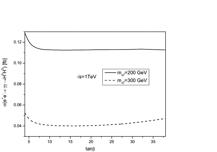
Figure 10: The cross sections $\sigma$ of the process $e^{+}e^{-}\to\gamma\gamma\to H^{0}H^{0}$, as the functions of $\tan\beta$(starting at $\tan\beta=4$). The mass of Higgs boson $H^{0}$ is taken as $200~{}GeV$ and $300~{}GeV$, respectively.

Fig.9 indicates the dependence of the cross section of $H^{0}H^{0}$ production process at LC on the mass of $H^{0}$ with $\sqrt{s}=1~{}TeV$. We find that the cross section decreases quickly with the increment of the mass of $H^{0}$. Fig.10 shows the dependence of the cross section of $e^{+}e^{-}\to\gamma\gamma\to H^{0}H^{0}$ on $\tan\beta$ with $m_{A^{0}}=200~{}GeV$ and $300~{}GeV$ respectively. Both curves show that the cross sections go down at the low $\tan\beta$ region with the increment of $\tan\beta$, and it changes smoothly in the moderate $\tan\beta$ range. When $\tan\beta>25$, the curve for $m_{A^{0}}=300~{}GeV$ goes up slowly while the curve for $m_{A^{0}}=200~{}GeV$ keeps unchanged. The cross section of $H^{0}H^{0}$ pair production at $e^{+}e^{-}$ LC is in the order of $10^{-1}$ to $10^{-2}$ in our chosen parameter space, and specially when $m_{H^{0}}=195~{}GeV$ and $\tan\beta=4$, the cross section reaches $0.13fb$.

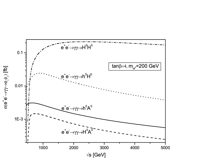
Figure 11: The cross sections $\sigma$ of the processes $e^{+}e^{-}\to\gamma\gamma\to\phi_{1}\phi_{2}$, as the functions of the $e^{+}e^{-}$ CMS energy $\sqrt{s}$.

We also plot the total cross sections of the $h^{0}A^{0}$, $H^{0}A^{0}$, $h^{0}H^{0}$ and $H^{0}H^{0}$ production processes as the functions of $\sqrt{s}$ at LC in Fig.11. There we take the input parameters $M_{1/2}=130~{}GeV$, $A_{0}=200~{}GeV$, $\mu>0$, $\tan\beta=4$ and $m_{H^{0}}=200~{}GeV$. These input parameters induce $m_{h^{0}}=92.31~{}GeV$ and $m_{A^{0}}=193.6~{}GeV$ in the mSUGRA-inspired MSSM. From this figure we find that the cross section for $H^{0}H^{0}$ production at LC is larger than the cross sections of other three channels of Higgs boson pair production processes. The cross section $\sigma(e^{+}e^{-}\to\gamma\gamma\to H^{0}H^{0})$ is of the order $10^{-2}\sim 10^{-1}$, and can exceeds $0.2~{}fb$ in some parameter space. It shows that this process could be visible at linear colliders with high enough luminosities. The curve for the cross section of $e^{+}e^{-}\to\gamma\gamma\to H^{0}A^{0}$ has the lowest value among the four curves in our chosen parameter space, which has the values in the order of $10^{-4}\sim 10^{-3}~{}fb$.

IV Summary

In this paper, We evaluate the loop induced production processes of two neutral Higgs bosons via $\gamma\gamma$ fusion, i.e. $e^{+}e^{-}\to\gamma\gamma\rightarrow\phi_{1}\phi_{2}$ ($\phi_{1}\phi_{2}=h^{0}A^{0},H^{0}A^{0},h^{0}H^{0}$ and $H^{0}H^{0}$), within the framework of the mSUGRA-inspired minimal supersymmetric standard model at $e^{+}e^{-}$ linear collider. We analyze the dependence of the total cross sections on Higgs boson masses $m_{\phi_{i}}({\phi_{i}}=H^{0},A^{0})$, the ratio of the vacuum expectation values $\tan\beta$ and colliding energy $\sqrt{s}$, respectively. With the same input parameters in Higgs sector(i.e. $\tan\beta=4$, $m_{H^{0}}=200~{}GeV$), we find that the $H^{0}H^{0}$-pair production at LC ($e^{+}e^{-}\to\gamma\gamma\to H^{0}H^{0}$) has larger production rate than the other three channels of the neutral Higgs boson pair productions in general, and can reach $0.2~{}fb$ quantitatively in our chosen parameter space, which could be visible for LC with high enough luminosity. While the cross sections of $e^{+}e^{-}\to\gamma\gamma\rightarrow h^{0}A^{0},H^{0}A^{0},h^{0}H^{0}$ at LC have smaller cross sections. The $H^{0}H^{0}$-pair production has the lowest production rate among all the four channels in our chosen parameter space, which has the values of the order $10^{-4}\sim 10^{-3}~{}fb$.

Acknowledgments: This work was supported in part by the National Natural Science Foundation of China and a grant from the University of Science and Technology of China.

Figure 1: The Feynman diagrams of the subprocess $\gamma\gamma\to H_{i}A^{0}$, where $H_{i}$ denotes $h^{0}$ and $H^{0}$, $f$ can be quark, lepton or chargino, and $\tilde{f}$ is squark or slepton. The meaning of other notations in the figures are as follows: (a): $s_{1}s_{2}s_{3}s_{4}$=$G^{-}G^{-}G^{-}H^{-}$,$G^{-}G^{-}W^{-}H^{-}$, $W^{-}G^{-}G^{-}H^{-}$, $W^{-}G^{-}W^{-}H^{-}$, $G^{-}W^{-}G^{-}H^{-}$, $G^{-}W^{-}W^{-}H^{-}$, $W^{-}W^{-}G^{-}H^{-}$, $W^{-}W^{-}W^{-}H^{-}$, $H^{-}H^{-}H^{-}G^{-}$, $H^{-}H^{-}H^{-}W^{-}$; (b):$s_{1}s_{2}s_{3}s_{4}$=$G^{-}H^{-}H^{-}G^{-}$, $G^{-}H^{-}H^{-}W^{-}$, $W^{-}H^{-}H^{-}G^{-}$, $W^{-}H^{-}H^{-}W^{-}$, $H^{-}G^{-}G^{-}H^{-}$, $H^{-}G^{-}W^{-}H^{-}$, $H^{-}W^{-}G^{-}H^{-}$, $H^{-}W^{-}W^{-}H^{-}$; (d):when the propagator is $G^{0}$, $s_{1}s_{2}s_{3}$=$u_{\pm}u_{\pm}u_{\pm}$, $G^{-}G^{-}W^{-}$, $W^{-}W^{-}G^{-}$, and when the propagator is $Z^{0}$, $s_{1}s_{2}s_{3}$=$u_{\pm}u_{\pm}u_{\pm}$, $H^{-}H^{-}H^{-}$, $G^{-}G^{-}G^{-}$, $W^{-}W^{-}W^{-}$, $G^{-}G^{-}W^{-}$, $G^{-}W^{-}G^{-}$,$W^{-}G^{-}W^{-}$,$W^{-}W^{-}G^{-}$; (e): $s_{1}s_{2}s_{3}$=$W^{-}G^{-}H^{-}$, $H^{-}H^{-}W^{-}$, $W^{-}W^{-}H^{-}$; (f): $s_{1}s_{2}s_{3}$=$H^{-}H^{-}G^{-}$, $G^{-}G^{-}H^{-}$, $W^{-}W^{-}H^{-}$, $H^{-}H^{-}W^{-}$.

Figure 2: The Feynman diagrams of the subprocess $\gamma\gamma\to$ $H_{i}H^{0}$, where $H_{i}$ denotes $h^{0}$ and $H^{0}$, $f$ can be quark, lepton or chargino, $\tilde{f}$ is squark or slepton, and $u$ denotes $u_{+}$ or $u_{-}$(the ghost field of $W$ boson). The figures form (a) to (j) are for both the $h^{0}H^{0}$ and $H^{0}H^{0}$ production processes, while (k) and (m) are for the $H^{0}H^{0}$ final states only. $s_{i}$($i=1,...4$) can be $H^{-}$,$G^{-}$ or $W^{-}$, and they appear in the figures in the following way: (a):there are two cases permitted: (i)$s_{1}=s_{2}=s_{3}$; (ii) $s_{1}s_{2}s_{3}=$$G^{-}W^{-}G^{-}$, $G^{-}W^{-}W^{-}$, $G^{-}G^{-}W^{-}$, $W^{-}W^{-}G^{-}$, $W^{-}G^{-}G^{-}$, $W^{-}G^{-}W^{-}$. (b):there are five cases permitted: $s_{1}=s_{2}=s_{3}=s_{4}$; (ii)$s_{1}=s_{2}\neq s_{3}=s_{4}$; (iii)$s_{1}=s_{4}$, and $s_{2}s_{3}=$$G^{-}W^{-}$ or $W^{-}G^{-}$, (iv)$s_{2}=s_{3}$, and $s_{1}s_{4}=$$G^{-}W^{-}$ or $W^{-}G^{-}$. (v)$s_{1}s_{4}=$$G^{-}W^{-}$ or $W^{-}G^{-}$, and $s_{2}s_{3}=$$G^{-}W^{-}$ or $W^{-}G^{-}$. (c):$s_{1}s_{2}s_{3}=$, $H^{-}H^{-}H^{-}$, $G^{-}G^{-}G^{-}$, $W^{-}W^{-}W^{-}$, $G^{-}G^{-}W^{-}$, $G^{-}W^{-}G^{-}$, $W^{-}G^{-}W^{-}$, $G^{-}W^{-}W^{-}$. (d): $s_{1}s_{2}s_{3}=$$H^{-}H^{-}W^{-}$, $G^{-}G^{-}W^{-}$, $W^{-}G^{-}H^{-}$, $W^{-}G^{-}G^{-}$, $G^{-}W^{-}W^{-}$, $W^{-}W^{-}H^{-}$, $W^{-}W^{-}G^{-}$. (i): $s_{1}s_{2}s_{3}=$ $H^{-}H^{-}H^{-}$, $G^{-}G^{-}G^{-}$, $G^{-}W^{-}G^{-}$.

Figure 8: The cross sections $\sigma$ of the process $e^{+}e^{-}\to\gamma\gamma\to h^{0}H^{0}$, as the functions of $\tan\beta$(starting at $\tan\beta=4$). The mass of Higgs boson $A^{0}$ is taken as $200~{}GeV$ and $300~{}GeV$, respectively.

References

- [1] S.L. Glashow, Nucl. Phys. 22(1961)579; S. Weinberg, Phys. Rev. Lett. 1(1967)1264; A. Salam, Proc. 8th Nobel Symposium Stockholm 1968, ed. N. Svartholm (Almquist and Wiksells, Stockholm 1968) p.367; H.D. Politzer, Phys. Rep. 14(1974)129.
- [2] P.W. Higgs, Phys. Lett. 12(1964)132, Phys. Rev. Lett. 13 (1964)508; Phys. Rev. 145(1966)1156; F.Englert and R. Brout, Phys. Rev. Lett. 13(1964)321; G.S. Guralnik, C.R. Hagen and T.W.B. Kibble, Phys. Rev. Lett. 13(1964)585; T.W.B. Kibble, Phys. Rev. 155(1967)1554.
- [3] H. E. Haber and G. L. Kane, Phys. Rep. 117 (1985) 75.
- [4] ‘Searches for the Neutral Higgs Bosons of the MSSM: Preliminary Combined Results Using LEP Data Collected at Energies up to 209 GeV’, Aleph, Delphi, L3 and OPAL Collaborations, The LEP working group, LHWG Note 2002-04, Submitted to EPS‘01 in Budapest and Lepton-Photon ’01 in Rome, hep-ex/0107030.
- [5] C. Adolphsen et al. (International Study Group Collaboration), “International study group progress report on linear collider development,” SLAC-R-559 and KEK-REPORT-2000-7 (April, 2000).
- [6] N. Akasaka et al., “JLC design study,” KEK-REPORT-97-1
- [7] R. Brinkmann, K. Flottmann, J. Rossbach, P. Schmuser, N. Walker and H. Weise(editor), “TESLA: The superconducting electron positron linear collider with an integrated X-ray laser laboratory. Technical design report, Part 2: The Accelerator,” DESY-01-11 (March, 2001).
- [8] “A 3TeV Linear Collider Based on CLIC Technology”, G.Guignard(editor), CERN-2000-008.
- [9] I.F. Ginzburg, G.L. Kotkin, V.G. Serbo and V.I. Telov, Nucl. Instrum. Meth. Nucl. Instrum. Meth. A205, 47(1983); I.F. Ginzburg, G.L. Kotkin, V.G. Panfil, V.G. Serbo and V.I. Telov, Nucl. Instrum. Meth. A219, 5(1984);
- [10] G.J.Gounaris,P.I. Porfyriadis and F.M.Renard, Eur.Phys.J. C20(2001)659-675, hep-ph/0103135.
- [11] Yin Jun, Ma Wen-Gan, Zhang Ren-You and Hou Hong-Sheng, Phys. Rev. D66(2002)095008.
- [12] A. Arhrib, M.C. Peyranere, W. Hollik and G. Moultaka, Nucl. Phys. B581 (2000) 34.
- [13] S. Kanemura, Eur. Phys. J. C17 (2000) 473.
- [14] S.H. Zhu, hep-ph/9901221.
- [15] Heather E. Logan, Shufang Su, Phys.Rev. D66 (2002) 035001, hep-ph/0203270.
- [16] Zhou Fei, Ma Wen-Gan, Jiang Yi, Li Xue-Qian and Wan Lang-Hui, Phys. Rev. D64 (2001) 055005.
- [17] Volker Driesen and Wolfgang Hollik, Z.Phys. C68 (1995) 485-490, hep-ph/9504335.
- [18] A. Djouadi, V. Driesen and C. Junger, Phys. Rev. D54 (1996)759
- [19] A. Djouadi, W. Kilian, M. Muhlleitner, P.M. Zerwas, Eur.Phys.J.C10:27-43,1999.
- [20] A.A. Barrientos Bendezu and B.A. Kniehl, Phys. Rev. D64 (2001) 035006.
- [21] A.Belyaev,M.Drees, O.J.P.Eboli, J.K.Mizuhoshi and S.F.Novaes, CERN-TH/99-325, hep-ph/9910400.
- [22] A. Djouadi, W. Kilian, M. Muhlleitner, P.M. Zerwas, Eur.Phys.J.C10:45-49,1999.
- [23] G.V.Jikia, Nucl. Phys. B412(1994)57
- [24] Sun La-Zhen, Liu Yao-Yang, Phys.Rev.D54(1996)3563
- [25] Shou Hua Zhu, Chong Sheng Li and Chong Shou Gao, Phys.Rev. D58 (1998) 015006, hep-ph/9710424.
- [26] G.J.Gounaris,P.I. Porfyriadis, Nucl.Phys. B592 (2001)203-218, hep-ph/0007110;
- [27] Bernd A. Kniehl, Phys. Rep. 240(1994)211.
- [28] G. Passarino and M. Veltman, Nucl. Phys. B160, 151(1979).
- [29] J. Küblbeck, M. Böhm and A. Denner, Comput. Phys. Commun. 60 (1990) 165; T. Hahn, KA-TP-5-1999, hep-ph/9905354.
- [30] V. Telnov, Nucl. Instrum. Methods Phys. Res. A294(1990)72; L. Ginzburg, G. Kotkin and H. Spiesbergerm, Fortschr. Phys. 34(1986)687.
- [31] K. Cheung, Phys.Rev. D47(1993)3750.
- [32] K.Hagiwara et al, Phys.ReV.D66(2002)1.
- [33] Abdelhak Djouadi, Jean-Loic Kneur and Gilbert Moultaka, PM-02-39 and CERN TH/2002-32.
- [34] V. Barger, M.S. Berger and P. Ohmann, Phys. Rev. D47 (1993) 1093, D47 (1993) 2038; V. Barger, M.S. Berger, P. Ohmann and R.J. N. Phillips, Phys. Lett. B314 (1993) 351; V. Barger, M.S. Berger and P. Ohmann, Phys. Rev. D49 (1994) 4908.