Abstract

We study the process $gg\to b\bar{b}H^{+}H^{-}$ at large $\tan\beta$, where it represents the dominant production mode of charged Higgs boson pairs in a Type II 2-Higgs Doublet Model, including the Minimal Supersymmetric Standard Model. The ability to select this signal would in principle enable the measurements of some triple-Higgs couplings, which in turn would help understanding the structure of the extended Higgs sector. We outline a selection procedure that should aid in disentangling the Higgs signal from the main irreducible background. This exploits a signature made up by ‘four $b$-quark jets, two light-quark jets, a $\tau$-lepton and missing energy’. While, for $\tan\beta\>\raisebox{-1.93748pt}{$\stackrel{{\scriptstyle\textstyle>}}{{\sim}}$}\>30$ and over a significant $M_{H^{\pm}}$ range above the top mass, a small signal emerges already at the Large Hadron Collider after 100 fb^-1, ten times as much luminosity would be needed to perform accurate measurements of Higgs parameters in the above final state, rendering this channel a primary candidate to benefit from the so-called ‘Super’ Large Hadron Collider option, for which a tenfold increase in instantaneous luminosity is currently being considered.

Keywords:
Beyond Standard Model, Two Higgs Doublet Models, Supersymmetry, Charged Higgs Bosons.

1 Introduction

Charged Higgs bosons appear in the particle spectrum of a general 2-Higgs Doublet Model (2HDM). We are concerned here with the case of a Type II 2HDM [1], possibly in presence of minimal Supersymmetry (SUSY), the combination of the two yielding the so-called Minimal Supersymmetric Standard Model (MSSM). To stay with the Higgs sector of the extended model, unless two or more neutral Higgs states are detected at the Large Hadron Collider (LHC), only the discovery of a spinless charged Higgs state would unquestionably confirm the existence of new physics beyond the Standard Model (SM), since such a field has no SM counterpart. In the MSSM, e.g., if $M_{H^{\pm}},M_{A^{0}},M_{H^{0}}\gg M_{h^{0}}$ and $\tan\beta$ is below 10 or so, the only available Higgs state ($h^{0}$) is indistinguishable from the one of the SM: this is the so-called ‘decoupling scenario’.

Not surprisingly then, a lot of effort has been put lately, by theorists and experimentalists alike, in clarifying the Higgs discovery potential of the LHC in the charged Higgs sector [2]. (This is particularly true within the MSSM scenario, where one could also exploit interactions between the Higgs and sparticle sectors [3] in order to extend the reach of charged Higgs bosons at the LHC, beyond the standard channels.) Results are now rather encouraging, as charged Higgs bosons could indeed provide the key to unveil the nature of EWSB over a large area in $M_{H^{\pm}}$ and $\tan\beta$, as they may well be the next available Higgs boson states, other than the $h^{0}$, provided $\tan\beta$ is rather large (above 10 or so). Once the $H^{\pm}$ and $h^{0}$ Higgs bosons will have been detected, the next step would be to determine their interactions with SM particles, among themselves and also with the other two neutral Higgs states, $H^{0}$ and $A^{0}$. While the measurement of the former would have little to teach us as whether one is in presence of a general Type II 2HDM or indeed the MSSM, constraints on the latter two would certainly help to clarify the situation in this respect. In fact, triple-Higgs vertices enter directly the functional form of the extended Higgs potential and, once folded within a suitable Higgs production process, may lead to the measurement of fundamental terms of the extended model Lagrangian. As the $H^{\pm}$ states have a finite Electro-Magnetic (EM) charge, the first Lagrangian term of relevance would be the one involving two such states and a neutral Higgs boson: chiefly, the vertices $H^{+}H^{-}\Phi^{0}$, where $\Phi^{0}=h^{0}$ and $H^{0}$. This requires the investigation of hard scattering processes with two charged Higgs bosons in the final state, as their direct couplings to valence quarks in the proton would be very small, hence inhibiting processes like: e.g., $q\bar{q}^{\prime}\to H^{\pm*}\to H^{\pm}\Phi^{0}$.

2 Hadroproduction of charged Higgs boson pairs

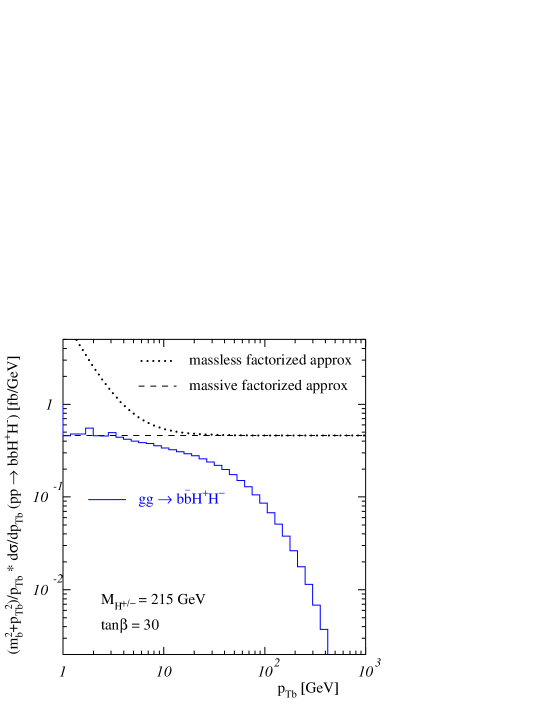
Figure 2: Transverse momentum distribution (multiplied by $((p^{T}_{b})^{2}+m_{b}^{2})/p^{T}_{b}$) of $b$-quarks ($m_{b}=$4.25 GeV) in $gg\to b\bar{b}H^{+}H^{-}$ compared to factorised expectations for massless and massive partons.

A summary of all possible production modes of charged Higgs boson pairs at the LHC in the MSSM can be found in Ref. [4]. Three channels dominate $H^{+}H^{-}$ phenomenology at the LHC: (i) $q\bar{q}\to H^{+}H^{-}$ (via intermediate $\gamma^{*}/Z^{0*}$ production but also via Higgs-strahlung off incoming $b\bar{b}$ pairs) [5]; (ii) $gg\to H^{+}H^{-}$ (primarily via a loop of top and bottom (s)quarks) [6]; (iii) $qq\to qqH^{+}H^{-}$ (via vector boson fusion) [4]. Corresponding cross sections are found in Fig. 2 of Ref. [4]. For all phenomenologically relevant $\tan\beta$ values it is essentially the first process which dominates. One important aspect should be noted here though, concerning the simulation of the $b\bar{b}$ component of the $q\bar{q}\to H^{+}H^{-}$ process, which can become the dominant contribution to the cross section of process (i) at very large $\tan\beta$ values. In fact, the use of a ‘phenomenological’ $b$-quark parton density, as available in most Parton Distribution Function (PDF) sets currently on the market, requires crude approximations of the partonic kinematics, which result in a mis-estimation of the corresponding contribution to the total production cross section. (The problem is well known already from the study of the leading production processes of charged Higgs bosons at the LHC, namely, $\bar{b}g\rightarrow\bar{t}H^{+}$ and $gg\to b\bar{t}H^{+}$: see, e.g., [8, 10].) In practice, the $b$-(anti)quark in the initial state comes from a gluon in the proton beam splitting into a collinear $b\bar{b}$-pair, resulting in large factors of $\sim\alpha_{\rm S}\log(\mu_{F}/m_{b})$, where $\mu_{F}$ is the factorisation scale. These terms are then re-summed to all orders, $\sum_{n}\alpha_{\rm S}^{n}\log^{n}(\mu_{F}/m_{b})$, in evaluating the phenomenological $b$-quark PDF. In contrast, in using a gluon density while computing the ‘twin’ process (iv) $gg\to b\bar{b}H^{+}H^{-}$ (see Fig. 1 for the associated Feynman graphs), one basically only includes the first terms ($n=1$) of the corresponding two series, when the $b$ and $\bar{b}$ in the final state are produced collinearly to the incoming gluon directions. It turns out that, for $\mu_{F}\gg m_{b}$, as it is the case here if one uses the standard choice of factorisation scale $\mu_{F}\>\raisebox{-2.15277pt}{$\stackrel{{\scriptstyle\textstyle>}}{{\sim}}$}\>2M_{H^{\pm}}$, the re-summed terms are large and over-compensate the contribution of the large transverse momentum region available in the gluon-induced case. In the end, differences between the two cross sections as large as one order of magnitude are found, well in line with the findings of Refs. [8] and [10], if one considers that two $g\to b\bar{b}$ splittings are involved here.

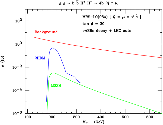
Figure 5: Total cross sections as a function of $M_{H^{\pm}}$ for processes (1) (with finite width effects) and (2) yielding the signature (5), including all decay BRs and after the kinematic cuts in (6)–(10), assuming LHC detectors. For reference, the value $\tan\beta=30$ is adopted. The MSSM and the 2HDM described in the text are here compared to the background. (Notice that the background retains a dependence upon $M_{H^{\pm}}$ because of the optimisation of the cut in (7).)

One way to reconcile the large differences in the cross section for the two processes, $gg\to b\bar{b}H^{+}H^{-}$ and $b\bar{b}\to H^{+}H^{-}$, is to use a significantly lower factorisation scale, as argued in [11, 12, 13, 14] for similar processes. Following the suggestion in part A.1. of [15], we look at the transverse momentum distribution of the $b$-quarks in the process $gg\to b\bar{b}H^{+}H^{-}$, as shown in Fig. 2, to get an indication of the most suitable factorisation scale for $b\bar{b}\to H^{+}H^{-}$. From the figure we see that a proper choice for the latter, when $M_{H^{\pm}}=215$ GeV, is of the order $\mu_{F}=0.1\sqrt{\hat{s}}\simeq 40$ GeV (at this point the distribution reaches about half of its “plateau” value) rather than, e.g., $\mu_{F}=\sqrt{\hat{s}}$. Using such a lower scale we do get a much better agreement between the leading order (LO) cross sections for the two processes, as shown in Tab. 1 in the case of the MSSM specified below ($M_{A^{0}}=200$ GeV and $\tan\beta=30$) if the renormalisation scale ($\mu_{R}$) is also changed accordingly. However, one should also bear in mind that both processes are subject to possibly large QCD corrections and that the choice of (factorisation and/or renormalisation) scales that minimises the differences between the two descriptions in higher orders of $H^{+}H^{-}$ production may alternatively be viewed as the most suitable one. Or else, one may arguably choose a scale that minimises the size of the higher order corrections themselves in either process independently of the other. All such additional values may eventually turn out to be different from the one extracted from Tab. 1. Such exercises in higher orders cannot unfortunately be performed in the present context, as next-to-leading order (NLO) corrections to the two processes of interest are unavailable. Yet, some guidance may be afforded again by the study of the single charged Higgs production modes already referred to. In fact, NLO corrections to $\bar{b}g\to\bar{t}H^{+}$ were first computed in Ref. [7] and then later confirmed in [11]. Following Ref. [11], it is clear that a choice for the renormalisation scale $\mu_{R}$ as low as the one recommended for the factorisation one $\mu_{F}$ is not sustainable for $\bar{b}g\to tH^{+}$ at NLO, no matter the choice for the latter: see Fig. 5 of  [11]. Besides, if one fixes, e.g., $\mu_{R}=(m_{t}+M_{H\pm})/2$ but varies $\mu_{F}$, the minimal difference between the NLO and the LO results for $\bar{b}g\to tH^{+}$ is found at large $\mu_{F}$, at values around or even larger than $m_{t}+M_{H\pm}$ (again, see Fig. 5 of Ref. [11]). Be the most suitable combination of scales as it may, we take here a pragmatical attitude and use the standard setup $\mu_{F}=\mu_{R}=\sqrt{\hat{s}}$ throughout, as this corresponds to the most conservative choice in terms of the overall normalisation for $gg\to b\bar{b}H^{+}H^{-}$ (Tab. 1) – as it becomes minimal – and keeping in mind that its cross section can be up to a factor $\sim 5$ larger depending on the choice of factorisation and renormalisation scales.

Table 1: Cross sections for $gg\to b\bar{b}H^{+}H^{-}$ and $b\bar{b}\to H^{+}H^{-}$ as functions of the factorisation ($\mu_{F}$) and renormalisation ($\mu_{R}$) scales (at leading order the $b\bar{b}\to H^{+}H^{-}$ cross section does not depend on $\mu_{R}$) in the MSSM specified below ($M_{A^{0}}=200$ GeV and $\tan\beta=30$).

$\mu_{F}$	$\mu_{R}$	$\sigma(gg\to b\bar{b}H^{+}H^{-})$ [fb]	$\sigma(b\bar{b}\to H^{+}H^{-})$ [fb]
$\sqrt{\hat{s}}$	$\sqrt{\hat{s}}$	1.4
$\langle m^{T}_{b}\rangle^{\dagger}$	$\sqrt{\hat{s}}$	2.3
$\langle m^{T}_{b}\rangle^{\dagger}$	$\langle m^{T}_{b}\rangle^{\dagger}$	8.2
$\sqrt{\hat{s}}$			7.5
$0.1\sqrt{\hat{s}}$			4.4

^† Here, the exact definition is: $\langle m^{T}_{b}\rangle=\sqrt{m_{b}^{2}+((p^{T}_{b})^{2}+(p^{T}_{\bar{b}})^{2})/2}$.

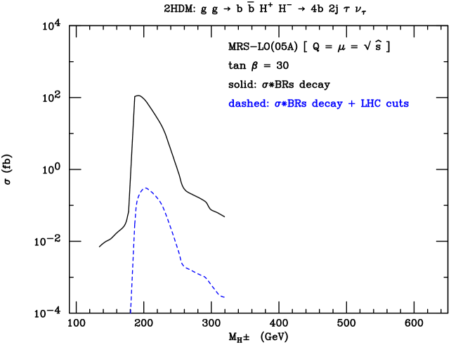
Figure 4: Total cross sections as a function of $M_{H^{\pm}}$ for process (1) yielding the signature (5), including all decay BRs and with finite width effects, before (solid) and after the kinematic cuts in (6)–(10), assuming LHC (dashed) detectors. For reference, the value $\tan\beta=30$ is adopted. The 2HDM described in the text is here assumed.

Under any circumstances, a clear message that emerged from NLO computations of $\bar{b}g\to tH^{+}$ with respect to the LO ones of $gg\to b\bar{t}H^{+}$ is that the former (duly incorporating a running NLO $b$-quark mass in the Yukawa coupling to the charged Higgs boson) agree better with the latter if these use the pole $b$-quark mass instead, see Fig. 4 of Ref. [11]. By analogy, in the reminder of our paper, we will make the same assumption (of a pole $b$-quark mass entering the $b\bar{t}H^{+}$ vertex) in our $gg\to b\bar{b}H^{+}H^{-}$ process at LO. Finally, while a well defined procedure exists in order to compute both inclusive and exclusive cross sections when combining the $b\bar{b}$- and $gg$-initiated processes, through the subtraction of the common logarithm terms [8] and/or by a cut in phase space [9], it should be noticed that process (iv) is the only contributor when one exploits the tagging of both the two $b$-quark jets produced in association with the charged Higgs boson pair.

It is precisely the intention of this note that of pursuing a similar strategy in order to extract a possible $b\bar{b}H^{+}H^{-}$ signal, as it has already been shown the beneficial effects of triggering on the ‘spectator’ $b$-jet in the $gg\to t\bar{b}H^{-}$ case, in order to improve on the discovery reach of charged Higgs bosons at the LHC [16]. Furthermore, if vertices of the type $H^{+}H^{-}\Phi^{0}$ are to be studied experimentally, one should appreciate the importance of the $gg\to b\bar{b}\Phi^{0}$ subprocess (from which two charged Higgs bosons would stem out of the above triple-Higgs coupling: see diagrams $4,8,14,19,23,29,34$ and 38 in Fig. 1) by recalling that the latter reaction is the dominant production mode of neutral Higgs scalars (chiefly, the $H^{0}$ state) at $\tan\beta$ values above 7 or so, for any neutral Higgs mass of phenomenological interest [17], this justifying our choice of privileging here the $gg\to b\bar{b}H^{+}H^{-}$ channel. Finally, whereas the already recalled MSSM relation $M_{H^{\pm}}\simeq M_{A^{0}}\simeq M_{H^{0}}\gg M_{h^{0}}$ clearly prevents the appearance of a $H^{0}\to H^{+}H^{-}$ resonance in the diagrams proceeding via intermediate states of the form $gg\to b\bar{b}H^{0}$, this is no longer true in a general 2HDM, wherein one may well have $M_{H^{0}}>2M_{H^{\pm}}$, with the consequent relative enhancement of the mentioned subset of diagrams with respect to all others appearing in Fig. 1.

We will attempt the signal selection for the case of rather heavy charged Higgs bosons, with masses above that of the top quark. The case for the existence of such massive Higgs states has in fact become phenomenologically pressing, since rumours of a possible evidence of light charged Higgs bosons being produced at LEP2 [18] have faded away. Instead, one is now left from LEP2 with a model independent limit on $M_{H^{\pm}}$, of order $M_{W^{\pm}}$. Within the MSSM, the current lower bound on a light Higgs boson state, of approximately 110 GeV [19], can be converted at two-loops into a minimal value for the charged Higgs boson mass, of order 130–140 GeV, for $\tan\!\beta\,\simeq\,3$–$4$. This bound grows rapidly stronger as $\tan\!\beta$ is decreased while tapering very gradually as $\tan\!\beta$ is increased (staying in the $110$–$125\,\hbox{GeV}$ interval for $\tan\beta\>\raisebox{-2.15277pt}{$\stackrel{{\scriptstyle\textstyle>}}{{\sim}}$}\>7$). Besides, in the mass interval $M_{H^{\pm}}<m_{t}$, charged Higgs bosons could well be found at Tevatron (Run 2) [21], which has already begun data taking at $\sqrt{s}_{p\bar{p}}=2$ TeV at FNAL, by exploiting their production in top decays, $t\to bH^{+}$, and the tau-neutrino detection mode, $H^{-}\to\tau\bar{\nu}_{\tau}$. In contrast, if $M_{H^{\pm}}\>\raisebox{-2.15277pt}{$\stackrel{{\scriptstyle\textstyle>}}{{\sim}}$}\>~{}m_{t}$ (our definition of a ‘heavy’ charged Higgs boson), one will necessarily have to wait for the advent of the LHC, $\sqrt{s}_{pp}=14$ TeV, at CERN. As hinted at in the beginning, we also make the assumption in our study that the charged Higgs boson mass is already known, e.g., from studies of the leading production and decay channels, $gg\to t\bar{b}H^{-}$ and $H^{-}\to\tau^{-}\bar{\nu}_{\tau}$ or $b\bar{t}$, during the first years of running of the CERN hadron machine.

Under the above parameter assumptions, i.e., large $\tan\beta$ ($\>\raisebox{-2.15277pt}{$\stackrel{{\scriptstyle\textstyle>}}{{\sim}}$}\>10$) and large $M_{H^{\pm}}$ values ($\>\raisebox{-2.15277pt}{$\stackrel{{\scriptstyle\textstyle>}}{{\sim}}$}\>m_{t}$), a sensible choice of decay channels [22] for our pair of charged Higgs bosons would be to require one to decay via the leading mode, i.e., $H^{+}\to t\bar{b}$ (with the $t$-quark further decaying hadronically, so to allow for the kinematic reconstruction of the charged Higgs boson resonance in a four-jet system) and the other via $H^{-}\to\tau^{-}\bar{\nu}_{\tau}$ (whose rate increases with $\tan\beta$ and that yields a somewhat cleaner trigger in the LHC environment, independently of whether the $\tau$-lepton decays leptonically or hadronically, as opposed to the above multi-jet and high hadron-multiplicity signature). As such decays would induce an intermediate signal state made up by $b\bar{b}t\bar{b}\tau^{-}\bar{\nu}_{\tau}$ and since we will assume tagging all four $b$’s, it is clear that the dominant irreducible background would be $b\bar{b}t\bar{t}$ production followed by the decay $\bar{t}\to\bar{b}W^{-}\to\bar{b}\tau^{-}\bar{\nu}_{\tau}$.

3 Calculation

The hard subprocess describing our signal is then

$$gg\to b\bar{b}H^{+}H^{-},$$ (1)

whereas for the main irreducible background we have to deal with

$$gg\to b\bar{b}t\bar{t}.$$ (2)

(We neglect here the computation of the quark-antiquark initiated components of both signal and background, i.e., $q\bar{q}\to b\bar{b}H^{+}H^{-}$ and $q\bar{q}\to b\bar{b}t\bar{t}$, respectively, as they are negligible at the LHC, in comparison to the gluon-gluon induced modes.) The matrix elements for (1)–(2) have been calculated by using the HELAS [23] subroutines and MadGraph [24]. All unstable particles entering the two processes ($t,H^{\pm}$ and $W^{\pm}$) were generated not only off-shell (i.e., with their natural widths) but also in Narrow Width Approximation (NWA) for comparison. For the MSSM and 2HDM Higgs bosons, the program HDECAY [25] has been exploited to generate the decays rates eventually used in the Monte Carlo (MC) simulations. For the MSSM, we have assumed the following set up for the relevant SUSY input parameters: $\mu=0$, $A_{\ell}=A_{u}=A_{d}=0$ (with $\ell=e,\mu,\tau$ and $u/d$ referring to $u/d$-type quarks) and $M_{\rm{SUSY}}=1$ TeV, the latter implying a sufficiently heavy scale for all sparticle masses, so that no $H^{\pm}\to$ SUSY decay can take place.

As a 2HDM configuration, we have basically maintained the previous setup in the relevant input parameters of HDECAY, with the most important difference being the assumption of a different relation between the input $M_{A^{0}}$ value and the derived $M_{H^{0}}$ one, by assuming a linear relation between the $H^{0}$ and $H^{\pm}$ masses, i.e., $M_{H^{0}}=x~{}H^{\pm}$, with $x$ being a number larger than 2, while maintaining the MSSM relations among the $H^{\pm}$ and $A^{0}$ masses, thereby allowing for the already intimated onset of $H^{0}\to H^{+}H^{-}$ resonant decays in diagrams $4,8,14,19,23,29,34$ and 38 of Fig. 1. As already remarked upon, this is a crucial phenomenological difference with respect to the MSSM, wherein such a decay threshold is never reached over the unexcluded region of parameter space. Another important difference, in a more general 2HDM, is the value of the triple Higgs coupling $g_{H^{0}H^{+}H^{-}}$ which can be much larger than what is the case in the MSSM.

Before giving the details of the 2HDM setup we are using let us recall the most general CP-conserving 2HDM scalar potential which is symmetric under $\Phi_{1}\to-\Phi_{1}$ up to softly breaking dimension-2 terms (thereby allowing for loop-induced flavour changing neutral currents) [1],

$$V(\Phi_{1},\Phi_{2}) = \lambda_{1}(\Phi_{1}^{\dagger}\Phi_{1}-v_{1}^{2})^{2}+\lambda_{2}(\Phi_{2}^{\dagger}\Phi_{2}-v_{2}^{2})^{2}$$ (3)

$$+\lambda_{3}\left[(\Phi_{1}^{\dagger}\Phi_{1}-v_{1}^{2})+(\Phi_{2}^{\dagger}\Phi_{2}-v_{2}^{2})\right]^{2}$$

$$+\lambda_{4}\left[(\Phi_{1}^{\dagger}\Phi_{1})(\Phi_{2}^{\dagger}\Phi_{2})-(\Phi_{1}^{\dagger}\Phi_{2})(\Phi_{2}^{\dagger}\Phi_{1})\right]$$

$$+\lambda_{5}\left[{\mathrm{Re}}(\Phi_{1}^{\dagger}\Phi_{2})-v_{1}v_{2}\right]^{2}+\lambda_{6}\left[{\mathrm{Im}}(\Phi_{1}^{\dagger}\Phi_{2})\right]^{2}$$

where $v_{1}^{2}+v_{2}^{2}=v^{2}=2M_{W}^{2}/g^{2}\simeq(174$ GeV)². In general, the potential is thus parameterised by seven parameters (the $\lambda_{i}$ and $\tan\beta=v_{2}/v_{1}$) whereas in the MSSM only two of them are independent. In the following we will replace five of the $\lambda_{i}$ with the masses of the Higgs bosons ($M_{h^{0}},M_{H^{0}},M_{A^{0}},M_{H^{\pm}}$) and the mixing angle $\alpha$ of the CP-even Higgs bosons.

From the scalar potential the different three- and four-Higgs couplings can be obtained. (See [26, 27] for a complete compilation of couplings in a general CP-conserving 2HDM.) Using the Higgs masses and $\alpha$ as parameters together with $\lambda_{3}$ the $g_{H^{0}H^{+}H^{-}}$ coupling takes a particularly simple form (see for example [28])

$$g_{H^{0}H^{+}H^{-}} = -i\frac{g}{M_{W}}\left[\cos(\beta-\alpha)\left(M_{H^{\pm}}^{2}-\frac{M_{H^{0}}^{2}}{2}\right)+\frac{\sin(\alpha+\beta)}{\sin 2\beta}\left\{\frac{1}{2}(M_{H^{0}}^{2}+M_{h^{0}}^{2})+\right.\right.$$ (4)

$$\left.\left.+4\lambda_{3}v^{2}-\frac{1}{2\sin 2\beta}\left[\sin 2\alpha+2\sin(\alpha-\beta)\cos(\alpha+\beta)\right](M_{H^{0}}^{2}-M_{h^{0}}^{2})\right\}\right]\>.$$

For the other three- and four-Higgs couplings we refer to [26, 27].

In the 2HDM that we will adopt below we will start from the MSSM parameter values for $M_{H^{0}},M_{A^{0}},M_{h^{0}},M_{H^{\pm}},\tan\beta,\alpha,(\lambda_{5}-\lambda_{6})/2$ using $M_{A^{0}}$ and $\tan\beta$ as input. As already mentioned we then change from $M_{H^{0}}^{\rm MSSM}$ to $M_{H^{0}}^{\rm 2HDM}=2.2M_{H^{\pm}}$ and in addition $M_{h^{0}}=1.7M_{H^{\pm}}$ while keeping the other Higgs boson masses and $\tan\beta$ fixed. The choice $M_{h^{0}}=1.7M_{H^{\pm}}$ has been found to be favourable in order to get a larger $g_{H^{0}H^{+}H^{-}}$ coupling and at the same time avoid negative interference between $H^{0}$ and $h^{0}$ resonances. The remaining two parameters, $\alpha$ and $(\lambda_{5}-\lambda_{6})/2$, are then determined by randomly picking one million ($\alpha,(\lambda_{5}-\lambda_{6})/2$)-points, in the ranges $[-\pi/2,\pi/2]$ and $[-4\pi,4\pi]$ respectively, and keeping the one which gives the largest effective coupling, $g_{H^{0}H^{+}H^{-}}\cos\alpha$, thereby also taking into account the $H^{0}b\bar{b}$-coupling. In order to accept a point we also check that the following conditions are fulfilled: the potential is bounded from below, the $\lambda_{i}$ fulfill the unitarity constraints [29], the contribution to $\Delta\rho<10^{-3}$ (although with the above setup for the Higgs masses we are more or less guaranteed not to violate any experimental bounds on the $\rho$-parameter [1]), and the combined partial width for the three $H^{0}\to h^{0}h^{0},A^{0}A^{0},H^{+}H^{-}$ decays is smaller than $M_{H^{0}}/2$. (We have checked that the partial widths of the $H^{0}\to h^{0}h^{0}h^{0},h^{0}A^{0}A^{0},h^{0}H^{+}H^{-}$ decay channels are negligible.)

Some examples of the actual values of the $\lambda_{i}$ we use in this study are given in Tab. 2 together with the corresponding values of $\alpha$ and $g_{H^{0}H^{+}H^{-}}$. From the table one sees that the effective coupling $g_{H^{0}H^{+}H^{-}}\cos\alpha$ decreases quite rapidly as $M_{A^{0}}$ increases, giving a correspondingly smaller cross-section.(This will be shown in more detail below.) However, it should be kept in mind that the 2HDM setup we are using is not the most general one based on the scalar potential (3) and that there may be other parts of the parameter space which we have not scanned that give a larger cross section. At the same time it should be said that we have already tried different relations between the Higgs masses other than the ones given above, yet we have not made any further detailed investigations.

Table 2: Examples of values of the parameters in the Higgs potential used for different values of $M_{A^{0}}$ together with the corresponding values of $\alpha$ and $g_{H^{0}H^{+}H^{-}}$.

$M_{A^{0}}$	$\lambda_{1}$	$\lambda_{2}$	$\lambda_{3}$	$\lambda_{4}$	$\lambda_{5}$	$\lambda_{6}$	$\alpha$	$g_{H^{0}H^{+}H^{-}}$
$[$GeV$]$								$[$GeV$]$
150	$-$4.81618	$-$4.02795	4.81618	0.941863	4.13114	0.745433	0.5064	$-$1235
200	$-$3.90929	$-$2.75838	3.90929	1.52164	7.16375	1.32521	0.2686	$-$563
250	1.69717	3.17924	$-$1.54105	2.26707	10.9783	2.07065	0.0363	76
300	5.16558	7.63614	$-$3.79044	3.17816	9.19537	2.98173	-1.539	$-$1078

To get an explicit example of the large differences between the more general 2HDM we are considering and the MSSM, we compare the two using $M_{A^{0}}=200$ GeV and $\tan\beta=30$ as input values, as we will do below. In this case we get $g_{H^{0}H^{+}H^{-}}^{\rm 2HDM}=-563$ GeV in the 2HDM instead of the MSSM value, $g_{H^{0}H^{+}H^{-}}^{\rm MSSM}=-1.8$ GeV. With the value of $\alpha^{\rm 2HDM}=0.26859$ not being much larger than $\alpha^{\rm MSSM}=-0.05774$ the difference in effective coupling $g_{H^{0}H^{+}H^{-}}\cos\alpha$ is more than a factor hundred and as we will see below it has a large impact on the magnitude of the cross section. (The $H^{0}$ widths will of course be different too in the MSSM and 2HDM just described: their effects have been included in the numerical analysis.)

As intimated already in Sect. 2, a non-running $b$-quark mass was adopted for both the kinematics and the Yukawa couplings: $m_{b}=4.25$ GeV. For the top parameters, we have taken $m_{t}=175$ GeV with $\Gamma_{t}$ computed according to the model used (in the limit $M_{H^{\pm}}\gg m_{t}$, we have $\Gamma_{t}=1.56$ GeV in both the 2HDM and MSSM scenarios considered here). EW parameters were as follows: $\alpha_{\rm{EM}}=1/128$, $\sin^{2}\theta_{W}=0.232$, with $M_{Z^{0}}=91.19$ GeV ($\Gamma_{Z^{0}}=2.50$ GeV) and $M_{W^{\pm}}=M_{Z^{0}}\cos\theta_{W}$ ($\Gamma_{W^{\pm}}=2.08$ GeV). For the $\tau$-lepton mass we used $m_{\tau}=1.78$ GeV, whereas all the other leptons and quarks were assumed to be massless.

The integrations over the multi-body final states have been performed numerically with the aid of VEGAS [30], Metropolis [31] and RAMBO [32], for checking purposes. Finite calorimeter resolution has been emulated through a Gaussian smearing in transverse momentum, $p^{T}$, with $(\sigma(p^{T})/p^{T})^{2}=(0.60/\sqrt{p^{T}})^{2}+(0.04)^{2}$ for all jets and $(\sigma(p^{T})/p^{T})^{2}=(0.12/\sqrt{p^{T}})^{2}+(0.01)^{2}$ for leptons. The corresponding missing transverse momentum, $p^{T}_{\mathrm{miss}}$, was reconstructed from the vector sum of the visible momenta after resolution smearing. Furthermore, we have identified jets with the partons from which they originate and applied all cuts directly to the latter, since parton shower and hadronisation were not included in our study. The only exception is the $\tau$-lepton decay which has been taken into account using the Pythia [33] MC event generator.

As default PDFs we have adopted the set MRS98LO(05A) [34] with $Q=\mu=\sqrt{\hat{s}}$ as factorisation/renormalisation scale for both signal and background. The same scale entered the evolution of $\alpha_{{\rm S}}$, which was performed at one-loop, with a choice of $\Lambda_{\rm{QCD}}^{n_{f}=4}$ consistent with the PDF set adopted. In fact, we have verified that the spread in the inclusive cross sections, for both signal and background, as obtained by using the five different parameterisations of MRS98LO and also CTEQ4L [34] was within $6-7\%$ of the values quoted for MRS98LO(05A) in the remainder of the paper.

4 Selection

The signature that we are then considering is in practice:

$$4~{}b{\rm{-jets}}~{}+~{}2~{}{\rm{light-jets}}~{}+~{}\tau~{}+~{}p^{T}_{\rm{miss}},$$ (5)

wherein the two $b$-jets from the hard process are actually defined as the two most forward/backward ones that also display a displaced vertex.

We have assumed a standard detector configuration by imposing acceptance and separation cuts on all light-quark (including $c$’s) and $b$-jets, labeled as $j$ and $b$, respectively, as follows:

$$p^{T}_{b}>20~{}{\rm{GeV}},\qquad|\eta_{b}|<2.5,\qquad p^{T}_{j}>20~{}{\rm{GeV}},\qquad|\eta_{j}|<5,\qquad\Delta R_{jj,jb}>0.4.$$ (6)

The two most forward/backward $b$-jets (with pseudorapidities of opposite sign) are further required to yield

$$M_{bb}>M_{H^{\pm}}$$ (7)

for their invariant mass. For $\tau$-jets (we only consider hadronic decay modes) we impose:

$$p^{T}_{\tau}>10~{}{\rm{GeV}},\qquad\qquad|\eta_{\tau}|<2.5,\qquad\qquad\Delta R_{j\tau,b\tau}>0.4.$$ (8)

The setup corresponds to the standard ATLAS/CMS detectors. Presently it is not clear to what extent this setup will also be applicable for the same apparata in the context of the Super LHC (SLHC) option [35].

Having now excluded the two most forward/backward $b$-jets from the list of jets, we impose hadronic $W^{\pm}$- and $t$-mass reconstruction:

$$|M_{jj}-M_{W^{\pm}}|<15~{}{\rm{GeV}},\qquad\qquad|M_{bjj}-m_{t}|<35~{}{\rm{GeV}},$$ (9)

where the two light-quark jets entering the last inequality are of course the same fulfilling the first one. Finally, the missing transverse momentum should be:

$$p^{T}_{\rm{miss}}>60~{}{\rm{GeV}}.$$ (10)

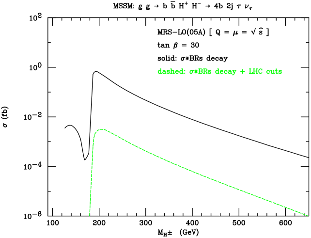
Figure 3: Total cross sections as a function of $M_{H^{\pm}}$ for process (1) yielding the signature (5), including all decay BRs and with finite width effects, before (solid) and after the kinematic cuts in (6)–(10), assuming LHC (dashed) detectors. For reference, the value $\tan\beta=30$ is adopted. The MSSM described in the text is here assumed.

The combined effects of these cuts on the signal (1) in the MSSM and 2HDM models is shown in Figs. 3 and 4 respectively in the case of retaining the finite width effects using off-shell masses for the $H^{\pm}$ and $W^{\pm}$. (The difference when instead using the NWA is very small and this option is therefore not shown.) As can be seen from the figures the effects of the cuts on the magnitude of the cross sections is quite severe. On the other hand the cuts are needed (especially in case of the MSSM) in order to beat down the background as is illustrated in Fig. 5. From the figure it is also clear that the signal cross section reaches its maximum around $M_{H^{\pm}}=200$ GeV and that the magnitude of the signal varies by up to 2 orders of magnitude depending on which model we are considering. It should also be noted that in the 2HDM setup we are using it was not possible to go above $M_{H^{\pm}}\simeq 320$ GeV (corresponding to $M_{H^{0}}=700$ GeV) due to the unitarity contraints [29]. In the following we will be considering the case $M_{H^{\pm}}\simeq 215$ GeV (corresponding to $M_{A^{0}}=200$ GeV) in more detail.

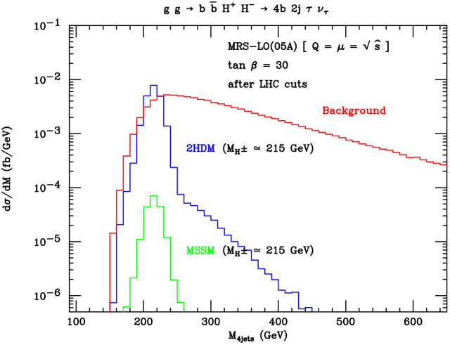
Figure 6: Differential distribution in the invariant mass of the ‘four-jet system’ defined in the text for processes (1) (with finite width effects) and (2) yielding the signature (5), including all decay BRs and after the kinematic cuts in (6)–(10), assuming LHC detectors. For reference, the values $M_{H^{\pm}}=215$ GeV and $\tan\beta=30$ are adopted. The MSSM and the 2HDM described in the text are here compared to the background.

After the above cuts have been implemented and the jet momenta assigned, one can reconstruct the would-be charged Higgs boson mass, by pairing the three jets entering the equation in the right-hand side of (9) with the left-over central jet, a quantity which we denote by $M_{4{\rm{jets}}}$. The corresponding mass spectrum is presented in Fig. 6 for our two customary setups of MSSM and 2HDM, assuming $M_{H^{\pm}}=215$ GeV and $\tan\beta=30$ as representative values. The figure shows clear peaks at the charged Higgs boson mass for the signal on top of a combinatorial background in both models whereas for the background process there is no such peak. Thus, by selecting events with

$$180~{}\mathrm{GeV}<M_{4{\rm{jets}}}<250~{}\mathrm{GeV}$$ (11)

we can get an additional discrimination against the background.

Furthermore, using the visible $\tau$-jet momentum and the missing transverse one, it is possible to reconstruct the transverse mass, as

$$M^{T}_{\tau\nu_{\tau}}=\sqrt{2p_{\tau}p^{T}_{\rm{miss}}(1-\cos\Delta\phi)},$$ (12)

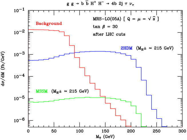
Figure 7: Differential distribution in transverse mass of the ‘tau-neutrino’ system defined in the text for processes (1) (with finite width effects) and (2) yielding the signature (5), including all decay BRs and after the kinematic cuts in (6)–(10), assuming LHC detectors. For reference, the values $M_{H^{\pm}}=215$ GeV and $\tan\beta=30$ are adopted. The MSSM and the 2HDM described in the text are here compared to the background.

with $\Delta\phi$ the relative angle between the two momenta, a quantity which is ultimately correlated to the actual value of the mass resonance yielding $\tau^{-}\bar{\nu}_{\tau}$ pairs ($H^{-}$ in the signal and $W^{-}$ in the background). We show this observable in Fig. 7 (where it is denoted by $M_{T}$), again, for our two customary setups of MSSM and 2HDM. From the figure it is clear that the transverse mass for the signal in the two models extends all the way out to $\sim M_{H^{\pm}}$. Comparing with the background, which starts to drop quite drastically around $M^{T}_{\tau\nu_{\tau}}\approx M_{W^{\pm}}$, we see that it is advantageous to introduce a cut on the transverse mass of the order of

$$M^{T}_{\tau\nu_{\tau}}>M_{H^{\pm}}/2~{}(\simeq 107~{}\mathrm{GeV}).$$ (13)

This gives a very strong suppression of the background whereas the signal is only mildly affected.

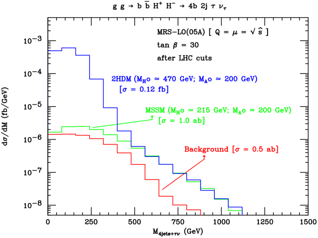
Figure 8: Differential distribution in transverse mass of the ‘four-jets plus tau-neutrino’ system defined in the text for processes (1) (with finite width effects) and (2) yielding the signature (5), including all decay BRs and after the kinematic cuts in (6)–(11) and (13), assuming LHC detectors. For reference, the values $M_{H^{\pm}}=215$ GeV and $\tan\beta=30$ are adopted. The MSSM and the 2HDM described in the text are here compared to the background.

After having reconstructed the two charged Higgs bosons and applied the respective cuts (11) and (13) we can form the (effectively, transverse) mass $M^{T}_{{\rm{4jets}}+\tau\nu}$ of the combined two charged Higgs boson system, giving the possibility to look for possible resonances. As can be seen from the magnitudes of the cross sections in Fig. 8 the selection outlined above gives a very clear signal in the 2HDM case with essentially no background, whereas in the MSSM case the signal is still clear but very small. Of course, the cuts could be tightend to give a very clear signal also in the MSSM case, but the absolute cross section would then be even smaller. From the figure it is also clear that there is a significant difference in shape between the two models, with the 2HDM showing a clear enhancement for $M^{T}_{{\rm{4jets}}+\tau\nu}\>\raisebox{-2.15277pt}{$\stackrel{{\scriptstyle\textstyle<}}{{\sim}}$}\>500$ GeV due to the resonant contributions. However, given the limited statistics that will be available at the LHC, it is not clear to what extent the difference in shape alone can be used to extract any information about possible $H^{0}\to H^{+}H^{-}$ resonances and the corresponding coupling. In addition the difference in shape will be smaller if the width of the $H^{0}$ Higgs boson is larger and/or the detector resolution is worse than what we have assumed.

5 Conclusion

As we have shown, it is possible to outline a selection procedure that enables one to extract a signal of heavy charged Higgs pair production in association with two $b$-quarks at $\tan\beta\>\raisebox{-2.15277pt}{$\stackrel{{\scriptstyle\textstyle>}}{{\sim}}$}\>30$ in extensions of the standard model with two Higgs doublets of Type II. In a general case the mass relations in the Higgs sector may be favourable such that a sizeable signal would appear already at the LHC through the resonant channel $gg\to b\bar{b}H^{0}\to b\bar{b}H^{+}H^{-}$. However, in the MSSM the resonance is not accessible over the allowed parameter region and the non-resonant contributions turn out to be very small making it difficult to extract a signal even after upgrading the luminosity at LHC by a factor ten (SLHC). The large difference in cross section between the MSSM and a more general 2HDM shows that indeed the pair production of charged Higgs production is sensitive to the $H^{0}H^{+}H^{-}$ coupling even though it will probably be difficult to reconstruct a resonant transverse mass peak mainly due to the limited statistics and possibly also due to the finite detector resolution.

In our study we have not included effects of the $b$-tagging efficiency. On the one hand, requiring four $b$-tags will give a sizeable reduction (of the order of a factor ten) of the signal as well as the backgrounds. On the other hand, the selection procedure outlined above was designed to get a signal in the case of the MSSM leading to unnecessarily tight cuts for the general 2HDM case. Furthermore, being a leading order calculation, the cross section we get for the signal is also sensitive to the choice of factorisation and renormalisation scales. If we, instead of using the standard choice of the invariant mass of the hard subsystem, use the mean transverse mass of the two $b$-quarks in the $gg\to b\bar{b}H^{+}H^{-}$ process as scale, the cross section increases by a factor 5. Such a scale choice also gives a better agreement with the cross section for the ‘twin’ process $b\bar{b}\to H^{+}H^{-}$. In order to get a better handle on the uncertainties due to scale choices a next-to-leading order calculation will eventually be necessary. Nonetheless, we believe that our results already call for the attention of ATLAS and CMS in further exploring the scope of the (S)LHC in reconstructing the form of the Higgs potential in extended models through signals of charged Higgs boson pairs. Besides, in presence of parton shower, hadronisation and detector effects, one may also realistically attempt exploiting $\tau$-polarisation techniques in hadronic decays of the heavy lepton [36] in order to increase the signal-to-background rates, an effort that was beyond the scope of our parton level analysis.

Figure 1: Feynman diagrams in the unitary gauge for process (1).

Figure 1: continued

Figure 1: continued

References

- [1] J.F. Gunion, H.E. Haber, G.L. Kane and S. Dawson, “The Higgs Hunter Guide” (Addison-Wesley, Reading MA, 1990), Erratum, hep-ph/9302272.
- [2] D.A. Dicus, J.L. Hewett, C. Kao and T.G. Rizzo, Phys. Rev. D 40, 787 (1989); J.F. Gunion, Phys. Lett. B 322, 125 (1994); V. Barger, R.J.N. Phillips and D.P. Roy, Phys. Lett. B 324, 236 (1994); S. Raychaudhuri and D.P. Roy, Phys. Rev. D 52, 1556 (1995), ibid. D 53, 4902 (1996); S. Moretti and K. Odagiri, Phys. Rev. D 55, 5627 (1997), ibid. D 59, 055008 (1999); D.P. Roy, Phys. Lett. B 459, 607 (1999); S. Moretti and D.P. Roy, Phys. Lett. B 470, 209 (1999); M. Drees, M. Guchait and D.P. Roy, Phys. Lett. B 471, 39 (1999); F. Borzumati, J.-L. Kneur and N. Polonsky, Phys. Rev. D 60, 115011 (1999); K. Odagiri, hep-ph/9901432; A.A. Barrientos Bendezú and B.A. Kniehl, Phys. Rev. D 59, 015009 (1999), ibid. D 61, 097701 (2000), ibid. D 63, 015009 (2001); D.J. Miller, S. Moretti, D.P. Roy and W.J. Stirling, Phys. Rev. D 61, 055011 (2000); S. Moretti, Phys. Lett. B 481, 49 (2000); O. Brein, W. Hollik and S. Kanemura, Phys. Rev. D 63, 095001 (2001). For recent experimental studies and reviews, see: K.A. Assamagan, ATL–PHYS–99–013 and ATL–PHYS–99–025; K.A. Assamagan and Y. Coadou, ATL–COM–PHYS–2000–017; K.A. Assamagan et al., hep-ph/0002258; K.A. Assamagan, Y. Coadou and A. Deandrea, Eur. Phys. J. direct C9, 1 (2002).
- [3] M. Bisset, M. Guchait and S. Moretti, Eur. Phys. J. C 19, 143 (2001); K.A. Assamagan, M. Bisset, Y. Coadou, A.K. Datta, A. Deandrea, A. Djouadi, M. Guchait, Y. Mambrini, F. Moortgat and S. Moretti, in hep-ph/0203056; S. Moretti, proceedings of the ‘Seventh Workshop on High Energy Physics Phenomenology WHEPP-VII’, Harish Chandra Research Institute, Allahabad, India, 4-15 January 2002, hep-ph/0205104; A. Datta, A. Djouadi, M. Guchait and F. Moortgat, hep-ph/0303095; M. Bisset, F. Moortgat and S. Moretti, hep-ph/0303093; A. Datta, A. Djouadi, M. Guchait and Y. Mambrini, Phys. Rev. D 65, 015007 (2002); H. Baer, M. Bisset, X. Tata and J. Woodside, Phys. Rev. D 46, 303 (1992).
- [4] S. Moretti, J. Phys. G 28, 2567 (2002).
- [5] E. Eichten, I. Hinchliffe, K. Lane and C. Quigg, Rev. Mod. Phys. 56, 579 (1984).
- [6] S.S.D. Willenbrock, Phys. Rev. D 35, 173 (1987); Y. Jiang, W.-G. Ma, L. Han, M. Han and Z.-H. Yu, J. Phys. G 23, 385 (1997), Erratum, ibidem G 23, 1151 (1997); A. Krause, T. Plehn, M. Spira and P.M. Zerwas, Nucl. Phys. B 519, 85 (1998); A. Belyaev, M. Drees, O.J.P. Eboli, J.K. Mizukoshi and S.F. Novaes, Phys. Rev. D 60, 075008 (1999); A. Belyaev, M. Drees and J.K. Mizukoshi, Eur. Phys. J. C 17, 337 (2000); A.A. Barrientos Bendezú and B.A. Kniehl, Nucl. Phys. B568, 305 (2000); O. Brein and W. Hollik, Eur. Phys. J. C 13, 175 (2000).
- [7] S.H. Zhu, Phys. Rev. D 67, 075006 (2003).
- [8] F. Borzumati, J.-L. Kneur and N. Polonsky, in Ref. [2].
- [9] A. Belyaev, D. Garcia and J. Guasch and J. Sola, Phys. Rev. D 65, 031701 (2002), JHEP 06, 059 (2002).
- [10] S. Moretti and D.P. Roy, in Ref. [2].
- [11] T. Plehn, Phys. Rev. D 67, 014018 (2003).
- [12] F. Maltoni, Z. Sullivan and S. Willenbrock, Phys. Rev. D 67, 093005 (2003).
- [13] E. Boos and T. Plehn, hep-ph/0304034.
- [14] R. V. Harlander and W. B. Kilgore, hep-ph/0304035.
- [15] D. Cavalli et al., in hep-ph/0203056.
- [16] D.J. Miller, S. Moretti, D.P. Roy and W.J. Stirling, in Ref. [2].
- [17] M. Spira, Fortsch. Phys. 46, 203 (1998).
- [18] See, e.g.: M. Antonelli and S. Moretti, hep-ph/0106332 (and references therein).
- [19] See, e.g.: LEP HIGGS Working Group web page, http://www.cern.ch/LEPHIGGS/.
- [20] A. Brignole, J. Ellis, G. Ridolfi and F. Zwirner, Phys. Lett. B 271, 123 (1991); A. Brignole, Phys. Lett. B 277, 313 (1992); M.A. Díaz and H.E. Haber, Phys. Rev. D 45, 4246 (1992).
- [21] M. Carena, J.S. Conway, H.E. Haber and J.D. Hobbs (conveners), proceedings of the ‘Tevatron Run II SUSY/Higgs’ Workshop, Fermilab, Batavia, Illinois, USA, February-November 1998, hep-ph/0010338; M. Guchait and S. Moretti, JHEP 01, 001 (2002).
- [22] S. Moretti and W.J. Stirling, Phys. Lett. B 347, 291 (1995), Erratum, ibidem B 366, 451 (1996); A. Djouadi, J. Kalinowski and P.M. Zerwas, Z. Phys. C 70, 435 (1996); E. Ma, D.P. Roy and J. Wudka, Phys. Rev. Lett. 80, 1162 (1998).
- [23] H. Murayama, I. Watanabe and K. Hagiwara, KEK Report 91–11, January 1992.
- [24] T. Stelzer and W.F. Long, Comput. Phys. Commun. 81, 357 (1994).
- [25] A. Djouadi, J. Kalinowski and M. Spira, Comp. Phys. Comm. 108, 56 (1998).
- [26] F. Boudjema and A. Semenov, Phys. Rev. D 66, 095007 (2002).
- [27] J. F. Gunion and H. E. Haber, Phys. Rev. D 67, 075019 (2003).
- [28] A. Arhrib and G. Moultaka, Nucl. Phys. B 558, 3 (1999).
- [29] A. G. Akeroyd, A. Arhrib and E. M. Naimi, Phys. Lett. B 490, 119 (2000).
- [30] G.P. Lepage, Jour. Comp. Phys. 27, 192 (1978).
- [31] H. Kharraziha and S. Moretti, Comp. Phys. Comm. 127, 242 (2000), Erratum, ibidem B 134, 136 (2001).
- [32] R. Kleiss, W.J. Stirling and S.D. Ellis, Comput. Phys. Commun. 40, 359 (1986).
- [33] T. Sjöstrand, P. Eden, C. Friberg, L. Lönnblad, G. Miu, S. Mrenna and E. Norrbin, Comput. Phys. Commun. 135, 238 (2001).
- [34] See http://durpdg.dur.ac.uk/hepdata/pdf.html for an up-to-date compilation of PDFs.
- [35] F. Gianotti, M.L. Mangano, T. Virdee (conveners), hep-ph/0204087.
- [36] S. Raychaudhuri and D. P. Roy, second paper in Ref. [2].