Chiral fermion mass and dispersion relations at finite temperature in the presence of hypermagnetic fields

Abstract

We study the modifications to the real part of the thermal self-energy for chiral fermions in the presence of a constant external hypermagnetic field. We compute the dispersion relation for fermions occupying a given Landau level to first order in ${g^{\prime}}^{2}$, $g^{2}$ and $g_{\phi}^{2}$ and to all orders in $g^{\prime}B$, where $g^{\prime}$ and $g$ are the U(1)_Y and SU(2)_L couplings of the standard model, respectively, $g_{\phi}$ is the fermion Yukawa coupling, and $B$ is the hypermagnetic field strength. We show that in the limit where the temperature is large compared to $\sqrt{g^{\prime}B}$, left- and right-handed modes acquire finite and different $B$-dependent masses due to the chiral nature of their coupling with the external field. Given the current bounds on the strength of primordial magnetic fields, we argue that the above is the relevant scenario to study the effects of magnetic fields on the propagation of fermions prior and during the electroweak phase transition.

I Introduction

The study of the origin and properties of large scale magnetic fields has become a subject of intense research over the last years Reviews . Experimental bounds on their strength can be set for astrophysical objects whose local electron density and spatial structure is known or can be estimated Kron ; Beck . For example, in the case of our galaxy, both quantities are reasonably well known and the average field strength $B$ has been measured to be on the order of 3 - 4 $\mu$G. Several other spiral galaxies in the local group contain magnetic fields of similar intensities. At larger scales, only model dependent upper limits can be established. These limits are also in the few $\mu$G range. In the intracluster medium, recent results have shown the existence of $\mu$G magnetic fields Eilek ; Clarke . For intergalactic large scale fields (dissociated from any particular galaxy or cluster of galaxies), an upper bound of $10^{-9}$G has been estimated by taking reasonable values for the magnetic coherence length Kron .

The origin of these fields is nowadays unknown but it is widely accepted that in order to generate them, two important ingredients are needed: a mechanism for creating the seed fields and a process for amplifying both their amplitude and their coherence scale Reviews ; Giovannini1 . Generation of the seed field may be either primordial or associated to the process of structure formation. During the evolution of the early universe there are a number of proposed mechanisms that could possibly generate primordial magnetic fields. Among the best suited are first order phase transitions Quash ; Baym ; Boyan , which provide favorable conditions for magnetogenesis such as charge separation, turbulence and out-of-equilibrium conditions.

Independently of their origin, the presence of primordial magnetic fields during the evolution of the early universe could have had important consequences on some cosmological phenomena. For instance, magnetic fields can influence big bang nucleosynthesis, thus affecting the primordial abundance of light elements and the rate of expansion of the universe.

Recall that within the standard model (SM) and prior to the electroweak phase transition (EWPT), the only magnetic modes able to propagate for large distances belonged to the (Abelian) U(1)_Y group and are therefore properly called hypermagnetic fields. Non-Abelian magnetic fields develop a magnetic mass through interactions in the electroweak plasma and are thus screened. Consequently, fermions coupled chirally to the magnetic fields through their weak hypercharge. It has recently been shown that the chiral nature of this coupling is directly responsible for the building up of an axial asymmetry during the scattering of fermions with the bubbles of a first order EWPT Ayala1 ; Ayala2 . Another interesting question is to what extent the hypermagnetic fields affected the thermal properties of these chiral fermions prior to the EWPT. This is the issue we take up in this article. In particular, we study the modification to the mass and dispersion relation of these chiral fermions in the presence of a constant hypermagnetic field.

This question has been recently explored in Refs. Cannellos , in the limit where $\sqrt{g^{\prime}B}$ is large compared to the temperature, where $g^{\prime}$ is the U(1)_Y coupling constant. Nevertheless, for homogeneous fields, under the assumption of adiabatic amplification, the current bound $B_{0}\sim 10^{-9}\$G set by the COBE measurement of temperature anisotropies Barrow , gives an upper limit $g^{\prime}B\leq T^{2}$, at the EWPT. However, there is no direct bound on the magnetic energy density as long as this is much smaller than the radiation energy density, and this condition is satisfied for $T\gg\sqrt{g^{\prime}B}$. In any case, the current observations seem to favor the scenario in which $T$ is larger –if not much larger– than $\sqrt{g^{\prime}B}$, prior to and during the EWPT.

Figure 1: Feynman diagrams contributing to the chiral fermion self-energy at one loop.

In this work we compute the self-energies for left- and right-handed fermions in the relevant context of the SM for temperatures prior to the EWPT in the presence of hypermagnetic fields. We use Schwinger’s proper time method Schwinger ; Sahu to incorporate the effects of the external field to all orders in $g^{\prime}B$ in the propagators and work at one loop level. By considering the limit $T\gg\sqrt{g^{\prime}B}$ we find the dispersion relations for these fermions. We show that for a given Landau level, these modes acquire finite and different $B$-dependent thermal masses due to the chiral nature of the fermion coupling to the hypermagnetic field. We also find the mass splitting between particle and collective (hole) excitations. In terms of the kinematice regimes of temperature and magnetic fields, our work compliments the one in Ref. Cannellos .

The work is organized as follows: In Sec. II we compute the finite temperature fermion self-energies at one-loop in the presence of an external hypermagnetic field using Schwinger’s proper time method. In Sec. III, we work in the weak field limit and in Sec. IV we further consider the high-temperature limit. In Sec. V we find the mass and dispersion relations for left- and right-handed modes. Although the sample calculation presented there has been worked out for the top quark alone, the formalism presented is general and can be readily applied to the case of any SM fermion. We summarize and discuss our results in Sec. VI.

II Chiral fermion self-energies in a constant hypermagnetic field

The Feynman diagrams contributing to the one-loop left- and right-handed fermion self energies in the symmetric phase of the SM are depicted in Fig. 1. Figures 1($c$) and ($d$) represent the contributions from internal Higgs boson lines and are thus proportional to $g^{2}_{\phi}$, where $g_{\phi}$ is the Yukawa coupling for the given fermion species. Since the Yukawa couplings and the vacuum masses of fermions are proportional to each other, the contribution from these diagrams is only significant for the top quark for which $g_{\phi}\sim{\mathcal{O}}(1)$. Since we are interested in describing the thermal properties of fermions propagating in the early universe where the particle antiparticle asymmetry is small, we consider that the chemical potential vanishes and thus that there is no contribution to the self-energies from tadpole diagrams.

In order to consider the effect of the external field to all orders in $\sqrt{g^{\prime}B}$, we need to write the exact propagators in the presence of a constant hypermagnetic field. Notice that gauge boson propagators in the internal lines of Fig. 1 $(a)$ and $(b)$ do not couple to an external U(1)_Y field and thus do not need to be dressed by the effects of this field. We take ${\mathbf{B}}$ oriented in the $\hat{z}$ direction. Using Schwinger’s proper-time method, it is possible to obtain the exact expressions for the vacuum propagators of the massless (hyper)charged fermion and scalar-boson, $S_{0}(x^{\prime},x^{\prime\prime})$ and $D_{0}(x^{\prime},x^{\prime\prime})$, respectively

$$\!\!\!\!S_{0}(x^{\prime},x^{\prime\prime}) = \phi(x^{\prime},x^{\prime\prime})\int\frac{d^{4}k}{(2\pi^{4})}e^{-ik\cdot(x^{\prime}-x^{\prime\prime})}S_{0}(k)$$

$$\!\!\!\!D_{0}(x^{\prime},x^{\prime\prime}) = \phi^{*}(x^{\prime},x^{\prime\prime})\int\frac{d^{4}k}{(2\pi^{4})}e^{-ik\cdot(x^{\prime}-x^{\prime\prime})}D_{0}(k),$$ (1)

where $S_{0}(k)$ and $D_{0}(k)$ are given by

$$iS_{0}(k) \equiv \int_{0}^{\infty}\frac{ds}{\cos z}\exp\left[is\left(k_{||}^{2}-k_{\perp}^{2}\ \frac{\tan z}{z}\right)-\epsilon|s|\right]\left\{k\;\!\!\!\!\!\!\!\!\not\,\,\,\,_{||}e^{iz\Sigma_{3}}-\frac{k\;\!\!\!\!\!\!\!\!\not\,\,\,\,_{\perp}}{\cos z}\right\}$$

$$iD_{0}(k) \equiv \int_{0}^{\infty}\frac{ds}{\cos\tilde{z}}\exp\left[is\left(k_{||}^{2}-k_{\perp}^{2}\ \frac{\tan\tilde{z}}{\tilde{z}}\right)-\epsilon|s|\right]\,,$$ (2)

where for simplicity we write $z=g^{\prime}YBs$ and $\tilde{z}=Y_{\phi}Bs/2$, with $Y=Y^{R,L}/2$ the hypercharge for the left- or right-handed mode of the given fermion species, and $Y_{\phi}$ the hypercharge for the boson field. Also, in Eq. (2) we use the definitions

$$(a\cdot b)_{||} = a^{0}b^{0}-a^{3}b^{3}$$

$$(a\cdot b)_{\perp} = a^{1}b^{1}+a^{2}b^{2}\,,$$ (3)

and

$$\Sigma_{3}\equiv\sigma^{12}=\frac{i}{2}[\gamma^{1},\gamma^{2}]=\left(\begin{array}[]{cc}\sigma_{3}&0\\ 0&\sigma_{3}\end{array}\right)\,.$$ (6)

The vacuum gauge boson propagator is simply given by

$$G_{0}^{\mu\nu}(q)=-\frac{1}{q^{2}+i\epsilon}\left[g^{\mu\nu}-\left(1-\frac{1}{\xi}\right)\frac{q^{\mu}q^{\nu}}{q^{2}}\right]\,,$$ (7)

where $\xi$ is the gauge-fixing parameter. The phase factor $\phi$ in Eqs. (1) is given by

$$\phi(x^{\prime},x^{\prime\prime})=\exp\left[ig^{\prime}Y\int_{x^{\prime\prime}}^{x^{\prime}}dx_{\mu}A^{\mu}(x)\right]\,.$$ (8)

and does not depend on the integration path. It depends however on the choice of the residual gauge freedom. We work in the symmetric gauge $A_{\mu}=-\frac{\mbox{\small}{1}}{\mbox{\small}{2}}F_{\mu\nu}x^{\nu}$ and thus

$$\phi(x^{\prime},x^{\prime\prime})=\exp\left(i\frac{g^{\prime}Y}{2}{x_{\mu}}^{\prime\prime}F^{\mu\nu}{x^{\prime}}_{\nu}\right)\,.$$ (9)

We use the real-time formulation of thermal field theory, writing the fermion, scalar-boson and gauge-boson propagators at finite temperature as

$$S(x^{\prime},x^{\prime\prime}) = \phi(x^{\prime},x^{\prime\prime})\int\frac{d^{4}k}{(2\pi^{4})}e^{-ik\cdot(x^{\prime}-x^{\prime\prime})}S(k)$$

$$D(x^{\prime},x^{\prime\prime}) = \phi^{*}(x^{\prime},x^{\prime\prime})\int\frac{d^{4}k}{(2\pi^{4})}e^{-ik\cdot(x^{\prime}-x^{\prime\prime})}D(k)$$

$$G(x^{\prime},x^{\prime\prime}) = \int\frac{d^{4}k}{(2\pi^{4})}e^{-ik\cdot(x^{\prime}-x^{\prime\prime})}G(k)\,,$$ (10)

where

$$S(k) = S_{0}(k)-\tilde{n}_{F}(k_{0})[S_{0}(k)-\bar{S}_{0}(k)]$$

$$D(k) = D_{0}(k)+n_{B}(k_{0})[D_{0}(k)-D_{0}^{*}(k)]$$

$$G^{\mu\nu}(k) = G^{\mu\nu}_{0}(k)+n_{B}(k_{0})[G^{\mu\nu}_{0}(k)-G^{\mu\nu*}_{0}(k)]\,.$$ (11)

In Equations (11), $\tilde{n}_{F}(k_{0})=\tilde{n}(k_{0})\theta(k_{0})+\tilde{n}(-k_{0})\theta(-k_{0})$ and $n_{B}=n(k_{0})\theta(k_{0})+n(-k_{0})\theta(-k_{0})$ where

$$\tilde{n}(k_{0}) = \frac{1}{e^{k_{0}/T}+1}$$

$$n(k_{0}) = \frac{1}{e^{k_{0}/T}-1}\,$$ (12)

are the Fermi-Dirac and Bose-Einstein distributions, respectively. In analogy to Eqs. (10), the corresponding expression for the fermion self-energy is given by

$$\Sigma(x^{\prime},x^{\prime\prime})=\phi(x^{\prime},x^{\prime\prime})\int\frac{d^{4}k}{(2\pi^{4})}e^{-ik\cdot(x^{\prime}-x^{\prime\prime})}\Sigma(k)\,.$$ (13)

The contribution to the fermion self-energy stemming from the exchange of gauge bosons, depicted in Figs. 1($a$) and ($b$) can be generically written as

$$-i\Sigma^{\mbox{\tiny{gauge}}}(k)=iG^{2}\int\frac{d^{4}p}{(2\pi)^{4}}\left\{\begin{array}[]{c}R\\ 1\end{array}\right\}\gamma_{\mu}S(p)G^{\mu\nu}(q)\gamma_{\nu}\left\{\begin{array}[]{c}L\\ 1\end{array}\right\}\,,$$ (18)

where $R=\frac{\mbox{\small}{1}}{\mbox{\small}{2}}(1+\gamma_{5})$, $L=\frac{\mbox{\small}{1}}{\mbox{\small}{2}}(1-\gamma_{5})$ and $G$ stands for $\frac{\mbox{\small}{g}}{\mbox{\small}{2}}$ or $g^{\prime}Y$. The upper row in Eq. (18) refers to the case where the external fermion is left-handed and the lower row corresponds to the case where the external fermion is right-handed. On the other hand, the contribution to the fermion self-energy coming from the exchange of a scalar boson, depicted in Figs. 1 $(c)$ and $(d)$ can be generically written as

$$-i\Sigma^{\mbox{\tiny{scalar}}}(k)=g_{\phi}^{2}\int\frac{d^{4}p}{(2\pi)^{4}}S(p)D(q)\,,$$ (19)

In Eqs. (18) and (19), $q=k-p$.

Since we are interested in computing the dispersion relation, we look at the real parts of Eqs. (18) and (19) and thus

$$i\int\frac{d^{4}p}{(2\pi)^{4}}\gamma_{\mu}S(p)G^{\mu\nu}(q)\gamma_{\nu}\rightarrow\Sigma_{W}(k)+\Sigma_{f}(k)$$

$$i\int\frac{d^{4}p}{(2\pi)^{4}}S(p)D(q)\rightarrow\Sigma_{\phi}(k)+\Sigma_{f\phi}(k)\,,$$ (20)

where we have defined

$$\Sigma_{W}(k)\!\! \equiv \!\!-2\pi\int\!\!\frac{d^{4}p}{(2\pi)^{4}}\gamma_{\mu}S_{0}(p)\gamma^{\mu}\delta(q^{2})n_{B}(q)$$

$$\Sigma_{f}(k)\!\! \equiv \!\!i\int\!\!\frac{d^{4}p}{(2\pi)^{4}}\gamma_{\mu}\frac{[S_{0}(p)-\bar{S}_{0}(p)]}{q^{2}+i\epsilon}\gamma^{\mu}\tilde{n}_{F}(q)$$

$$\Sigma_{\phi}(k)\!\! \equiv \!\!i\int\!\!\frac{d^{4}p}{(2\pi)^{4}}S_{0}(p)[D_{0}(q)-D_{0}^{*}(q)]n_{B}(q)$$

$$\Sigma_{f\phi}(k)\!\! \equiv \!\!-i\int\!\!\frac{d^{4}p}{(2\pi)^{4}}D_{0}(q)[S_{0}(p)-\bar{S}_{0}(p)]\tilde{n}_{F}(p)$$ (21)

and in the first of Eqs. (20) we have left out the term proportional to $(1-1/\xi)$ since in the large temperature limit its contribution will be sub-dominant.

In what follows, we work out explicitly the expression for $\Sigma_{W}$ and quote the result for the rest of the terms contributing to Eqs. (20).

We first introduce the representations

$$\delta(q^{2}) = \frac{1}{2\pi}\int_{-\infty}^{\infty}dte^{i(tq^{2}+i|t|\epsilon)}$$

$$\frac{1}{q^{2}+i\epsilon} = -i\int_{0}^{\infty}dte^{it(q^{2}+i\epsilon)}\,.$$ (22)

Using the first of Eqs. (1) into the expression for $\Sigma_{W}(k)$ and after performing the Gaussian integrations, we obtain

$$\Sigma_{W}(k) = 2\int\frac{dp_{0}}{(2\pi)^{4}}n_{B}(q_{0})\int_{-\infty}^{\infty}dt\int_{0}^{\infty}ds\left(\frac{\pi}{i[s+t]}\right)^{1/2}\left(\frac{\pi}{i[\frac{s\tan z}{s}+t]}\right)\sec^{2}z$$ (23)

$$\exp\left\{i\left[sp_{0}^{2}+t(p_{0}-k_{0})^{2}-\left(\frac{ts}{s+t}\right)k_{3}^{2}-\left(\frac{t\tan z}{\tan z+YBt}\right)k_{\perp}^{2}\right]-(|t|+|s|)\epsilon\right\}$$

$$\left\{\left[p_{0}u\;\!\!\!\!\!\!\!\not\,\,\,\,+\left(\frac{t}{s+t}\right)k_{3}b\;\!\!\!\!\!\!\!\not\,\,\,\,\right]\exp\left\{ig^{\prime}YBs\Sigma_{3}\right\}\cos z-\left(\frac{t}{\frac{s\tan z}{z}+t}\right)(\gamma\cdot k)_{\perp}\right\}\,,$$

where we have introduced the definitions

$$u^{\mu} = (1,0,0,0)$$

$$b^{\mu} = (0,0,0,1)\,.$$ (24)

Equation (23) is not an operator but rather a complicated function of $k$. There is a way however to convert it into a gauge invariant operator Schwinger ; Dittrich which, when acting on the wave functions of interest (see Sec. V) has simple properties.

Notice that since $\phi(x^{\prime},x^{\prime\prime})$ depends only on $x_{\perp}^{\prime}$ and $x_{\perp}^{\prime\prime}$, we can write

$$\hat{\Sigma}(x^{\prime},x^{\prime\prime}) \equiv \langle x^{\prime}|\hat{\Sigma}|x^{\prime\prime}\rangle$$ (25)

$$= \int\frac{d^{2}k_{||}}{(2\pi)^{2}}e^{-ik\cdot(x^{\prime}-x^{\prime\prime})_{||}}$$

$$\left\{\!\!\phi(x^{\prime},x^{\prime\prime})\!\!\!\int\!\!\frac{d^{2}k_{\perp}}{(2\pi)^{2}}e^{ik\cdot(x^{\prime}-x^{\prime\prime})_{\perp}}\Sigma(k)\!\!\right\}.$$

We now use the relations Dittrich

$$\phi(x^{\prime},x^{\prime\prime})\int\frac{d^{2}k_{\perp}}{(2\pi)^{2}}e^{ik\cdot(x^{\prime}-x^{\prime\prime})_{\perp}}\exp\left[-i\frac{\tan v}{g^{\prime}YB}k_{\perp}^{2}\right]\!\! = \!\!\langle x^{\prime}|\exp\left[-i\frac{v}{g^{\prime}YB}\mathbf{\Pi}_{\perp}^{2}\right]|x^{\prime\prime}\rangle\cos v$$

$$\phi(x^{\prime},x^{\prime\prime})\int\frac{d^{2}k_{\perp}}{(2\pi)^{2}}e^{ik\cdot(x^{\prime}-x^{\prime\prime})_{\perp}}\exp\left[-i\frac{\tan v}{g^{\prime}YB}k_{\perp}^{2}\right](\gamma\cdot k)_{\perp}\!\! = \!\!\langle x^{\prime}|\exp\left[-i\frac{v}{g^{\prime}YB}(\mathbf{\Pi}_{\perp}^{2}-g^{\prime}YB\Sigma_{3})\right]\mathbf{\Pi}\!\!\!\!\!\!\!\not\,\,\,\,_{\perp}|x^{\prime\prime}\rangle\cos^{2}v\,,$$ (26)

where $\mathbf{\Pi}_{\mu}=k_{\mu}-g^{\prime}YA_{\mu}$ and we have introduced the definition

$$\tan v = \frac{g^{\prime}YBt\tan z}{\tan z+g^{\prime}YBt}\,.$$ (27)

Using Eqs. (13), (23) and (26), we obtain

$$\hat{\Sigma}_{W} = 2\int\frac{dp_{0}}{(2\pi)^{4}}n_{B}(q_{0})\int_{-\infty}^{\infty}dt\int_{0}^{\infty}ds\left(\frac{\pi}{i[s+t]}\right)^{1/2}\left(\frac{\pi}{i[\frac{s\tan z}{s}+t]}\right)\sec^{2}\!z\cos v$$ (28)

$$\exp\left\{i\left[sp_{0}^{2}+t(p_{0}-k_{0})^{2}-\left(\frac{ts}{s+t}\right)k_{3}^{2}-\left(\frac{v}{g^{\prime}YB}\right)\mathbf{\Pi}_{\perp}^{2}\right]-(|t|+|s|)\epsilon\right\}$$

$$\left\{\left[p_{0}u\;\!\!\!\!\!\!\!\not\,\,\,\,+\left(\frac{t}{s+t}\right)k_{3}b\;\!\!\!\!\!\!\!\not\,\,\,\,\right]\exp\left\{ig^{\prime}YBs\Sigma_{3}\right\}\cos z-\left(\frac{t\cos v}{\frac{s\tan z}{z}+t}\right)\exp\left\{i\Sigma_{3}v\right\}\mathbf{\Pi}\!\!\!\!\!\!\!\not\,\,\,\,_{\perp}\right\}\,.$$

The result obtained so far is valid for any strength of the magnetic field. In order to pursue our objective though, in the next section we explore the weak field limit.

III Weak field limit

In anticipation to considering the limit $T\gg\sqrt{g^{\prime}B}$, let us expand the integrand in Eq. (28) up to linear order in $B$. Care has to be taken when considering the terms where $B$ is added linearly to $\mathbf{\Pi}^{2}$, since, as we will show below (Sec. V), for Landau levels with a large principal quantum number $n$, $\mathbf{\Pi}^{2}\simeq k_{3}^{2}+g^{\prime}Y^{R,L}Bn$. For these terms we thus keep the full dependence on $B$.

After expanding to linear order in $B$ in the appropriate terms and performing the shift $k_{0}-p_{0}\rightarrow p_{0}$ in the variable of integration, we get

$$\hat{\Sigma}_{W} = \frac{1}{8\pi^{5/2}}\int_{-\infty}^{\infty}dp_{0}n_{B}(p_{0})\int_{-\infty}^{\infty}dt\int_{0}^{\infty}ds\left(\frac{1}{i[s+t]}\right)^{3/2}\exp\left\{i(tp_{0}^{2}+s(k_{0}-p_{0})^{2}-\frac{st}{s+t}\mathbf{\Pi}^{2})-(|t|+|s|)\epsilon\right\}$$ (29)

$$\left\{\left[(k_{0}-p_{0})u\;\!\!\!\!\!\!\!\not\,\,\,\,+\left(\frac{t}{s+t}\right)k_{3}b\;\!\!\!\!\!\!\!\not\,\,\,\,\right]\exp\left\{ig^{\prime}YBs\Sigma_{3}\right\}-\left(\frac{t}{s+t}\right)\exp\left\{i\left(\frac{st}{s+t}\right)g^{\prime}YB\Sigma_{3}\right\}\mathbf{\Pi}\!\!\!\!\!\!\!\not\,\,\,\,_{\perp}\right\}\,,$$

where $\mathbf{\Pi}^{2}=\mathbf{\Pi}_{\perp}^{2}+k_{3}^{2}$. To carry out the integrations over $s$ and $t$, for the integration region $0\leq s\leq\infty$, $0\leq t\leq\infty$ we make the change of variables

$$t = xy$$

$$s = x(1-y)\,,$$ (30)

and for the integration region $0\leq s\leq\infty$, $-\infty\leq t\leq 0$ we make the change

$$t = xy$$

$$s = x(1+y)\,.$$ (31)

After performing the integrals over $x$ and $y$ we obtain

$$\hat{\Sigma}_{W} = \frac{1}{8\pi^{2}}\int_{-\infty}^{\infty}dp_{0}n_{B}(p_{0})\left\{\left[\frac{(k_{0}-p_{0})u\;\!\!\!\!\!\!\!\not\,\,\,\,}{\sqrt{\mathbf{\Pi}^{2}}}+\frac{k_{3}b\;\!\!\!\!\!\!\!\not\,\,\,\,}{2(\mathbf{\Pi}^{2})^{3/2}}\ \left(p_{0}^{2}-(k_{0}-p_{0})^{2}-\mathbf{\Pi}^{2}-g^{\prime}YB\Sigma_{3}\right)\right]\right.$$ (32)

$$\ln\left|\frac{p_{0}^{2}-(k_{0}-p_{0})^{2}-\mathbf{\Pi}^{2}-g^{\prime}YB\Sigma_{3}-2\sqrt{\mathbf{\Pi}^{2}}\sqrt{(k_{0}-p_{0})^{2}+g^{\prime}YB\Sigma_{3}}}{p_{0}^{2}-(k_{0}-p_{0})^{2}-\mathbf{\Pi}^{2}-g^{\prime}YB\Sigma_{3}+2\sqrt{\mathbf{\Pi}^{2}}\sqrt{(k_{0}-p_{0})^{2}+g^{\prime}YB\Sigma_{3}}}\right|$$

$$+ \frac{\mathbf{\Pi}\!\!\!\!\!\!\!\not\,\,\,\,_{\perp}}{2(\mathbf{\Pi}^{2}-g^{\prime}YB\Sigma_{3})^{3/2}}\ \left(p_{0}^{2}-(k_{0}-p_{0})^{2}-\mathbf{\Pi}^{2}+g^{\prime}YB\Sigma_{3}\right)$$

$$\times \ln\left|\frac{p_{0}^{2}-(k_{0}-p_{0})^{2}-\mathbf{\Pi}^{2}+g^{\prime}YB\Sigma_{3}-2\sqrt{\mathbf{\Pi}^{2}}\sqrt{(k_{0}-p_{0})^{2}+g^{\prime}YB\Sigma_{3}}}{p_{0}^{2}-(k_{0}-p_{0})^{2}-\mathbf{\Pi}^{2}+g^{\prime}YB\Sigma_{3}+2\sqrt{\mathbf{\Pi}^{2}}\sqrt{(k_{0}-p_{0})^{2}+g^{\prime}YB\Sigma_{3}}}\right|$$

$$+ \left.\frac{2k_{3}b\;\!\!\!\!\!\!\!\not\,\,\,\,}{\mathbf{\Pi}^{2}}\sqrt{(k_{0}-p_{0})^{2}+g^{\prime}YB\Sigma_{3}}+\frac{2\mathbf{\Pi}\!\!\!\!\!\!\!\not\,\,\,\,_{\perp}}{\mathbf{\Pi}^{2}-g^{\prime}YB\Sigma_{3}}\sqrt{(k_{0}-p_{0})^{2}}\right\}\,.$$

In a similar fashion, we can compute the corresponding expressions for $\hat{\Sigma}_{f}$, $\hat{\Sigma}_{\phi}$ and $\hat{\Sigma}_{f\phi}$ with the results

$$\hat{\Sigma}_{f} =- \frac{1}{8\pi^{2}}\int_{-\infty}^{\infty}dp_{0}\tilde{n}_{F}(p_{0})\left\{\left[\frac{p_{0}u\;\!\!\!\!\!\!\!\not\,\,\,\,}{\sqrt{\mathbf{\Pi}^{2}}}+\frac{k_{3}b\;\!\!\!\!\!\!\!\not\,\,\,\,}{2(\mathbf{\Pi}^{2})^{3/2}}\ \left(p_{0}^{2}-(k_{0}-p_{0})^{2}+\mathbf{\Pi}^{2}+g^{\prime}YB\Sigma_{3}\right)\right]\right.$$

$$\ln\left|\frac{p_{0}^{2}-(k_{0}-p_{0})^{2}-\mathbf{\Pi}^{2}+g^{\prime}YB\Sigma_{3}-2\sqrt{\mathbf{\Pi}^{2}}\sqrt{(k_{0}-p_{0})^{2}}}{p_{0}^{2}-(k_{0}-p_{0})^{2}-\mathbf{\Pi}^{2}+g^{\prime}YB\Sigma_{3}+2\sqrt{\mathbf{\Pi}^{2}}\sqrt{(k_{0}-p_{0})^{2}}}\right|$$

$$- \frac{\mathbf{\Pi}\!\!\!\!\!\!\!\not\,\,\,\,_{\perp}}{2(\mathbf{\Pi}^{2}+g^{\prime}YB\Sigma_{3})^{3/2}}\ \left(p_{0}^{2}-(k_{0}-p_{0})^{2}+\mathbf{\Pi}^{2}+g^{\prime}YB\Sigma_{3}\right)$$

$$\times \ln\left|\frac{p_{0}^{2}-(k_{0}-p_{0})^{2}-\mathbf{\Pi}^{2}-g^{\prime}YB\Sigma_{3}-2\sqrt{(k_{0}-p_{0})^{2}}\sqrt{\mathbf{\Pi}^{2}+g^{\prime}YB\Sigma_{3}}}{p_{0}^{2}-(k_{0}-p_{0})^{2}-\mathbf{\Pi}^{2}-g^{\prime}YB\Sigma_{3}+2\sqrt{(k_{0}-p_{0})^{2}}\sqrt{\mathbf{\Pi}^{2}+g^{\prime}YB\Sigma_{3}}}\right|$$

$$- \left.\frac{2k_{3}b\;\!\!\!\!\!\!\!\not\,\,\,\,}{\mathbf{\Pi}^{2}}\sqrt{(k_{0}-p_{0})^{2}}-\frac{2\mathbf{\Pi}\!\!\!\!\!\!\!\not\,\,\,\,_{\perp}}{\mathbf{\Pi}^{2}+g^{\prime}YB\Sigma_{3}}\sqrt{(k_{0}-p_{0})^{2}}\right\}\,,$$

$$\hat{\Sigma}_{\phi} = \frac{1}{16\pi^{2}}\int_{-\infty}^{\infty}dp_{0}n_{B}(p_{0})\left\{\left[\frac{(k_{0}-p_{0})u\;\!\!\!\!\!\!\!\not\,\,\,\,}{\sqrt{\mathbf{\Pi}^{2}}}+\frac{k_{3}b\;\!\!\!\!\!\!\!\not\,\,\,\,}{2(\mathbf{\Pi}^{2})^{3/2}}\ \left(p_{0}^{2}-(k_{0}-p_{0})^{2}-\mathbf{\Pi}^{2}+g^{\prime}YB\Sigma_{3}\right)\right]\right.$$

$$\ln\left|\frac{p_{0}^{2}-(k_{0}-p_{0})^{2}-\mathbf{\Pi}^{2}+g^{\prime}YB\Sigma_{3}-2\sqrt{\mathbf{\Pi}^{2}}\sqrt{(k_{0}-p_{0})^{2}-g^{\prime}YB\Sigma_{3}}}{p_{0}^{2}-(k_{0}-p_{0})^{2}-\mathbf{\Pi}^{2}+g^{\prime}YB\Sigma_{3}+2\sqrt{\mathbf{\Pi}^{2}}\sqrt{(k_{0}-p_{0})^{2}-g^{\prime}YB\Sigma_{3}}}\right|$$

$$+ \frac{\mathbf{\Pi}\!\!\!\!\!\!\!\not\,\,\,\,_{\perp}}{2(\mathbf{\Pi}^{2}+\frac{g^{\prime}Y_{\phi}}{2}B\Sigma_{3})^{3/2}}\ \left(p_{0}^{2}-(k_{0}-p_{0})^{2}-\mathbf{\Pi}^{2}-\frac{g^{\prime}Y_{\phi}}{2}B\Sigma_{3}\right)$$

$$\times \ln\left|\frac{p_{0}^{2}-(k_{0}-p_{0})^{2}-\mathbf{\Pi}^{2}-\frac{g^{\prime}Y_{\phi}}{2}B\Sigma_{3}-2\sqrt{\mathbf{\Pi}^{2}+\frac{g^{\prime}Y_{\phi}}{2}B\Sigma_{3}}\sqrt{(k_{0}-p_{0})^{2}}}{p_{0}^{2}-(k_{0}-p_{0})^{2}-\mathbf{\Pi}^{2}-\frac{g^{\prime}Y_{\phi}}{2}B\Sigma_{3}+2\sqrt{\mathbf{\Pi}^{2}+\frac{g^{\prime}Y_{\phi}}{2}B\Sigma_{3}}\sqrt{(k_{0}-p_{0})^{2}}}\right|$$

$$+ \left.\frac{2k_{3}b\;\!\!\!\!\!\!\!\not\,\,\,\,}{\mathbf{\Pi}^{2}}\sqrt{(k_{0}-p_{0})^{2}-g^{\prime}YB\Sigma_{3}}+\frac{2\mathbf{\Pi}\!\!\!\!\!\!\!\not\,\,\,\,_{\perp}}{\mathbf{\Pi}^{2}+\frac{g^{\prime}Y_{\phi}}{2}B\Sigma_{3}}\sqrt{(k_{0}-p_{0})^{2}}\right\}\,,$$

$$\hat{\Sigma}_{f\phi} = -\frac{1}{16\pi^{2}}\int_{-\infty}^{\infty}dp_{0}\tilde{n}_{F}(p_{0})\left\{\left[\frac{p_{0}u\;\!\!\!\!\!\!\!\not\,\,\,\,}{\sqrt{\mathbf{\Pi}^{2}}}-\frac{k_{3}b\;\!\!\!\!\!\!\!\not\,\,\,\,}{2(\mathbf{\Pi}^{2})^{3/2}}\ \left(p_{0}^{2}-(k_{0}-p_{0})^{2}+\mathbf{\Pi}^{2}-g^{\prime}YB\Sigma_{3}\right)\right]\right.$$ (33)

$$\ln\left|\frac{p_{0}^{2}-(k_{0}-p_{0})^{2}-\mathbf{\Pi}^{2}-g^{\prime}YB\Sigma_{3}-2\sqrt{\mathbf{\Pi}^{2}}\sqrt{(k_{0}-p_{0})^{2}}}{p_{0}^{2}-(k_{0}-p_{0})^{2}-\mathbf{\Pi}^{2}-g^{\prime}YB\Sigma_{3}+2\sqrt{\mathbf{\Pi}^{2}}\sqrt{(k_{0}-p_{0})^{2}}}\right|$$

$$- \frac{\mathbf{\Pi}\!\!\!\!\!\!\!\not\,\,\,\,_{\perp}}{2(\mathbf{\Pi}^{2}+\frac{g^{\prime}Y_{\phi}}{2}B\Sigma_{3})^{3/2}}\ \left(p_{0}^{2}-(k_{0}-p_{0})^{2}+\mathbf{\Pi}^{2}+\frac{g^{\prime}Y_{\phi}}{2}B\Sigma_{3}\right)$$

$$\times \ln\left|\frac{p_{0}^{2}-(k_{0}-p_{0})^{2}-\mathbf{\Pi}^{2}-\frac{g^{\prime}Y_{\phi}}{2}B\Sigma_{3}-2\sqrt{(k_{0}-p_{0})^{2}}\sqrt{\mathbf{\Pi}^{2}+\frac{g^{\prime}Y_{\phi}}{2}B\Sigma_{3}}}{p_{0}^{2}-(k_{0}-p_{0})^{2}-\mathbf{\Pi}^{2}-\frac{g^{\prime}Y_{\phi}}{2}B\Sigma_{3}+2\sqrt{(k_{0}-p_{0})^{2}}\sqrt{\mathbf{\Pi}^{2}+\frac{g^{\prime}Y_{\phi}}{2}B\Sigma_{3}}}\right|$$

$$- \left.\frac{2k_{3}b\;\!\!\!\!\!\!\!\not\,\,\,\,}{\mathbf{\Pi}^{2}}\sqrt{(k_{0}-p_{0})^{2}}-\frac{2\mathbf{\Pi}\!\!\!\!\!\!\!\not\,\,\,\,_{\perp}}{\mathbf{\Pi}^{2}+\frac{g^{\prime}Y_{\phi}}{2}B\Sigma_{3}}\sqrt{(k_{0}-p_{0})^{2}}\right\}\,.$$

As mentioned earlier, current observations suggest that the temperature was higher as compared to the magnetic field strength prior to the EWPT. In the next section we consider such scenario, i.e., $T\gg\sqrt{g^{\prime}B}$.

IV High temperature limit

It is well known that the consistent picture that systematically accounts for the leading temperature effects in relativistic plasmas, appropriate for situations where the largest energy scale is set by the temperature, is the so called Hard Thermal Loop approximation Le Bellac . This approach guarantees, in particular, that the temperature corrections to the pole of particle propagators are gauge independent. The approach remains valid also in the presence of magnetic fields Elmfors2 and in the present context is implemented by recalling that the leading contribution to expressions such as Eqs. (32) and (33) comes from large momenta (of order $T$) in the integrand. In this approximation, terms proportional to the factor $(1-1/\xi)$ originating from Eq. (7) are sub-leading and can be ignored. Therefore, considering only the large $p_{0}$ region in Eqs. (32) and (33), and using that

$$\int_{-\infty}^{\infty}dp_{0}p_{0}n_{B}(p_{0}) = \frac{\pi^{2}T^{2}}{3}\,,$$

$$\int_{-\infty}^{\infty}dp_{0}p_{0}\tilde{n}_{F}(p_{0}) = \frac{\pi^{2}T^{2}}{6}\,,$$ (34)

the left- and right-handed fermion self-energies become

$$\hat{\Sigma}_{L} = \frac{m_{L}^{2}}{k_{0}\sqrt{(\mathbf{\Pi}^{2})^{L}}}Q\left(k_{0},\sqrt{(\mathbf{\Pi}^{2})^{L}}\right)k_{0}\gamma_{0}+\frac{m_{L}^{2}}{(\mathbf{\Pi}^{2})^{L}}S\left(k_{0}\,\sqrt{(\mathbf{\Pi}^{2})^{L}}\right)k_{3}\gamma_{3}$$

$$+ \left[\frac{m_{L}^{2}}{(\mathbf{\Pi}^{2})^{L}+g^{\prime}\frac{Y_{L}}{2}B\sigma_{3}}S\left(k_{0},\sqrt{(\mathbf{\Pi}^{2})^{L}+g^{\prime}\frac{Y_{L}}{2}B\sigma_{3}}\right)\right.$$

$$+ \left.\frac{g_{\phi}^{2}T^{2}}{16}\left(\frac{S\left(k_{0},\sqrt{(\mathbf{\Pi}^{2})^{L}+g^{\prime}\frac{Y_{\phi}}{2}B\sigma_{3}}\right)}{(\mathbf{\Pi}^{2})^{L}+g^{\prime}\frac{Y_{\phi}}{2}B\sigma_{3}}-\frac{S\left(k_{0},\sqrt{(\mathbf{\Pi}^{2})^{L}+g^{\prime}\frac{Y_{L}}{2}B\sigma_{3}}\right)}{(\mathbf{\Pi}^{2})^{L}+g^{\prime}\frac{Y_{L}}{2}B\sigma_{3}}\right)\right]\left(\mathbf{\Pi}^{L}\cdot\gamma\right)_{\perp}\,,$$

$$\hat{\Sigma}_{R} = \frac{m_{R}^{2}}{k_{0}\sqrt{(\mathbf{\Pi}^{2})^{R}}}Q\left(k_{0},\sqrt{(\mathbf{\Pi}^{2})^{R}}\right)k_{0}\gamma_{0}+\frac{m_{R}^{2}}{(\mathbf{\Pi}^{2})^{R}}S\left(k_{0}\,\sqrt{(\mathbf{\Pi}^{2})^{R}}\right)k_{3}\gamma_{3}$$ (35)

$$+ \left[\frac{m_{R}^{2}}{(\mathbf{\Pi}^{2})^{R}+g^{\prime}\frac{Y_{R}}{2}B\sigma_{3}}S\left(k_{0},\sqrt{(\mathbf{\Pi}^{2})^{R}+g^{\prime}\frac{Y_{R}}{2}B\sigma_{3}}\right)\right.$$

$$+ \left.\frac{g_{\phi}^{2}T^{2}}{8}\left(\frac{S\left(k_{0},\sqrt{(\mathbf{\Pi}^{2})^{R}+g^{\prime}\frac{Y_{\phi}}{2}B\sigma_{3}}\right)}{(\mathbf{\Pi}^{2})^{R}+g^{\prime}\frac{Y_{\phi}}{2}B\sigma_{3}}-\frac{S\left(k_{0},\sqrt{(\mathbf{\Pi}^{2})^{R}+g^{\prime}\frac{Y_{R}}{2}B\sigma_{3}}\right)}{(\mathbf{\Pi}^{2})^{R}+g^{\prime}\frac{Y_{R}}{2}B\sigma_{3}}\right)\right]\left(\mathbf{\Pi}^{R}\cdot\gamma\right)_{\perp}\,,$$

where

$$\hat{\Sigma}_{L} = \left[\left(\frac{g^{\prime}Y_{L}}{2}\right)^{2}+\left(\frac{g^{2}}{2}\right)\right]\left[\hat{\Sigma}_{W}|_{Y_{L}/2}+\hat{\Sigma}_{f}|_{Y_{L}/2}\right]$$

$$+ (g_{\phi}^{2})\left[\hat{\Sigma}_{\phi}|_{Y_{L}/2}+\hat{\Sigma}_{f\phi}|_{Y_{L}/2}\right]\,,$$

$$\hat{\Sigma}_{R} = \left(\frac{g^{\prime}Y_{R}}{2}\right)^{2}\left[\hat{\Sigma}_{W}|_{Y_{R}/2}+\hat{\Sigma}_{f}|_{Y_{R}/2}\right]$$ (36)

$$+ 2g_{\phi}^{2}\left[\hat{\Sigma}_{\phi}|_{Y_{R}/2}+\hat{\Sigma}_{f\phi}|_{Y_{R}/2}\right]\,,$$

and where we have defined the thermal left- and right-handed masses by Weldon

$$m_{L}^{2} = \left[\left(\frac{g^{\prime}Y_{L}}{2}\right)^{2}+\frac{g^{2}}{2}+\frac{g_{\phi}^{2}}{2}\right]\left(\frac{T^{2}}{8}\right)\,,$$

$$m_{R}^{2} = \left[\left(\frac{g^{\prime}Y_{R}}{2}\right)^{2}+g_{\phi}^{2}\right]\left(\frac{T^{2}}{8}\right)\,,$$ (37)

and the functions $Q$ and $S$ by

$$Q\left(k_{0},\sqrt{\mathbf{\Pi}^{2}}\right) = \frac{1}{2}\ln\left|\frac{k_{0}+\sqrt{\mathbf{\Pi}^{2}}}{k_{0}-\sqrt{\mathbf{\Pi}^{2}}}\right|\,,$$

$$S\left(k_{0},\sqrt{\mathbf{\Pi}^{2}}\right) = 1-\frac{k_{0}}{2\sqrt{\mathbf{\Pi}^{2}}}\ln\left|\frac{k_{0}+\sqrt{\mathbf{\Pi}^{2}}}{k_{0}-\sqrt{\mathbf{\Pi}^{2}}}\right|\,.$$ (38)

Armed with the expressions for the right- and left-handed self-energies, we are now in the position to compute the dispersion relation. We first need to find the appropriate wave functions upon which the above operators act. We begin next section finding such solutions.

V Chiral fermion dispersion relations

We work explicitly in the chiral representation of the $\gamma$-matrices, namely,

$$\gamma^{0}=\!\left(\begin{array}[]{rr}0&-I\\ -I&0\end{array}\right)\ \mbox{\boldmath$\gamma$}=\!\left(\begin{array}[]{rr}0&\mbox{\boldmath$\sigma$}\\ \mbox{\boldmath$-\sigma$}&0\end{array}\right)\ \gamma_{5}=\!\left(\begin{array}[]{rr}I&0\\ 0&-I\end{array}\right)\,.$$ (45)

In order to find the dispersion relation for left- and right-handed modes, let us look for the eigenvalues of the effective Dirac equation

$$(\mathbf{\Pi}\!\!\!\!\!\!\!\not\,\,\,\,-\hat{\Sigma})\Psi=0\,,$$ (46)

where $\hat{\Sigma}=\hat{\Sigma}_{L}\ L+\hat{\Sigma}_{R}\ R$. A suitable ansatz for the solution to Eq. (46) is found by noticing that inclusion of self-interactions does not alter the chiral nature of the equation. Thus, the solution is found in the same manner as for the case when $\hat{\Sigma}=0$ and is given in cylindrical coordinates by Ayala2

$$\Psi(r,\phi,z)\equiv\left(\begin{array}[]{c}\Psi_{1}^{R}\\ \Psi_{2}^{R}\\ \Psi_{1}^{L}\\ \Psi_{2}^{L}\end{array}\right)=\left(\begin{array}[]{c}\left\{\begin{array}[]{c}C_{1}^{R}I_{n-1,s}(\rho^{R})e^{i(l-1)\phi}\\ iC_{2}^{R}I_{n,s}(\rho^{R})e^{il\phi}\end{array}\right\}e^{ik^{R}z}\\ \left\{\begin{array}[]{c}C_{1}^{L}I_{n-1,s}(\rho^{L})e^{i(l-1)\phi}\\ iC_{2}^{L}I_{n,s}(\rho^{L})e^{il\phi}\end{array}\right\}e^{ik^{L}z}\end{array}\right)\,,$$ (57)

where $C_{1}^{R,L}$ and $C_{2}^{R,L}$ are constants,

$$\rho^{R,L} \equiv \gamma^{R,L}r^{2}$$

$$\gamma^{R,L} \equiv \frac{g^{\prime}Y^{R,L}}{4}B\,,$$ (58)

and $I_{n,s}(\rho)$ are the Laguerre functions given in terms of the Laguerre polynomials $Q_{s}^{n-s}$ by

$$I_{n,s}(\rho)=\frac{1}{(n!s!)^{1/2}}e^{-\rho/2}\rho^{(n-s)/2}Q_{s}^{n-s}(\rho)\,,$$ (59)

satisfying the normalization condition

$$\int_{0}^{\infty}d\rho I_{n,s}^{2}(\rho)=1\,.$$ (60)

$n=l+s$ is called the principal quantum number that labels the corresponding Landau level and must be a non-negative integer. Defining

$$-i\mathbf{\Pi}_{\pm}^{R,L}=\mathbf{\Pi}_{1}^{R,L}\pm i\mathbf{\Pi}_{2}^{R,L}\,,$$

it is easy to show that

$$\mathbf{\Pi}_{+}^{R,L}I_{n-1,s} = -\sqrt{4n\gamma^{R,L}}I_{n,s}$$

$$\mathbf{\Pi}_{-}^{R,L}I_{n,s} = \sqrt{4n\gamma^{R,L}}I_{n-1,s}$$

$$(\mathbf{\Pi}^{2}_{\perp})^{R,L} = \mathbf{\Pi}_{-}^{R,L}\mathbf{\Pi}_{+}^{R,L}-\frac{g^{\prime}Y^{R,L}}{2}B\,,$$ (61)

and therefore

$$\left((\mathbf{\Pi}_{\perp}^{2})^{R,L}+\frac{g^{\prime}Y^{R,L}}{2}B\sigma_{3}\right)\left\{\begin{array}[]{c}\Psi_{1}^{R,L}\\ \Psi_{2}^{R,L}\end{array}\right\} = (4\gamma^{R,L}n)\left\{\begin{array}[]{c}\Psi_{1}^{R,L}\\ \Psi_{2}^{R,L}\end{array}\right\}\,,$$ (66)

$$\left((\mathbf{\Pi}_{\perp}^{2})^{R,L}+\frac{g^{\prime}Y^{R,L}}{2}B\sigma_{3}\right)\left\{\begin{array}[]{c}\Psi_{1}^{R,L}\\ \Psi_{2}^{R,L}\end{array}\right\} = \left\{\begin{array}[]{c}g^{\prime}\left[(n-\frac{1}{2})Y^{R,L}+\frac{Y_{\phi}}{2}\right]B\Psi_{1}^{R,L}\\ g^{\prime}\left[(n-\frac{1}{2})Y^{R,L}+\frac{Y_{\phi}}{2}\right]B\Psi_{2}^{R,L}\end{array}\right\}\,.$$ (71)

Using Eqs. (37) and (71) into the effective Dirac equation, Eq. (46), we find the conditions for the existence of self-consistent solutions in the form of the secular equations

$$\det\Delta^{R,L}=0\,,$$ (72)

where $\Delta^{R,L}$ are given by

$$\Delta^{R,L}=\left(\begin{array}[]{cc}U^{R,L}_{+}\left(\sqrt{g^{\prime}(n-\frac{1}{2})Y^{R,L}B+k_{3}^{2}}\ \right)&V^{R,L}\left(\sqrt{g^{\prime}\left[(n-\frac{1}{2})Y^{R,L}+\frac{Y_{\phi}}{2}\right]B+k_{3}^{2}}\ \right)\\ V^{R,L}\left(\sqrt{g^{\prime}\left[(n+\frac{1}{2})Y^{R,L}+\frac{Y_{\phi}}{2}\right]B+k_{3}^{2}}\ \right)&U^{R,L}_{-}\left(\sqrt{g^{\prime}(n+\frac{1}{2})Y^{R,L}B+k_{3}^{2}}\ \right)\end{array}\right)\,,$$ (75)

and the functions $U_{\pm}$ and $V_{\pm}$ are given by

$$U^{R,L}_{\pm}(x) = k_{0}\left[1-\frac{m_{R,L}^{2}}{k_{0}x}Q\left(k_{0},x\right)\right]\pm k_{3}\left[1+\frac{m_{R,L}^{2}}{x^{2}}S\left(k_{0},x\right)\right]$$

$$V^{L}(x) = \sqrt{g^{\prime}nY^{L}B}\ \left\{1+\frac{(m_{L}^{2}-g_{\phi}^{2}T^{2}/16)}{(g^{\prime}nY^{L}B+k_{3}^{2})}\ S\left(k_{0},\sqrt{g^{\prime}nY^{L}B+k_{3}^{2}}\right)+\left(\frac{g_{\phi}^{2}T^{2}}{16}\right)\frac{S\left(k_{0},x\right)}{x^{2}}\right\}$$

$$V^{R}(x) = \sqrt{g^{\prime}nY^{R}B}\ \left\{1+\frac{(m_{R}^{2}-g_{\phi}^{2}T^{2}/8)}{(g^{\prime}nY^{R}B+k_{3}^{2})}\ S\left(k_{0},\sqrt{g^{\prime}nY^{R}B+k_{3}^{2}}\right)+\left(\frac{g_{\phi}^{2}T^{2}}{8}\right)\frac{S\left(k_{0},x\right)}{x^{2}}\right\}\,.$$ (76)

Equation (72) can be solved to find the dispersion relation $k_{0}=\omega(k_{3})$, for any given Landau level. It is convenient however to pause for a moment and discuss the dispersion relation for modes occupying the lowest Landau level (LLL), $n=0$. In this case $I_{n-1,s}\rightarrow I_{-1,s}$ and since the Laguerre functions vanish when the principal quantum number is a negative integer, the secular equation, Eq. (72), becomes simply

$$U^{R,L}_{-}\left(\sqrt{\frac{g^{\prime}}{2}Y^{R,L}B+k_{3}^{2}}\ \right)=0\,.$$ (77)

Equation (77) gives the dispersion relation for left- and right-handed modes in the LLL. Recall that the high-temperature dispersion relation for fermions consists of two branches Le Bellac usually referred to as the particle and the hole solutions. The hole is in fact a positive energy solution that in the absence of thermal effects would just correspond to a negative energy solution.

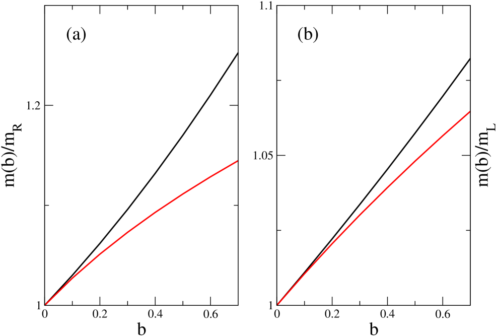
Figure 2: Magnetic field dependence of the particle’s mass in the lowest Landau level as a function of $B$ parametrized as $B=bT^{2}$ for (a) right-handed and (b) left-handed modes. Upper curves are the exact solutions and lower curves the analytical approximations.

The fact that for each mode there is only one non-vanishing solution to Eq. (77) means that only one projection of the spin relative to the direction of the external fields is able to propagate. This is precisely what one should expect for modes occupying the lowest possible energy level. The potential energy of a particle interacting with the external field is

$$U=-\vec{\mu}\cdot\vec{B}\propto-Y^{R,L}\vec{S}\cdot\vec{B}\,,$$ (78)

with $\vec{\mu}$, the particle’s magnetic moment and $\vec{S}$ the particle’s spin. Suppose the mode refers to a particle solution for a top-quark, then in Eq. (78), $Y^{R,L}>0$ . Thus, $U$ becomes a minimum for $\vec{S}$ and $\vec{B}$ parallel. Since the modes are chiral and also eigenfunctions of the helicity operator, left- (right)-handed particles can satisfy this condition only if $k_{3}<0$ $(k_{3}>0)$. This means that in the LLL, left- (right)-handed particles can only exist moving in the direction opposite (parallel) to the direction of the external field, with modes with the opposite value of $k_{3}$ being forbidden. For hole solutions the converse applies.

The dependence of the thermal mass on the magnetic field strength for the LLL modes can also be computed by considering the limit when $k_{3}\rightarrow 0$ in Eq. (77) which then becomes explicitly

$$k_{0}-\frac{m^{2}_{R,L}}{\sqrt{\frac{g^{\prime}}{2}Y^{R,L}B}}\ \frac{1}{2}\ln\left|\frac{k_{0}+\sqrt{\frac{g^{\prime}}{2}Y^{R,L}B}}{k_{0}-\sqrt{\frac{g^{\prime}}{2}Y^{R,L}B}}\right|=0\,.$$ (79)

In order to obtain analytical results, let us consider the limit in which $k_{0}\sim g^{\prime}T\gg\sqrt{g^{\prime}B}$. Then, we can use the Taylor expansion

$$\frac{1}{2}\ln\left(\frac{1+x}{1-x}\right)\simeq x+\frac{x^{3}}{3}\,,$$ (80)

into Eq. (79) and obtain

$$m_{R,L}(B) \equiv k_{0}^{R,L}(k_{3}=0)$$ (81)

$$= \frac{m_{R,L}}{\sqrt{2}}\left(1+\sqrt{1+\frac{2g^{\prime}Y^{R,L}B/3}{m^{2}_{R,L}}}\ \right)^{1/2}\!\!\!\!\!\!\!\!.$$

We thus see that the effect of the magnetic field is to increase the value of the thermal mass of the modes occupying the LLL. The increase however is different for left- and right-handed fields as the hypercharge for these modes is different. We also notice that in the limit when $B\rightarrow 0$, $m(B)_{R,L}\rightarrow m_{R,L}$.

Figure 2 shows the behavior of the solutions of Eq. (79) as functions of $B$ parametrized by $B=bT^{2}$. We have taken $g^{\prime}=0.344$, $g=0.637$ as corresponds to the values of these coupling constants at the EWPT epoch, as well as $g_{\phi}=1$, $Y_{R}=\frac{\mbox{\small}{4}}{\mbox{\small}{3}}$ and $Y_{L}=\frac{\mbox{\small}{1}}{\mbox{\small}{3}}$, as appropriate for top quarks. Also shown in the figure is the approximate analytical solution, Eq. (81). Notice that the difference between the exact and the approximate results grows with $b$ as is to be expected since the approximate solution, Eq. (81), is only valid for values of $b$ satisfying $g^{\prime}\gg b$.

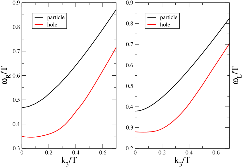
Figure 3: Dispersion relation as a function of the longitudinal momentum for right-handed (left panel) and left-handed (right panel) modes for $n=1$ and $b=0.1$. Upper curves are the particle solutions and lower curves the hole solutions. Notice that the presence of the magnetic field breaks the degeneracy for the mass of particle and hole solutions, pushing the former to larger and the latter to lower values, as compared to the thermal mass in the absence of a magnetic field, for the given value of $b$.

Figure 3 shows the dispersion relation for right- and left-handed modes in the Landau level with $n=1$. We have used a value for the magnetic field with $b=0.1$. Notice that the presence of the magnetic fields breaks the degeneracy in mass for particle and hole solutions. For the value of $b$ considered, the effect of the magnetic field is to increase the mass for particle and reduce it for hole solutions as compared to the value of the corresponding thermal mass in the absence of a magnetic field. The mass splitting is different however for right- and left-handed modes due to their different couplings to the external field.

Figure 4 shows the magnetic field dependence of the particle’s mass in the Landau level with n=10 as a function of $B$ parametrized as $B=bT^{2}$ for right- and left-handed modes. The mass splitting between particle and hole solutions is more important for left-handed modes for which the value of the hypercharge is smaller than the corresponding value for right-handed modes.

VI Summary and conclusions

In this work we have computed the dispersion relation for chiral fermions in the symmetric phase of the electroweak theory in the presence of a constant hypermagnetic field, at one loop level but all orders in $g^{\prime}B$. Working in the limit $T\gg\sqrt{g^{\prime}B}$, we have shown that left- and right-handed modes occupying the same Landau level, develop finite but different thermal masses due to the chiral nature of their coupling to the external field. In particular, in the LLL the thermal mass of the modes is increased with increasing field strength. For the rest of the levels with $n\neq 0$, the hypermagnetic field breaks the mass degeneracy for particle and hole solutions, however the mass splitting is different for left- and right-handed modes as their couplings to the external fields are different.

We have argued that, given the current bounds on the strength of primordial magnetic fields, the large temperature, weak field limit corresponds to the relevant scenario for the propagation of fermions prior and during the electroweak phase transition.

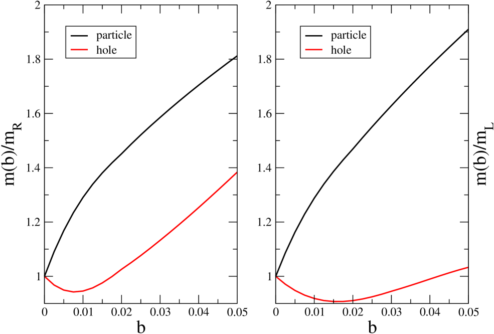
Figure 4: Magnetic field dependence of the particle’s mass in the n=10 Landau level as a function of $B$ parametrized as $B=bT^{2}$ for right-handed (left panel) and left-handed (right panel) modes. Upper curves are the particle and lower curves the hole solutions.

Though the numerical calculations are performed for top quarks, the results can also be applied to the case of any SM fermion species that can couple minimally to hypermagnetic fields prior to the EWPT through a non-vanishing hypercharge. Our work shows that the motion of such fermions is highly anisotropic since for any given Landau level, it is directed along the field lines. Neutrinos can prove to be another interesting case since at their decoupling, this anisotropic motion should be reflected in the properties of the cosmic background of relic neutrinos. Thus, if these relic neutrinos were to be detected and the anisotropy measured, this would provide a means of confirming the existence of primordial magnetic fields in the early universe. Another interesting consequence is the asymmetry that can be generated in decay processes of chiral fermions where particles with only one chirality are produced, such as beta decay. This is best illustrated for the case of the lowest Landau level where only one direction of motion is allowed for a given chirality of the decay products. The same asymmetry is present in higher Landau levels.

References

• (1) For reviews on the origin, evolution and some cosmological consequences of primordial magnetic fields see: K. Enqvist, Int. J. Mod. Phys. D7, 331 (1998); R. Maartens, Cosmological magnetic fields, International Conference on Gravitation and Cosmology, Pramana 55, 575 (2000) and references therein; D. Grasso and H.R. Rubinstein, Phys. Rep. 348, 163 (2001); L.M. Widrow, Rev. Mod. Phys. 74, 775 (2003).
• (2) See for example P.P. Kronberg, Rep. Prog. Phys. 57, 325 (1994); J.-L. Han and R. Wielebinski, Milestones in the Observations of Cosmic Magnetic Fields, astro-ph/0209090.
• (3) R. Beck, A. Brandenburg, D. Moss, A. Shukurov and D. Sokoloff, Annu. Rev. Astron. Astrophys. 34, 155 (1996).
• (4) J. A. Eilek and F. N. Owen, Ap. J. 567, 202 (2002).
• (5) T. E. Clarke, P. P. Kronberg and H. Böhringer, Ap. J. 547, L111 (2001).
• (6) M. Giovannini, Primordial Magnetic Fields, hep-ph/0208152.
• (7) J. Quashnock, A. Loeb and D.N. Spergel, Ap. J. 344, L49 (1989); B. Cheng and A.V. Olinto, Phys. Rev. D 50, 2421 (1994); G. Sigl, A.V. Olinto and K. Jedamzik, Phys. Rev. D 55, 4582 (1997).
• (8) G. Baym, D. Bödeker and L. McLerran, Phys. Rev. D 53, 662 (1996).
• (9) D. Boyanovsky, H. J. de Vega and M. Simionato, Large scale magnetogenesis from a non-equilibrium phase transition in the radiation dominated era, hep-ph/0211022.
• (10) A. Ayala, J. Besprosvany, G. Pallares and G. Piccinelli, Phys. Rev. D64, 123529 (2001); A. Ayala, G. Piccinelli and G. Pallares, Phys. Rev. D66, 103503 (2002).
• (11) A. Ayala and J. Besprosvany, Nucl. Phys. B 651, 211 (2003).
• (12) J. Cannellos, E.J. Ferrer, V. de la Incera, Phys. Lett. B 542, 123 (2002), E.J. Ferrer and V. de la Incera, Neutrinos under strong magnetic fields, hep-ph/0308017.
• (13) J.D. Barrow, P.G. Ferreira and J. Silk, Phys. Rev. Lett. 78, 3610 (1997).
• (14) J. Schwinger, Phys. Rev. 82. 664 (1951).
• (15) J.C. D’Olivo, J.F. Nieves and S. Sahu, Phys. Rev. D 67, 025018 (2003).
• (16) W. Dittrich and M. Reuter, Effective Lagrangians in Quantum Electrodynamics, Lecture Notes in Physics (Springer-Verlag, Berlin, 1985).
• (17) See for example, M. Le Bellac, Thermal Field Theory (Cambridge University Press, Cambridge, 1989).
• (18) P. Elmfors, D. Persson and B.-S. Skagerstam, Nucl. Phys. B 464, 153 (1996)
• (19) Similar expressions were first obtained by H.A. Weldon, Phys. Rev. D 26, 2789 (1982).