Full ${\cal O}(\alpha_{ew})$ electroweak corrections to $e^{+}e^{-}\rightarrow HHZ$

Abstract

We calculate the full ${\cal O}(\alpha_{ew})$ electroweak corrections to the Higgs pair production process $e^{+}e^{-}\rightarrow HHZ$ at an electron-positron linear collider in the standard model, and analyze the dependence of the Born cross section and the corrected cross section on the Higgs boson mass $m_{H}$ and the c.m. energy $\sqrt{s}$. To see the origin of some of the large corrections clearly, we calculate the QED and genuine weak corrections separately. The numerical results show that the corrections significantly suppress or enhance the Born cross section, depending on the values of $m_{H}$ and $\sqrt{s}$. For the c.m. energy $\sqrt{s}=500~{}{\rm GeV}$, which is the most favorable colliding energy for $HHZ$ production with intermediate Higgs boson mass, the relative correction decreases from $-5.3\%$ to $-11.5\%$ as $m_{H}$ increases from $100$ to $150~{}{\rm GeV}$. For the range of the c.m. energy where the cross section is relatively large, the genuine weak relative correction is small, less than $5\%$.

PACS: 12.15.Lk, 14.80.Bn, 14.70.Hp, 11.80.Fv
Keywords: electroweak correction, Higgs self-coupling, Higgs pair production

I Introduction

One of the most important goals of present and future colliders is to study the electroweak symmetry breaking mechanism and the origin of the masses of massive gauge bosons and fermions. As we know, within the Higgs mechanism [1] the electroweak gauge fields and fundamental matter fields (quarks and leptons) acquire their masses through the interaction with a scalar field (Higgs field) which has an nonzero vacuum expectation value (VEV). And the self-interaction of the Higgs field induces the spontaneous breaking of the electroweak ${\rm SU}(2)_{L}\otimes{\rm U}(1)_{Y}$ symmetry down to the electromegnetic ${\rm U}(1)_{EM}$ symmetry.

The present precise experimental data have shown an excellent agreement with the predictions of the standard model(SM) except for the Higgs sector [2]. These data strongly constrain the couplings of the gauge boson to fermions ($\lambda_{Zf\bar{f}}$ and $\lambda_{Wf\bar{f}^{\prime}}$), and the gauge self-couplings, but say little about the couplings of the Higgs boson to fermions ($\lambda_{Hf\bar{f}}$) and gauge bosons ($\lambda_{HZZ}$ and $\lambda_{HWW}$). Recent LEP2 experiment suggests that the Higgs boson has the mass with a lower bound of $114.4~{}{\rm GeV}$ and a upper bound of $193~{}{\rm GeV}$ at the $95\%$ confidence level [3] [4]. People believe that with the help of future high energy colliders, such as the CERN Large Hadron Collider (LHC) and Linear Colliders (LC’s), precise tests of the Higgs sector become possible. In the past few years, many theoretical works have been contributed to studying the Higgs boson productions and the properties of Higgs couplings at future high energy colliders [5] [6].

To reconstruct the Higgs potential and verify the Higgs mechanism experimentally, not only the Yukawa couplings and the couplings of the Higgs boson to gauge bosons should be measured, but also the Higgs self-couplings which include the trilinear coupling $\lambda_{HHH}$ and the quartic coupling $\lambda_{HHHH}$. These Higgs self-couplings can be probed directly only by multi-Higgs boson production. Due to the fact that the cross sections for three Higgs boson production processes are much smaller than those for Higgs boson pair production [7] [8], the quartic Higgs self-coupling remains elusive. Recently, the Higgs boson pair production processes have been widely considered, and the cross sections for these processes in the SM have been evaluated at linear colliders and hadron colliders. The phenomenology calculations show that it would be extremely difficult to measure the Higgs self-coupling $\lambda_{HHH}$ at the LHC [9], and $e^{+}e^{-}$ linear colliders, where the study of the $e^{+}e^{-}\rightarrow HHZ$ and $HH\nu\bar{\nu}$ can be performed with good accuracy, represent a possibly unique opportunity for performing the study of the trilinear Higgs self-coupling [7]. For the center of mass (c.m.) energy $\sqrt{s}$ from $500~{}{\rm GeV}$ up to about 1 TeV, the $HHZ$ production with intermediate Higgs boson mass is the most promising process among the various Higgs double-production processes, since its cross section is relatively large and all the final states can be identified without large missing momentum. When the c.m. energy $\sqrt{s}$ exceeds 1 TeV, the $e^{+}e^{-}\rightarrow HH\nu\bar{\nu}$ process becomes sizeable, and it is possible to measure the trilinear Higgs self-coupling $\lambda_{HHH}$ by using this process. Therefore, in the first stage of a LC ($\sqrt{s}<1~{}{\rm TeV}$), $e^{+}e^{-}\rightarrow HHZ$ is the most promising channel to measure the Higgs self-coupling $\lambda_{HHH}$.

Although the cross section for $e^{+}e^{-}\rightarrow HHZ$ with intermediate Higgs boson mass is only about $0.1\sim 0.2$ fb for $\sqrt{s}<1~{}{\rm TeV}$, the measurement of the Higgs self-coupling $\lambda_{HHH}$ through the process at $e^{+}e^{-}$ colliders can be significantly improved. For example, C. Castanier et al, conclude that a precision of about $10\%$ on the total cross section for $e^{+}e^{-}\rightarrow HHZ$ can be achieved leading to a relative error on $\lambda_{HHH}$ of $18\%$ with the help of high integrated luminosity $\int{\cal L}=2~{}{\rm ab}^{-1}$ after performing the detailed simulations of signal and background processes at the TESLA[10]. Other simulations demonstrate that the Higgs self-coupling $\lambda_{HHH}$ can be extracted more accurately by using a discriminating variable, namely the invariant mass of the HH system, and one can expect the high sensitivity of the triple Higgs self-coupling with an accuracy to $8\%$ and better in multi-TeV $e^{+}e^{-}$ collisions[11]. Therefore, to determine the Higgs self-couplings and reconstruct the Higgs potential, the theoretical prediction of the cross sections for $e^{+}e^{-}\rightarrow HHZ$ at a LC within per-cent accuracy is necessary. For this purpose, we investigate the $e^{+}e^{-}\rightarrow HHZ$ process at a LC in detail and present the calculation of the cross section for $e^{+}e^{-}\rightarrow HHZ$ with the full ${\cal O}(\alpha_{ew})$ electroweak corrections in the SM in this paper.

The paper is organized as follows: in section II we present the calculations of the Born cross section for $e^{+}e^{-}\rightarrow HHZ$ and the full ${\cal O}(\alpha_{ew})$ electroweak corrections to this process. The numerical results and discussions are presented in section III. In the last section, a short summary is given.

II Calculations

In this paper we adopt the ’t Hooft-Feynman gauge of the SM. At the tree level, there are six Feynman diagrams relevant to the process $e^{+}e^{-}\rightarrow HHZ$ ( shown in Fig.1). In Fig.1 only the second Feynman diagram (Fig.1(b)) contains a trilinear Higgs self-coupling vertex. In the SM the Higgs potential can be expressed as

$$V=\frac{m_{H}^{2}}{2}H^{2}+\frac{m_{H}^{2}}{2v}H^{3}+\frac{m_{H}^{2}}{8v^{2}}H^{4}$$ (2.1)

where $v=\left(\sqrt{2}G_{F}\right)^{-1/2}$. The trilinear Higgs self-coupling constant, $\lambda_{HHH}$, can be derived from this potential directly. By using the Higgs self-coupling constant $\lambda_{HHH}=3m_{H}^{2}/v$ and the relevant Feynman rules for gauge interactions, we can obtain the tree level amplitude ${\cal M}_{{\rm tree}}$ and the cross section $\sigma_{{\rm tree}}$ for $e^{+}e^{-}\rightarrow HHZ$.

Figure 1: The tree level Feynman diagrams for $e^{+}e^{-}\rightarrow HHZ$.

The ${\cal O}(\alpha_{ew})$ (one-loop level) virtual corrections to $e^{+}e^{-}\rightarrow HHZ$ can be expressed as

$$\sigma_{{\rm virtual}}=\sigma_{{\rm tree}}\delta_{{\rm virtual}}=\frac{(2\pi)^{4}}{2|\vec{p}_{1}|\sqrt{s}}\int{\rm d}\Phi_{3}\overline{\sum_{{\rm spin}}}{\rm Re}\left({\cal M}_{{\rm tree}}{\cal M}_{{\rm virtual}}^{\ast}\right),$$ (2.2)

where $\vec{p}_{1}$ is the c.m. momentum of the incoming positron, ${\rm d}\Phi_{3}$ is the three-body phase space element, and the bar over summation recalls averaging over initial spins [12]. ${\cal M}_{{\rm virtual}}$ is the amplitude of the virtual Feynman diagrams, including self-energy, vertex, box, pentagon and counterterm diagrams. All the Feynman diagrams and the relevant amplitudes are created by $FeynArts$ 3 [13], and the Feynman amplitudes are subsequently reduced by $FormCalc$ [14]. Due to the fact that the Yukawa coupling of Higgs/Goldstone to fermions is proportional to the fermion mass, we neglect the contributions of the Feynman diagrams which involve $H-e-\bar{e}$, $G^{0}-e-\bar{e}$, $G^{+}-e-\bar{\nu}_{e}$ or $G^{-}-\nu_{e}-\bar{e}$ vertex.

As we know, the contributions of the virtual diagrams contain both ultraviolet (UV) and infrared (IR) divergences, which can be regularized by extending the dimensions of spinor and spacetime manifolds to $D=4-2\epsilon$ [15] and giving the photon a fictitious mass $m_{\gamma}$, respectively. In this paper, we adopt the complete on-mass-shell (COMS) renormalization scheme [16] to fix all the renormalization constants. All the tensor coefficients of the one-loop integrals can be calculated by using the reduction formulae presented in Refs. [17] and [18]. As we expect, the UV divergence contributed by the loop diagrams can be cancelled by that contributed by the counterterm diagrams exactly, while the IR divergence still exists. Therefore, the ${\cal O}(\alpha_{ew}^{4})$ virtual cross section $\sigma_{{\rm virtual}}$ is independent of the UV regularization parameter $C_{{\rm UV}}=1/\epsilon-\gamma_{E}+{\rm log}4\pi$, but still a function of the IR regularization parameter $m_{\gamma}$.

In order to get an IR finite cross section for $e^{+}e^{-}\rightarrow HHZ$ up to the order of ${\cal O}(\alpha_{ew}^{4})$, we should consider the ${\cal O}(\alpha_{ew})$ corrections to $e^{+}e^{-}\rightarrow HHZ$ due to real photon emission. By using the general phase-space-slicing algorithm [19], the contributions to the photon emission process $e^{+}e^{-}\rightarrow HHZ\gamma$ are divided into a soft and a hard contribution,

$$\sigma_{{\rm real}}=\sigma_{{\rm soft}}+\sigma_{{\rm hard}}=\sigma_{{\rm tree}}\left(\delta_{{\rm soft}}+\delta_{{\rm hard}}\right),$$ (2.3)

where the “soft” and “hard” refer to the energy of the radiated photon. The energy $E_{\gamma}$ of the radiated photon in the c.m. frame is considered soft and hard if $E_{\gamma}\leq\Delta E$ and $E_{\gamma}>\Delta E$, respectively. Both $\sigma_{{\rm soft}}$ and $\sigma_{{\rm hard}}$ depend on the arbitrary soft cutoff $\Delta E/E_{b}$, where $E_{b}=\sqrt{s}/2$ is the electron beam energy in the c.m. frame, but the real cross section $\sigma_{{\rm real}}$ is cutoff independent. In our calculations the soft cutoff $\Delta E/E_{b}$ is set to be very small, therefore, the terms of order $\Delta E/E_{b}$ can be neglected and the soft contribution can be evaluated by using the soft photon approximation analytically [16] [20]

$${\rm d}\sigma_{{\rm soft}}=-{\rm d}\sigma_{{\rm tree}}\frac{\alpha_{ew}}{2\pi^{2}}\int_{|\vec{k}_{\gamma}|\leq\Delta E}\frac{{\rm d}^{3}k_{\gamma}}{2k^{0}_{\gamma}}\left(\frac{p_{1}}{p_{1}\cdot k_{\gamma}}-\frac{p_{2}}{p_{2}\cdot k_{\gamma}}\right)^{2}.$$ (2.4)

Here $k^{0}_{\gamma}=\sqrt{|\vec{k}_{\gamma}|^{2}+m_{\gamma}^{2}}$. $k_{\gamma}=(k^{0}_{\gamma},~{}\vec{k}_{\gamma})$ is the four momentum of the radiated photon, and $p_{1}$ and $p_{2}$ are the four momenta of $e^{+}$ and $e^{-}$, respectively. As shown in Eq. (2.4), the soft contribution has a IR singularity at $m_{\gamma}=0$. The IR divergence from the soft contribution cancels exactly that from the virtual corrections. Therefore, $\sigma_{{\rm virtual}+{\rm soft}}$, the sum of the ${\cal O}(\alpha_{ew}^{4})$ virtual and soft cross sections, is independent of the infinitesimal photon mass $m_{\gamma}$.

The hard contribution is UV and IR finite. It can be computed numerically by using standard Monte Carlo technique. In this paper, our computation of the hard contribution $\sigma_{{\rm hard}}$ is performed with the help of $CompHEP$ [21], which is a package for evaluation of tree level Feynman diagrams and integration over multi-particle phase space by using the adaptive multi-dimensional integration program Vegas [22].

Up to the order of ${\cal O}(\alpha_{ew}^{4})$, the corrected cross section for $e^{+}e^{-}\rightarrow HHZ$ is just the sum of the ${\cal O}(\alpha_{ew}^{3})$ Born cross section $\sigma_{{\rm tree}}$, the ${\cal O}(\alpha_{ew}^{4})$ virtual cross section $\sigma_{{\rm virtual}}$ and the ${\cal O}(\alpha_{ew}^{4})$ real cross section $\sigma_{{\rm real}}$,

$$\sigma_{{\rm tot}}=\sigma_{{\rm tree}}+\sigma_{{\rm virtual}}+\sigma_{{\rm real}}=\sigma_{{\rm tree}}\left(1+\delta_{{\rm tot}}\right),$$ (2.5)

where $\delta_{{\rm tot}}=\delta_{{\rm virtual}}+\delta_{{\rm soft}}+\delta_{{\rm hard}}$ is the full ${\cal O}(\alpha_{ew})$ electroweak relative correction. As we expect, the corrected cross section, $\sigma_{{\rm tot}}$, is independent of $C_{{\rm UV}}$ and $m_{\gamma}$, since it doesn’t contains any UV or IR singularity.

To discuss the origin of some of the large corrections, we need to calculate the photonic (QED) corrections and the genuine weak corrections separately. The QED corrections comprise two parts: the QED virtual corrections $\sigma_{{\rm virtual}}^{{\rm QED}}$ which contributed by the loop diagrams with virtual photon exchange in the loop and the corresponding parts of the counterterms, and the real corrections $\sigma_{{\rm real}}$. Therefore the QED relative correction $\delta_{{\rm E}}$ can be expressed as

$$\delta_{{\rm E}}=\delta_{{\rm virtual}}^{{\rm QED}}+\delta_{{\rm soft}}+\delta_{{\rm hard}},$$ (2.6)

where $\delta_{{\rm virtual}}^{{\rm QED}}=\sigma_{{\rm virtual}}^{{\rm QED}}/\sigma_{{\rm tree}}$, and the genuine weak relative correction $\delta_{{\rm W}}$ is defined as

$$\delta_{{\rm W}}=\delta_{{\rm tot}}-\delta_{{\rm E}}.$$ (2.7)

III Numerical results

For the numerical calculation we use the following SM input parameters [12],

$$m_{e}=0.510998902~{}{\rm MeV},~{}~{}~{}~{}~{}~{}m_{\mu}=105.658357~{}{\rm MeV},~{}~{}~{}~{}~{}~{}m_{\tau}=1.77699~{}{\rm GeV},~{}~{}~{}~{}~{}$$

$$m_{u}=66~{}{\rm MeV},~{}~{}~{}~{}~{}~{}~{}~{}~{}~{}~{}~{}~{}~{}~{}~{}~{}~{}~{}m_{c}=1.2~{}{\rm GeV},~{}~{}~{}~{}~{}~{}~{}~{}~{}~{}~{}~{}~{}~{}~{}~{}~{}m_{t}=174.3~{}{\rm GeV},~{}~{}~{}~{}~{}~{}~{}~{}$$

$$m_{d}=66~{}{\rm MeV},~{}~{}~{}~{}~{}~{}~{}~{}~{}~{}~{}~{}~{}~{}~{}~{}~{}~{}~{}m_{s}=150~{}{\rm MeV},~{}~{}~{}~{}~{}~{}~{}~{}~{}~{}~{}~{}~{}~{}~{}~{}m_{b}=4.3~{}{\rm GeV},~{}~{}~{}~{}~{}~{}~{}~{}~{}~{}~{}$$

$$m_{W}=80.423~{}{\rm GeV},~{}~{}~{}~{}~{}~{}~{}~{}~{}~{}~{}~{}~{}m_{Z}=91.1876~{}{\rm GeV},~{}~{}~{}~{}~{}~{}\alpha_{ew}^{-1}(0)=137.03599976.~{}~{}~{}~{}~{}$$ (3.1)

By using the relevant SM parameters listed above, we obtain

$$v=(\sqrt{2}G_{F})^{-1/2}=m_{W}\sin\theta_{W}/\sqrt{\pi\alpha_{ew}}=250.356~{}{\rm GeV}.$$ (3.2)

Besides these SM input parameters, six more input parameters should be given in the numerical calculation, which are the c.m. energy $\sqrt{s}$, the Higgs mass $m_{H}$, the mass parameter of dimensional regularization $Q$, the UV regularization parameter $C_{{\rm UV}}$, the IR regularization parameter $m_{\gamma}$ and the soft cutoff $\Delta E/E_{b}$. Since the corrected cross section $\sigma_{{\rm tot}}$ is independent of the mass parameter of dimensional regularization, we set $Q=1~{}{\rm GeV}$ in the numerical calculation.

In Table 1 we present some numerical results of the ${\cal O}(\alpha_{ew}^{4})$ cross section $\sigma_{{\rm virtual}+{\rm soft}}$ for $e^{+}e^{-}\rightarrow HHZ$, where the soft cutoff $\Delta E/E_{b}$ and the UV regularization parameter $C_{{\rm UV}}$ are set to be $\Delta E/E_{b}=10^{-3}$ and $C_{{\rm UV}}=0$, respectively. The middle two columns, labelled with I and II, are corresponding to the cases of $m_{\gamma}=10^{-20}~{}{\rm GeV}$ and $m_{\gamma}=1~{}{\rm GeV}$, respectively. Although the Monte Carlo statistical error of the cross section $\sigma_{{\rm virtual}+{\rm soft}}$ is the order of $10^{-3}$, we reserve the output numbers in columns I and II with 14 digits. By comparing the two columns of output numbers, we find that the results are stable over 8 digits when varying the fictitious photon mass $m_{\gamma}$ from $10^{-20}$ to $1~{}{\rm GeV}$. Therefore, we draw a conclusion that the ${\cal O}(\alpha_{ew}^{4})$ cross section $\sigma_{{\rm virtual}+{\rm soft}}$ is independent of $m_{\gamma}$ within the statistical error. The results with 4 (or 3) significant digits and the corresponding Monte Carlo integration errors are presented in the last column which is labelled with RES(ERR).

$$\begin{array}[]{c@{\quad}c@{\quad}c}\hline\cr\sqrt{s}~{}[{\rm GeV}]&m_{H}~{}[{\rm GeV}]&\begin{array}[]{c}\sigma_{{\rm virtual}+{\rm soft}}~{}[{\rm fb}]\\ ~{}~{}~{}~{}~{}~{}~{}~{}~{}~{}~{}~{}~{}~{}{\rm I}~{}~{}~{}~{}~{}~{}~{}~{}~{}~{}~{}~{}~{}~{}~{}~{}~{}~{}~{}~{}~{}~{}~{}~{}~{}~{}~{}~{}~{}~{}{\rm II}~{}~{}~{}~{}~{}~{}~{}~{}~{}~{}~{}~{}~{}~{}~{}~{}~{}{\rm RES}({\rm ERR})\end{array}\\ \hline\cr 500&115&-0.13108006089013~{}~{}~{}~{}~{}-0.13108006072333~{}~{}~{}~{}~{}-0.1311(2)\\ &150&-0.05089427858862~{}~{}~{}~{}~{}-0.05089427861858~{}~{}~{}~{}~{}-0.0509(1)\\ \hline\cr 800&115&-0.10810404820086~{}~{}~{}~{}~{}-0.10810404820051~{}~{}~{}~{}~{}-0.1081(3)\\ &150&-0.08643256423041~{}~{}~{}~{}~{}-0.08643256423012~{}~{}~{}~{}~{}-0.0864(2)\\ \hline\cr 1000&115&-0.09123978783411~{}~{}~{}~{}~{}-0.09123978977518~{}~{}~{}~{}~{}-0.0912(3)\\ &150&-0.08051191441546~{}~{}~{}~{}~{}-0.08051191441530~{}~{}~{}~{}~{}-0.0805(2)\\ \hline\cr 2000&115&-0.04961299068878~{}~{}~{}~{}~{}-0.04961299068876~{}~{}~{}~{}~{}-0.0496(2)\\ &150&-0.04848771307528~{}~{}~{}~{}~{}-0.04848771307526~{}~{}~{}~{}~{}-0.0485(2)\\ \hline\cr\end{array}$$

Table 1: The ${\cal O}(\alpha_{ew}^{4})$ cross section $\sigma_{{\rm virtual}+{\rm soft}}$ for $e^{+}e^{-}\rightarrow HHZ$ process for various Higgs boson mass (115 GeV and 150 GeV) and c.m. energy values (500 GeV, 800 GeV, 1000 GeV and 2000 GeV).

Analogously, the UV finiteness of $\sigma_{{\rm virtual}}$ can also be checked numerically. We find that the numerical results of $\sigma_{{\rm virtual}}$ are stable over 7 digits when varying the UV regularization parameter $C_{{\rm UV}}$ from 0 to $10^{5}$ for various $\sqrt{s}$ and $m_{H}$. For simplicity, we do not present these numerical results in this section.

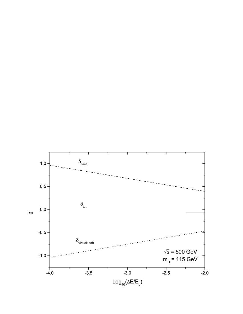
Figure 2: The ${\cal O}(\alpha_{ew})$ relative correction to $e^{+}e^{-}\rightarrow HHZ$ as a function of the soft cutoff $\Delta E/E_{b}$.

Figure 3: The dependence of the corrected cross section for $e^{+}e^{-}\rightarrow HHZ$ on the soft cutoff $\Delta E/E_{b}$.

In Fig.2 we present the ${\cal O}(\alpha_{ew})$ relative correction to $e^{+}e^{-}\rightarrow HHZ$ as a function of the soft cutoff $\Delta E/E_{b}$, assuming $m_{H}=115~{}{\rm GeV}$ and $\sqrt{s}=500~{}{\rm GeV}$. As shown in this figure, both $\delta_{{\rm virtual}+{\rm soft}}$ ($=\delta_{{\rm virtual}}+\delta_{{\rm soft}}$) and $\delta_{{\rm hard}}$ depend on the soft cutoff $\Delta E/E_{b}$, but the full ${\cal O}(\alpha_{ew})$ electroweak relative correction $\delta_{{\rm tot}}$ is cutoff independent. To show the cutoff independence more clearly, we present $\sigma_{{\rm tot}}$, the corrected cross section for $e^{+}e^{-}\rightarrow HHZ$ which includes the full ${\cal O}(\alpha_{ew})$ electroweak corrections, with the statistical errors from the Monte Carlo integration in Fig.3. As shown in Fig.3, a clear plateau is reached for $\Delta E/E_{b}$ in the range $10^{-4}-10^{-2}$ and the corrected cross section $\sigma_{{\rm tot}}$ is obviously independent of $\Delta E/E_{b}$.

Until now, we have checked the $m_{\gamma}$, $C_{{\rm UV}}$ and $\Delta E/E_{b}$ independence of the full ${\cal O}(\alpha_{ew})$ electroweak corrections to $e^{+}e^{-}\rightarrow HHZ$. In the following calculation, $m_{\gamma}$, $C_{{\rm UV}}$ and $\Delta E/E_{b}$ are fixed to be $10^{-2}~{}{\rm GeV}$, 0 and $10^{-3}$, respectively.

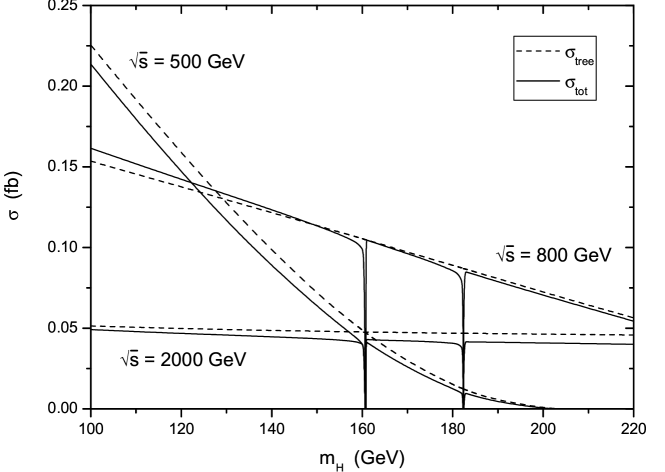
Figure 4: The Born cross section and the corrected cross section for $e^{+}e^{-}\rightarrow HHZ$ as functions of the Higgs boson mass.

Figure 5: The full ${\cal O}(\alpha_{ew})$ electroweak relative correction to $e^{+}e^{-}\rightarrow HHZ$ as a function of the Higgs boson mass.

In Fig.4 we present the Born cross section $\sigma_{{\rm tree}}$ and the corrected cross section $\sigma_{{\rm tot}}$ for $e^{+}e^{-}\rightarrow HHZ$ as functions of the Higgs boson mass $m_{H}$ for $\sqrt{s}=500$, $800$ and $2000~{}{\rm GeV}$, respectively. As shown in this figure, each solid curve has two spikes at the vicinities of $m_{H}=2m_{W}$ and $m_{H}=2m_{Z}$, which just reflect the resonance effects at $m_{H}=2m_{W}$ and $m_{H}=2m_{Z}$, respectively. For $\sqrt{s}=2000~{}{\rm GeV}$, both $\sigma_{{\rm tree}}$ and $\sigma_{{\rm tot}}$ are insensitive to $m_{H}$, decrease very slowly as the increment of $m_{H}$ from $100$ to $220~{}{\rm GeV}$. In contrast to the case of $\sqrt{s}=2000~{}{\rm GeV}$, the cross sections are sensitive to $m_{H}$ when $\sqrt{s}=500~{}{\rm GeV}$. They decrease rapidly to zero as $m_{H}$ increases to about $204~{}{\rm GeV}$.

To describe the full ${\cal O}(\alpha_{ew})$ electroweak corrections to the Born cross section for $e^{+}e^{-}\rightarrow HHZ$ quantitatively, we plot the full ${\cal O}(\alpha_{ew})$ relative correction $\delta_{{\rm tot}}$, defined as $\delta_{{\rm tot}}=(\sigma_{{\rm tot}}-\sigma_{{\rm tree}})/\sigma_{{\rm tree}}$, as a function of $m_{H}$ in Fig.5. For $\sqrt{s}=500~{}{\rm GeV}$, which is the most favorable c.m. energy for $e^{+}e^{-}\rightarrow HHZ$ with intermediate Higgs boson mass, the relative correction is negative in the range of $100~{}{\rm GeV}<m_{H}<204~{}{\rm GeV}$. It decreases from $-5.3\%$ to $-11.50\%$ as $m_{H}$ increases from 100 to 150 GeV. Since the cross section near threshold is very small, the large relative correction in this region is phenomenologically insignificant. For $\sqrt{s}=2000~{}{\rm GeV}$, the relative correction is also negative in the range of $100~{}{\rm GeV}<m_{H}<220~{}{\rm GeV}$. It decreases from $-4.6\%$ to $-12.5\%$ as the increment of $m_{H}$ from $100$ to $220{\rm GeV}$. For $\sqrt{s}=800~{}{\rm GeV}$, the relative correction is positive when $m_{H}<150~{}{\rm GeV}$. It varies from $5.2\%$ to $-3.7\%$ as $m_{H}$ running from 100 to 220 GeV. The numerical results of $\sigma_{{\rm tree}}$, $\sigma_{{\rm tot}}$ and $\delta_{{\rm tot}}$ for some typical values of $m_{H}$ and $\sqrt{s}$ are presented in Table 2.

$$\begin{array}[]{c@{\quad}c@{\quad}l@{\quad}l@{\quad}l}\hline\cr\sqrt{s}~{}[{\rm GeV}]&m_{H}~{}[{\rm GeV}]&\sigma_{{\rm tree}}~{}[{\rm fb}]&\sigma_{{\rm tot}}~{}[{\rm fb}]&\delta_{{\rm tot}}~{}[\%]\\ \hline\cr&115&0.17493(2)&0.1629(2)&-6.9(1)\\ 500&150&0.071834(6)&0.06357(6)&-11.50(7)\\ &200&0.49611(3)\cdot 10^{-3}&0.3329(2)\cdot 10^{-3}&-32.90(4)\\ \hline\cr&115&0.17428(2)&0.1740(3)&-0.2(1)\\ 600&150&0.10840(1)&0.1041(1)&-4.0(1)\\ &200&0.031802(3)&0.02935(2)&-7.71(7)\\ \hline\cr&115&0.15868(3)&0.1632(3)&\phantom{-}2.8(2)\\ 700&150&0.11665(2)&0.1155(2)&-1.0(1)\\ &200&0.058846(7)&0.05665(7)&-3.7(1)\\ \hline\cr&115&0.14156(3)&0.1471(3)&\phantom{-}3.9(2)\\ 800&150&0.11363(2)&0.1135(2)&-0.1(2)\\ &200&0.07246(1)&0.0705(1)&-2.7(1)\\ \hline\cr&115&0.11293(2)&0.1168(3)&\phantom{-}3.4(3)\\ 1000&150&0.09890(2)&0.0983(3)&-0.6(2)\\ &200&0.07790(1)&0.0753(2)&-3.3(2)\\ \hline\cr&115&0.07119(2)&0.0704(3)&-1.1(4)\\ 1500&150&0.06684(2)&0.0634(2)&-5.1(3)\\ &200&0.06165(1)&0.0569(2)&-7.7(3)\\ \hline\cr&115&0.05021(1)&0.0473(2)&-5.8(4)\\ 2000&150&0.04812(1)&0.0435(2)&-9.6(4)\\ &200&0.04630(1)&0.0408(2)&-11.9(4)\\ \hline\cr\end{array}$$

Table 2: The Born cross section $\sigma_{{\rm tree}}$, the corrected cross section $\sigma_{{\rm tot}}$ and the full ${\cal O}(\alpha_{ew})$ electroweak relative correction $\delta_{{\rm tot}}$ for various Higgs boson mass and c.m. energy values.

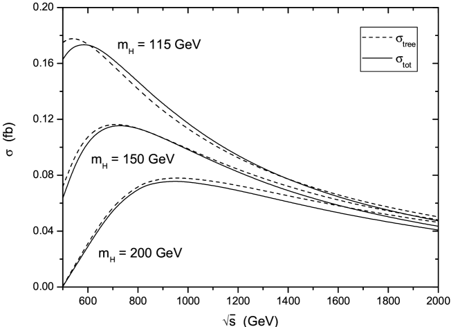
Figure 6: The Born cross section and the corrected cross section for $e^{+}e^{-}\rightarrow HHZ$ as functions of the c.m. energy.

Figure 7: The full ${\cal O}(\alpha_{ew})$ electroweak relative correction to $e^{+}e^{-}\rightarrow HHZ$ as a function of the c.m. energy.

In Fig.6 we depict the Born cross section $\sigma_{{\rm tree}}$ and the corrected cross section $\sigma_{{\rm tot}}$ for $e^{+}e^{-}\rightarrow HHZ$ as functions of the c.m. energy $\sqrt{s}$ for $m_{H}=115$, 150 and 200 GeV, respectively. The c.m. energy varies in the range $500~{}{\rm GeV}<\sqrt{s}<2000~{}{\rm GeV}$, which is accessible at future linear colliders, such as TESLA [23], NLC [24], JLC [25] and CERN CLIC [26]. From this figure we find that both the Born cross section $\sigma_{{\rm tree}}$ and the corrected cross section $\sigma_{{\rm tot}}$ increase firstly, reach their maximal values, and then decrease with the increment of $\sqrt{s}$. For $m_{H}=115~{}{\rm GeV}$, $\sigma_{{\rm tree}}$ and $\sigma_{{\rm tot}}$ reach their maximal values of about 0.178 and 0.174 fb at $\sqrt{s}\sim 550~{}{\rm GeV}$ and $\sqrt{s}\sim 600~{}{\rm GeV}$, respectively. For $m_{H}=150~{}{\rm GeV}$ $\sigma_{{\rm tree}}$ and $\sigma_{{\rm tot}}$ reach the maximums of about 0.117 and 0.116 fb at $\sqrt{s}\sim 700~{}{\rm GeV}$, and for $m_{H}=200~{}{\rm GeV}$ they reach about 0.078 and 0.076 fb at $\sqrt{s}\sim 950~{}{\rm GeV}$, respectively.

The dependence of the full ${\cal O}(\alpha_{ew})$ electroweak relative correction to $e^{+}e^{-}\rightarrow HHZ$ on the c.m. energy $\sqrt{s}$ is displayed in Fig.7. As shown in this figure, the full ${\cal O}(\alpha_{ew})$ electroweak corrections suppress the Born cross section in the c.m. energy range of $500~{}{\rm GeV}<\sqrt{s}<2000~{}{\rm GeV}$ for $m_{H}=150$ and 200 GeV, while enhance the Born cross section in the c.m. energy range of $610~{}{\rm GeV}<\sqrt{s}<1360~{}{\rm GeV}$ for $m_{H}=115~{}{\rm GeV}$. The relative corrections can reach about $-6.9\%$ and $-11.5\%$ at $\sqrt{s}=500~{}{\rm GeV}$ for $m_{H}=115$ and 150 GeV respectively. For $m_{H}=200~{}{\rm GeV}$, the relative correction is large and can exceed $-10\%$. It ranges from $-2.7\%$ to $-11.9\%$ as $\sqrt{s}$ varying in the range of $800~{}{\rm GeV}<\sqrt{s}<2000~{}{\rm GeV}$. We can see that in some parameter space the electroweak relative corrections are only few percent and might be below the achievable experimental accuracy.

Figure 8: The dependence of the QED relative correction $\delta_{E}$ and the genuine weak relative correction $\delta_{W}$ to $e^{+}e^{-}\rightarrow HHZ$ on the Higgs boson mass.

In Fig.8 we present the dependence of the QED relative correction $\delta_{\rm E}$ and the genuine weak relative correction $\delta_{\rm W}$ to $e^{+}e^{-}\rightarrow HHZ$ on the Higgs boson mass separately. From this figure we find that at threshold the genuine weak relative correction is a striking contrast to the QED relative correction, and the contribution of the ${\cal O}(\alpha_{ew})$ electroweak correction is overwhelmingly dominanted by the QED correction. For $\sqrt{s}=500~{}{\rm GeV}$, the genuine weak relative correction strongly depends on the Higgs boson mass. It increases from $-1.20\%$ to $4.56\%$ as $m_{H}$ increases from 100 to 150 GeV. For $\sqrt{s}=2000$ GeV, the genuine weak relative correction is insensitive to the Higgs boson mass. It is about $-15\%\sim-17\%$ for $m_{H}$ in the range of $100~{}{\rm GeV}<m_{H}<220~{}{\rm GeV}$.

The $\sqrt{s}$ dependence of the QED relative correction $\delta_{\rm E}$ and genuine weak relative correction $\delta_{\rm W}$ to $e^{+}e^{-}\rightarrow HHZ$ are displayed in Fig.9. Together with Fig.6 we can see from this figure that for the range of $\sqrt{s}$ where the cross section is relatively large, the QED relative correction is not too large and the genuine weak relative correction is less than $5\%$. For $\sqrt{s}>1000~{}{\rm GeV}$, the Higgs mass dependence of the genuine weak relative correction is small. As $\sqrt{s}$ increases to $2000~{}{\rm GeV}$, the genuine weak relative correction can reach about $-15\%\sim-18\%$ for $m_{H}$ in the range of $115~{}{\rm GeV}<m_{H}<200~{}{\rm GeV}$.

Figure 9: The dependence of the QED relative correction and the genuine weak relative correction to $e^{+}e^{-}\rightarrow HHZ$ on the c.m. energy.

IV Summary

In this paper we calculate the full ${\cal O}(\alpha_{ew})$ electroweak corrections to $e^{+}e^{-}\rightarrow HHZ$ at a LC in the SM, and analyze the dependence of the Born cross section, the corrected cross section including full ${\cal O}(\alpha_{ew})$ electroweak corrections and the relative correction on the $m_{H}$ and $\sqrt{s}$. To see the origin of some of the large corrections clearly, we calculate the QED and genuine weak corrections separately. From the numerical results we find that the full ${\cal O}(\alpha_{ew})$ electroweak corrections significantly suppress or enhance the Born cross section, depending on the Higgs boson mass and the c.m. energy of a LC. Both the Born cross section and the corrected cross section are insensitive to the Higgs boson mass in the range of $100~{}{\rm GeV}<m_{H}<220~{}{\rm GeV}$ for $\sqrt{s}=2000~{}{\rm GeV}$, but strongly related to the Higgs boson mass in the range of $100~{}{\rm GeV}<m_{H}<204~{}{\rm GeV}$ for $\sqrt{s}=500~{}{\rm GeV}$. With our chosen $\sqrt{s}-m_{H}$ parameter space in this paper, the relative corrections are a few percent generally, and can exceed $-10\%$ when $\sqrt{s}\sim 500~{}{\rm GeV}$ and $m_{H}\sim 150~{}{\rm GeV}$. Therefore, the full ${\cal O}(\alpha_{ew})$ electroweak corrections should be taken into account in the precise experiment analysis. We should also mention that in some parameter space, where the cross section is sizeable, the total relative corrections are only few percent and thus probably might be below the achievable experimental accuracy.

Note Added: As we were amending this manuscript, we became aware of a similar paper by G. Belanger, et al.,[27]. They presented a numerical comparison in Table 3 of Ref.[27].

Acknowledgments: This work was supported in part by the National Natural Science Foundation of China and a grant from the University of Science and Technology of China.

Figure Captions

Figure 1 The tree level Feynman diagrams for $e^{+}e^{-}\rightarrow HHZ$.

Figure 2 The ${\cal O}(\alpha_{ew})$ relative correction to $e^{+}e^{-}\rightarrow HHZ$ as a function of the soft cutoff $\Delta E/E_{b}$.

Figure 3 The dependence of the corrected cross section for $e^{+}e^{-}\rightarrow HHZ$ on the soft cutoff $\Delta E/E_{b}$.

Figure 4 The Born cross section and the corrected cross section for $e^{+}e^{-}\rightarrow HHZ$ as functions of the Higgs boson mass.

Figure 5 The full ${\cal O}(\alpha_{ew})$ electroweak relative correction to $e^{+}e^{-}\rightarrow HHZ$ as a function of the Higgs boson mass.

Figure 6 The Born cross section and the corrected cross section for $e^{+}e^{-}\rightarrow HHZ$ as functions of the c.m. energy.

Figure 7 The full ${\cal O}(\alpha_{ew})$ electroweak relative correction to $e^{+}e^{-}\rightarrow HHZ$ as a function of the c.m. energy.

Figure 8 The dependence of the QED relative correction and the genuine weak relative correction to $e^{+}e^{-}\rightarrow HHZ$ on the Higgs boson mass.

Figure 9 The dependence of the QED relative correction and the genuine weak relative correction to $e^{+}e^{-}\rightarrow HHZ$ on the c.m. energy.

Table 1 The ${\cal O}(\alpha_{ew}^{4})$ cross section $\sigma_{{\rm virtual+soft}}$ for $e^{+}e^{-}\rightarrow HHZ$ process for various Higgs boson mass (115 GeV and 150 GeV) and c.m. energy values (500 GeV, 800 GeV, 1000 GeV and 2000 GeV).

Table 2 The Born cross section $\sigma_{{\rm tree}}$, the corrected cross section $\sigma_{{\rm tot}}$ and the full ${\cal O}(\alpha_{ew})$ electroweak relative correction $\delta_{{\rm tot}}$ for various Higgs boson mass and c.m. energy values.

References

• [1] P. W. Higgs, Phys. Lett. 12, 132 (1964); and Phys. Rev. 145, 1156 (1996); F. Englert and R. Brout, Phys. Rev. Lett. 13, 321 (1964); G. S. Guralnik, C. R. Hagen and T. W. Kibble, Phys. Rev. Lett. 13, 585 (1964).
• [2] The LEP Collaborations, LEPEWWG/TGC/2002-03 (Sept. 2001); β€œThe QCD/SM Working Group: Summary Report”, hep-ph/0204316.
• [3] ALEPH, DELPHI, L3 and OPAL, (The LEP working group for Higgs boson searches), Contributed paper for ICHEP’02, Amsterdam, July 2002, ALEPH 2002-024, CONF 2002-013, DLPHI 2002-088-CONF-621, L3 Note 2766, OPAL Technical Note TN721, LHWG Note/2002-01; P. A. McNamara and S. L. Wu, Rept. Prog. Phys. 65, 465 (2002).
• [4] M. W. Β GrΓΌnewald, Nucl. Phys. Proc. Suppl. 117, 280 (2003); ALEPH, DELPHI, L3 and OPAL, the LEP Higgs working group, hep-ex/0107029; U. Schwickerath, hep-ph/0205126.
• [5] M. Baillargeon, F. Boudjema, F. Cuypers, E. Gabrielli and B. Mele, Nucl. Phys. B424, 343 (1994); A. Ballestrero, E. Maina and S. Moretti, Phys. Lett. B335, 460 (1994); and Phys. Lett. B333, 434 (1994); S. Moretti, Z. Phys. C71, 267 (1996); W. Kilian, M. KrΓ€mer and P. M. Zerwas, Phys. Lett. B373, 135 (1996).
• [6] H. J. Lu and J. Milana, Phys. Rev. D51, 6107 (1995); A. Djouadi and P. Gambino, Phys. Rev. Lett. 73, 2528 (1994); M. Spira, A. Djouadi, D. Graudenz and P. M. Zerwas, Nucl. Phys. B453, 17 (1995); R. P. Kauffman, S. V. Desai and D. Risal, Phys. Rev. D55 4005 (1997); Erratum-ibid. D58, 119901 (1998); R. Harlander and W. Kilgore, Int. J. Mod. Phys. A16S1A, 305 (2001).
• [7] A. Djouadi, W. Kilian, M. Muhlleitner and P. M. Zerwas, Eur. Phys. J. C10, 45 (1999); M. Battaglia, E. Boos and W. M. Yao, hep-ph/0111276; A. Djouadi, W. Kilian, M. Muhlleitner and P. M. Zerwas, hep-ph/0001169.
• [8] D. A. Dicus, C. Kao and S. S. Willenbrock, Phys. Lett. B203, 457 (1988); E. W. Glover and J. J. van der Bij, Nucl. Phys. B309, 282 (1988); T. Plehn, M. Spira and P. M. Zerwas, Nucl. Phys. B479, 46 (1996); Erratum-ibid. B531, 655 (1998).
• [9] U. Baur, T. Plehn and D. Rainwater, Phys. Rev. Lett. 89, 151801 (2002).
• [10] C. Castanier, P. Gay, P. Lutz and J. Orloff, hep-ex/0101028.
• [11] M. Battaglia, E. Boos and W. Yao, hep-ph/0111276; Y. Yashui, $et$ $al$, hep-ph/0211047.
• [12] K. Hagiwara, $et$ $al$., Phys. Rev. D66, 010001 (2002).
• [13] T. Hahn, Comput. Phys. Commun. 140, 418 (2001).
• [14] T. Hahn, $FormCalc$ $3.2$ U​s​e​r′​sπ‘ˆπ‘ π‘’superscriptπ‘Ÿβ€²π‘ User^{\prime}s $Guide$, http://www.feynarts.de/formcalc.
• [15] G. ’t Hooft and M. Veltman, Nucl. Phys. B44, 189 (1972).
• [16] A. Denner, Fortschr. Phys. 41, 307 (1993).
• [17] G. Passarino and M. Veltman, Nucl. Phys. B160, 151 (1979).
• [18] A. Denner and S. Dittmaier, Nucl. Phys. B658, 175 (2003).
• [19] W. T. Giele and E. W. Glover, Phys. Rev. D46, 1980 (1992); W. T. Giele, E. W. Glover and D. A. Kosower, Nucl. Phys. B403, 633 (1993); S. Keller and E. Laenen, Phys. Rev. D59, 114004 (1999).
• [20] G. ’t Hooft and Veltman, Nucl. Phys. B153, 365 (1979).
• [21] A. Pukhov, $et$ $al$., hep-ph/9908288.
• [22] G. P. Lepage, J. Comput. Phys. 27, 192 (1978) and CLNS-80/447.
• [23] β€œTELSA, The Superconducting Electron Positron Linear Collider with an Integrated X-Ray Laser Laboratory: Technical Design Report”, DESY-2001-011, ECFA-2001-209, TESLA-2001-23, TESLA-FEL-2001-05, (March, 2001).
• [24] T. Raubenheimer, β€œNLC”, a linear collider status report given at the Linear Collider Workshop 2000.
• [25] N. Akasaka $et$ $al$., β€œJLC Design Study”,KEK-REPORT-97-1.
• [26] G. Guignard (editor), β€œA 3 TeV $e^{+}e^{-}$ Linear Collider Based on CLIC Technology”, CERN-2000-008.
• [27] G. Belanger $et$ $al$., ”Full ${\cal O}$($\alpha$) electroweak corrections to double Higgs-strahlung at the linear collider”, LAPTH-994, KEK-CP-142, arXiv:hep-ph/0309010.