Chiral dynamics and the growth of the nucleon’s gluonic transverse size at small $x$

Abstract

We study the distribution of gluons in transverse space in the nucleon at moderately small $x$ ($\sim 10^{-2}$). At large transverse distances (impact parameters) the gluon density is generated by the “pion cloud” of the nucleon, and can be calculated in terms of the gluon density in the pion. We investigate the large–distance behavior in two different approaches to chiral dynamics: i) phenomenological soft–pion exchange, ii) the large–$N_{c}$ picture of the nucleon as a classical soliton of the pion field, which corresponds to degenerate $N$ and $\Delta$ states. The large–distance contributions from the “pion cloud” cause a $\sim 20\%$ increase in the overall transverse size of the nucleon if $x$ drops significantly below $M_{\pi}/M_{N}$. This is in qualitative agreement with the observed increase of the slope of the $t$–dependence of the $J/\psi$ photoproduction cross section at HERA compared to fixed–target energies. We argue that the glue in the pion cloud could be probed directly in hard electroproduction processes accompanied by “pion knockout”, $\gamma^{\ast}+N\;\rightarrow\;\gamma\;(\mbox{or}\;\;\rho,\,J/\psi)\;+\pi+N^{\prime}$, where the transverse momentum of the emitted pion is large while that of the outgoing nucleon is restricted to values of order $M_{\pi}$.

I Introduction

Hard scattering processes induced by (real or virtual) photons are an important source of information about the structure of the nucleon. The parton model description of such processes distinguishes a “longitudinal” direction, defined by the 3–momentum of the incoming photon, and the “transverse” plane perpendicular to it. The structure functions of inclusive deep–inelastic scattering are proportional to the parton densities, describing the distribution of partons with respect to longitudinal momentum of the parent nucleon; they do not carry any information about the distribution of partons in the transverse plane. In this sense, inclusive deep–inelastic scattering provides us with a 1–dimensional image of the nucleon. Much more detailed information can be obtained from exclusive processes, in which one measures amplitudes with a non-zero momentum transfer between the initial and final nucleon, $\Delta=p^{\prime}-p\neq 0$, with $t\equiv\Delta^{2}<0$. These include hard electroproduction processes such as deeply–virtual Compton scattering and meson production, or diffractive photoproduction of heavy quarkonia ($J/\psi,\Upsilon$), which probes the gluon distribution in the nucleon. Such measurements can give information also about the spatial distribution of partons in the transverse plane, thus providing us with a 3–dimensional image of the nucleon.

A precise formulation of the notion of a spatial distribution of partons in the transverse plane is possible within the formalism of generalized parton distributions (GPD’s), which parametrize the non-forward matrix elements ($p^{\prime}\neq p$) of twist–2 QCD light–ray operators between nucleon states Muller:1998fv ; Ji:1997nm ; Radyushkin:1997ki ; Collins:1996fb . Of particular interest is the “diagonal” limit of zero longitudinal component of the momentum transfer, $\Delta^{+}=0$. The GPD’s in this case depend (in addition to the partonic variable, $x$) only on the transverse component of the momentum transfer, ${\bf\Delta}_{\perp}$, with $-{\bf\Delta}_{\perp}^{2}=t$, and the nucleon helicity–conserving ones reduce to the usual polarized and unpolarized parton densities in the limit $t\rightarrow 0$ (for this reason the $\Delta^{+}=0$ GPD’s are also referred to as “non-forward parton densities” Radyushkin:1998rt ). The Fourier transform of these functions with respect to ${\bf\Delta}_{\perp}$ then defines functions of a 2–dimensional coordinate variable, ${\bf b}$, which can be interpreted as the spatial distributions of partons with longitudinal momentum fraction $x$ in the transverse plane (“impact parameter–dependent parton distributions”) Burkardt:2002hr . The integral of these ${\bf b}$–dependent distributions reproduce the total densities of partons for given $x$, and they can be shown to satisfy positivity conditions locally in ${\bf b}$ Pobylitsa:2002iu . This “mixed” momentum and coordinate representation provides a vivid 3–dimensional (more precisely, $1+2$–dimensional) picture of the partonic structure of the nucleon, which naturally lends itself to the visualization of polarization effects, including orbital angular momentum Burkardt:2002hr . On the phenomenological side, it has been speculated that this representation could provide a simple explanation of the transverse single spin asymmetries observed in semi-inclusive deep–inelastic scattering Burkardt:2002ks .

It should be noted that the “diagonal” GPD’s ($\Delta^{+}=0$) are not directly observable, since hard exclusive processes generally have skewed kinematics. However, in a number of important cases the kinematics is effectively not far from the diagonal case. In particular, this is the case for $J/\psi$ photoproduction, which probes the generalized gluon distribution in the nucleon; the ratio of the longitudinal momentum fractions of the two gluons is of the order $x_{1}/x_{2}\sim 2$ Frankfurt:1997fj . Furthermore, for $\Upsilon$ production Martin:1999rn , and generally for electroproduction at large $Q^{2}$ and sufficiently small $x$ Frankfurt:1998yf , the gluon GPD’s are dominated by evolution down from significantly larger values of $x_{1}$ and $x_{2}$. Since the difference $x_{1}-x_{2}$ is not changed by the evolution, this implies that one is actually probing the $t$–dependence of the nearly diagonal distributions at larger $x_{1}$ and $x_{2}$ (the $t$–dependence is not affected by the evolution).

An interesting aspect of the impact parameter representation of parton distributions, which has been less emphasized so far, is that it provides a useful new framework for developing dynamical models for (generalized) parton distributions. The possibility to separate contributions from different transverse distance scales allows one to introduce the notion of a “size” of the nucleon, well–known from elastic form factors (charge radii), in the discussion of generalized parton distributions. Furthermore, one can incorporate the fundamental fact that the long–distance behavior of strong interactions is governed by chiral dynamics. Thus, one would expect that, in a certain range of $x$, the parton distributions at transverse distances of order $1/M_{\pi}$ can be attributed to the “pion cloud” of the nucleon, and can be computed from first principles in terms of the known parton distributions in the pion. This would provide model–independent constraints for the distributions of partons in the transverse plane. Moreover, the partons in the pion cloud may lead directly to observable effects in hard processes sensitive to large transverse distances.

In this paper we study the impact parameter dependence of the nucleon’s gluon density from a phenomenological perspective. We concentrate on the region of moderately small $x$ ($\sim 10^{-2}$), for which the $t$–dependence of the gluon GPD (the so-called “two–gluon form factor” of the nucleon) has been extracted from a number of electro–/photoproduction experiments, see Ref.Frankfurt:2002ka for a compilation. The investigation consists of three parts. First, we derive the asymptotic behavior of the impact parameter–dependent distribution at large $b\equiv|{\bf b}|$. In this limit the gluon distribution is dominated by soft–pion exchange contributions and calculable in terms of the gluon density in the pion. The asymptotic behavior at large $b$ can be stated in the form of a DGLAP–type convolution of the gluon density in the pion with a $b$–dependent distribution of pions in the nucleon, which is completely determined by chiral dynamics and exhibits a Yukawa-like falloff at large $b$. Second, we investigate the contribution of large transverse distances, $b\gtrsim 1/M_{\pi}$, to the average transverse size of the nucleon, $\langle b^{2}\rangle$. The latter is proportional to the slope of the $t$–dependent gluon GPD at $t=0$, and thus directly observable. We find that the large–distance contributions lead to a finite increase in the transverse size of the nucleon if $x$ drops significantly below $\sim M_{\pi}/M_{N}$. Using a simple two–component picture, we estimate the magnitude of the increase at roughly $20\%$ of the total transverse size of the nucleon. Such an increase is indeed observed when comparing the slope of the $t$–dependence of the $J/\psi$ photoproduction cross section at HERA with that at fixed–target energies Frankfurt:2002ka . Third, we ask how the glue in the pion cloud could be probed directly in hard exclusive processes. A promising candidate is hard electroproduction of photons (or $\rho,J/\psi$ mesons) accompanied by the “knockout” of an additional pion, $\gamma^{\ast}+N\;\rightarrow\;\gamma\;(\mbox{or}\;\;\rho,\,J/\psi)\;+\pi+N^{\prime}$, such that the transverse momentum of the pion is large while that of the outgoing nucleon is restricted to values of order $M_{\pi}$.

It is worth noting that there is an interesting connection between the increase of the transverse size of the nucleon due to the pion cloud described here, and the so-called shrinkage of the diffractive slope in soft physics. In soft physics the shrinkage is usually interpreted as due to Gribov diffusion of the impact parameters in the partonic ladder, see Ref.Gribov:jg for a pedagogical discussion. The phenomenon we discuss here is essentially related to the diffusion in the first rung of the ladder, which is delayed as compared to soft physics by selection of relatively large–$x$ gluons which are missing in the pion cloud.

A crucial element in our approach is the impact–parameter dependent “parton distribution” of pions in the nucleon at large transverse distances, $b\gtrsim 1/M_{\pi}$. We show that this concept is meaningful only for pion momentum fractions $y<M_{\pi}/M_{N}$, where the pion virtuality is of order $M_{\pi}^{2}$. We calculate this distribution in two different approaches to chiral dynamics — soft–pion exchange with a phenomenological pion–nucleon coupling, and the large–$N_{c}$ picture of the nucleon as a classical soliton of the pion field. We explicitly demonstrate the equivalence of the two approaches. The key to this is the realization that in the large–$N_{c}$ limit the nucleon and the Delta resonance are degenerate, so the large–$N_{c}$ calculation based on the classical soliton corresponds to soft–pion exchange with $N$ and $\Delta$ intermediate states included on the same footing. We also comment in general on the relation of pion cloud contributions at large impact parameters to the $1/N_{c}$–expansion of parton distributions Diakonov:1996sr . Our use here of the large–$N_{c}$ limit is completely general, and not related to any particular dynamical model used to generate stable soliton solutions. Nevertheless, the results obtained here provide useful constraints for calculation of parton distributions within specific large–$N_{c}$ models, such as the chiral quark–soliton model Petrov:1998kf .

Superficially, our approach bears some resemblance to the well–known pion cloud model used to explain the observed flavor asymmetry of the sea quark distributions in the proton, $\bar{d}(x)>\bar{u}(x)$ Sullivan:1971kd , see e.g. Refs.Kumano:1997cy for recent reviews. There is, however, an important conceptual difference in that we invoke the notion of pion exchange only at large transverse distances, $b\gtrsim 1/M_{\pi}$, where the contributions from $\pi N$ configurations in the nucleon wave function are distinct from those of average configurations and thus physically meaningful. This way of defining the “pion cloud” contributions naturally avoids a number of problems which have plagued the traditional pion cloud model, see e.g. the discussion in Ref.Koepf:1995yh . In our approach the pions are almost on-shell (the virtuality is of order $M_{\pi}^{2}$), we do not need cutoffs at the pion–nucleon vertices, and the results are independent of the form of pion–nucleon coupling (pseudoscalar or axial).

In the present investigation we concentrate on the unpolarized gluon distribution, the $t$–dependence of which is well–known in the regions of $x$ covered by $J/\psi$ photoproduction at fixed–target and collider energies Frankfurt:2002ka . The approach developed here can easily be extended to the quark distributions (singlet and non-singlet), as well as to polarized quark and gluon distributions. It can also be applied to the diagonal (zero skewedness) limit of GPD’s with a helicity flip between the nucleon states, which have no correspondence in the parton distributions of inclusive deep–inelastic scattering.

The study of the transverse size of the gluon distribution in the nucleon is important also for a number of other problems, not directly related to exclusive processes. Knowledge of the transverse size of the gluon distribution at moderate $x$ is required for modeling the initial conditions for non-linear QCD evolution equations describing the saturation of parton densities at very small $x$ Jalilian-Marian:1996xn ; Balitsky:1995ub ; Kovchegov:1999ua . The transverse size of the hard component of the nucleon wave function is also an important parameter in modeling hadron–hadron collisions at LHC energies FELIX .

This paper is organized as follows. In Section II we review the basic properties of the impact parameter representation of the gluon density, starting from its covariant definition as the Fourier transform of the $t$–dependent non-forward gluon density. In Section III we derive the asymptotic behavior of the gluon density in the nucleon at large impact parameters as due to soft–pion exchange, and discuss its dependence on $x$. In Section IV we address the same problem from the point of view of the large–$N_{c}$ limit, where the nucleon is described as a classical soliton of the pion field, and demonstrate the equivalence of this picture to soft–pion exchange including Delta resonance contributions. In Section V we show that the pion cloud contribution at $b\gtrsim 1/M_{\pi}$ produces a finite increase of the overall transverse size of the nucleon, $\langle b^{2}\rangle$, if $x$ drops significantly below $M_{\pi}/M_{N}$, and estimate the magnitude of the increase in a simple two–component picture. In Section VI we explore the possibility of measuring the glue in the pion cloud directly by way of electroproduction of photons or vector mesons at small $t$ accompanied by large–angle pion production (“pion knockout”). Our conclusions and possible generalizations of the approach proposed here are summarized in Section VII.

II Impact parameter representation of the gluon density

The matrix element of the twist–2 QCD gluon operator between nucleon states of different momenta exhibits two Dirac structures (nucleon helicity–conserving and –flipping), and is parametrized as

$$2\int_{-\infty}^{\infty}\frac{d\lambda}{2\pi}e^{i\lambda x(Pn)}n^{\alpha}n^{\beta}\;\langle N(P+\Delta/2)|$$ (1)

$$\times G_{\alpha}^{A\gamma}(-\lambda n/2)\,G^{A}_{\gamma\beta}(\lambda n/2)\;|N(P-\Delta/2)\rangle$$

$$= xH_{g}(x,t)\;\bar{u}^{\prime}\hat{n}u\;+\;\frac{xE_{g}(x,t)}{2M_{N}}\;\bar{u}^{\prime}\sigma_{\mu\nu}\Delta^{\mu}n^{\nu}u.$$

Similar definitions apply to the matrix elements of the twist–2 quark operators, see Ref.Ji:1997nm . Here, $n$ is a light–like four–vector, $n^{2}=0$, whose normalization is arbitrary, and $G_{\alpha\beta}^{A}$ denotes the gluon field strength (here and in the following, a gauge link between the fields is implied but will not be written). The incoming and outgoing nucleon four–momenta are expressed in terms of the average momentum, $P$, and the momentum transfer, $\Delta$. The nucleon spinors, $u\equiv u(P-\Delta/2)$ and $\bar{u}^{\prime}\equiv\bar{u}(P+\Delta/2)$ (we suppress the helicity labels for brevity) are normalized according to $\bar{u}u=\bar{u}^{\prime}u^{\prime}=2M_{N}$, and our conventions are $\hat{n}\equiv n^{\mu}\gamma_{\mu}$ etc., and $\sigma_{\mu\nu}\equiv(1/2)[\gamma_{\mu},\gamma_{\nu}]$. The functions $H_{g}$ and $E_{g}$ in Eq.(1) depend on the partonic variable, $x$, and the invariant momentum transfer, $t\equiv\Delta^{2}<0$, and are referred to as the non-forward gluon densities of the nucleon. It is implied here that

$$\xi\;\;\equiv\;\;-2\,\frac{(\Delta n)}{(Pn)}\;\;=\;\;0;$$ (2)

in the general case the functions $H_{g}$ and $E_{g}$ would depend also on the “skewedness” parameter, $\xi$. Finally, the functions $H_{g}$ and $E_{g}$ depend implicitly also on the normalization point of the QCD operator; this dependence is governed by evolution equations. In what follows we have in mind a typical scale for hard processes, say $\sim 4\,{\rm GeV}^{2}$, which will not be exhibited explicitly.

The non-forward gluon densities are defined on the interval $-1<x<1$. Due to $C$–invariance they are odd functions of $x$,

$$H_{g}(-x,t)\;\;=\;\;-H_{g}(x,t),$$ (3)

and similarly for $E_{g}(x,t)$. At $t=0$ the function $H_{g}$ for $x>0$ reduces to the usual gluon distribution in the nucleon (as defined e.g. in Ref.Collins:1981uw )

$$H_{g}(x,t=0)\;\;=\;\;g(x)\hskip 20.00003pt\mbox{for $x>0$.}$$ (4)

The $n$’th moments in $x$ of the functions $H_{g}(x,t)$ and $E_{g}(x,t)$ define the form factors of the local twist–2 spin–n gluon operators, which arise from the Taylor expansion of the non-local light-ray operator in Eq.(1) in powers of the separation, $\lambda$. In particular, the second moments are related to the form factors of the gluonic part of the QCD energy–momentum tensor Ji:1997nm . Note that with our conventions

$$\frac{1}{2}\int_{-1}^{1}dx\,xH_{g}(x,t=0)\;\;=\;\;\int_{0}^{1}dx\,xg(x)\;\;=\;\;A_{g},$$ (5)

where $A_{g}$ parametrizes the traceless part of the expectation value of the gluonic part of the QCD energy–momentum tensor in the nucleon,

$$\langle N(P)|\;G_{\alpha}^{A\gamma}(0)G^{A}_{\gamma\beta}(0)\;|N(P)\rangle = 2\,A_{g}\;P_{\alpha}P_{\beta}$$ (6)

$$+ \mbox{trace terms},$$

and can be interpreted as the total momentum fraction carried by gluons in the parton model.

For the discussion of the $t$–dependence of the non-forward gluon density it is convenient to define the so-called two–gluon form factor of the nucleon Frankfurt:nc ; Frankfurt:2002ka

$$\Gamma(x,t)\;\;\equiv\;\;\frac{H_{g}(x,t)}{H_{g}(x,t=0)}\hskip 30.00005pt(x>0),$$ (7)

which is normalized to $\Gamma(x,t=0)=1$. This function can be interpreted as the form factor describing the distribution of partons with given longitudinal momentum fraction, $x$, and can be directly compared with the well-known elastic form factors of the nucleon (electromagnetic, axial).

The non-forward gluon densities are invariant functions, not associated with any particular reference frame. However, as with the invariant elastic form factors, it is possible to give an interpretation of these functions as Fourier transforms of certain “charge densities” in a special frame in which the momentum transfer has only spatial components Burkardt:2002hr . Choosing $n$ to define the light-cone “plus” direction, $n^{\mu}=(1,0,0,-1)$,

$$P^{+} \equiv (nP)\;\;=\;\;P^{0}+P^{3},$$ (8)

$$P^{-} \equiv P^{0}-P^{3},$$ (9)

one goes to a frame in which ${\bf P}_{\perp}=0$. The condition $(n\Delta)=0$ implies $\Delta^{+}=0$, and the kinematical constraint $(P\Delta)=0$ requires that also $\Delta^{-}=0$, i.e., the momentum transfer has only a transverse component, ${\bf\Delta}_{\perp}$, with

$${\bf\Delta}_{\perp}^{2}\;\;=\;\;-t.$$ (10)

In this frame the non-forward density can be thought of as a function of $x$ and the transverse vector ${\bf\Delta_{\perp}}$. The dependence on ${\bf\Delta}_{\perp}$ can be represented as a Fourier integral over a transverse coordinate variable (“impact parameter”), ${\bf b}$:

$$H_{g}(x,-{\bf\Delta}_{\perp}^{2})\;\;=\;\;\int d^{2}b\;e^{i({\bf b}{\bf\Delta}_{\perp})}\;g(x,b),$$ (11)

where $b\equiv|{\bf b}|$. The limiting relation (4) for the non-forward gluon density at $t=0$ then implies that

$$\int d^{2}b\;g(x,b)\;\;=\;\;g(x).$$ (12)

Thus, one may think of the function $g(x,b)$ as describing the distribution of partons of given longitudinal momentum fraction $x$ in the transverse plane, in the sense that the integral over the transverse plane gives the usual parton densities, depending only on $x$. In Ref.Burkardt:2002hr the name “impact parameter–dependent parton distribution” was proposed for these functions.

An important feature of the impact parameter–dependent parton distributions is that they satisfy positivity conditions locally in ${\bf b}$ Pobylitsa:2002iu . In particular, it makes sense to compute averages over the transverse plane, with the function $g(x,b)$ acting as a positive definite weight. For instance, one can define the ($x$–dependent) average transverse size squared of the nucleon as

$$\langle b^{2}\rangle\;\;\equiv\;\;\frac{\int d^{2}b\;g(x,b)\;b^{2}}{\int d^{2}b\;g(x,b)};$$ (13)

the integral in the denominator is just the total gluon density, $g(x)$. This average can also be expressed as the $t$–derivative of the non-forward gluon density, viz. the two–gluon form factor, Eq.(7), at $t=0$. Differentiating Eq.(11) twice with respect to the vector ${\bf\Delta}_{\perp}$ at ${\bf\Delta}_{\perp}=0$, and making use of the relation (10), one obtains

$$\langle b^{2}\rangle = \frac{4}{H_{g}(x,0)}\;\left.\frac{\partial H_{g}(x,t)}{\partial t}\;\right|_{t=0}$$ (14)

$$= 4\,\left.\frac{\partial\Gamma(x,t)}{\partial t}\;\right|_{t=0}.$$

The factor 4 here represents two times the dimension of the transverse plane; it replaces the factor of 6 in the well–known relation between the slope of the elastic form factors and the “three–dimensional” charge radii.

III Large transverse distances and the pion cloud

We now study the behavior of the nucleon’s gluon distribution at large impact parameters from a phenomenological point of view. For understanding the physical mechanism governing the large–$b$ asymptotics one may start with the moments in $x$ of the $t$–dependent nonforward gluon densities, i.e., the nucleon form factors of the local twist–2 spin–$n$ gluon operators, which are functions only of the invariant momentum transfer, $t$. Their Fourier transforms with respect to ${\bf\Delta}_{\perp}$ (with $t=-{\bf\Delta}_{\perp}^{2}$) define the moments of the impact parameter–dependent gluon distributions. The asymptotic behavior of the latter at large $b$ is governed by the singularities in $t$ of the $t$–dependent moments. Since the local twist–2 gluon operators are $G$–parity–even, the singularity closest to $t=0$ is the cut at $t>4M_{\pi}^{2}$ coming from two–pion exchange in the $t$–channel. The threshold behavior of the imaginary part at $t\rightarrow 4M_{\pi}^{2}+0$ dominates the large–$b$ behavior of the moments of the $b$–dependent gluon distribution.

Having noted this, we may study the pion exchange contributions to the non-forward gluon densities directly for the $x$–dependent functions, i.e., for the matrix element of the non-local gluon operator of Eq.(1), see Fig. 1 . The dashed lines indicate the pion, the solid line the nucleon (later we shall consider also graphs with $\Delta$ intermediate states), and a phenomenological pion–nucleon coupling is assumed at the vertices. Before specifying how to interpret and evaluate the graphs of Fig. 1, let us emphasize that we shall use them only as a means to derive the large–$b$ asymptotics of the impact parameter–dependent gluon distributions in the nucleon (or, equivalently, the $t\rightarrow 4M_{\pi}^{2}+0$ threshold behavior of the imaginary part of the $t$–dependent non-forward gluon densities), which is governed by exchange of soft pions, much like the nucleon–nucleon interaction at large distances (Yukawa potential). We shall not attempt to make sense of the resulting Feynman integrals in regions where the pion virtuality is $\gg M_{\pi}^{2}$.

The blob in the graphs of Fig. 1 represents the non-forward gluon density in the pion. In the physical region $t<0$ this function parametrizes the on-shell matrix element of the QCD gluon operator between physical pion states,

$$n^{\alpha}n^{\beta}\;\langle\pi^{a}(k+\Delta/2)|\;G_{\alpha}^{A\gamma}(-\lambda n/2)\,G^{A}_{\gamma\beta}(\lambda n/2)$$ (15)

$$\times |\pi^{b}(k-\Delta/2)\rangle$$

$$= \delta^{ab}\;(kn)^{2}\int_{-1}^{1}dz\;e^{-iz\lambda(kn)}\;zH_{g,\pi}(z,t),$$

where again $(\Delta n)=0$. The non-forward gluon density in the pion $H_{g,\pi}(z,t)$ is an analytic function of $t$ which can be continued to the unphysical region. In the soft–pion exchange contribution to the distribution in the nucleon this function enters at the two–pion threshold, $t=4M_{\pi}^{2}>0$, in the unphysical region. By crossing symmetry, it could be related to the two–pion gluon distribution amplitude (i.e., the matrix element of the same gluon operator between the vacuum and a two–pion state) in the physical region for two–pion production; for a discussion of the crossing relations see Refs.Polyakov:1999gs .

\psfrag{pi1}{{\Large$\pi$}}\psfrag{mln2}{{\Large$-\lambda n/2$}}\psfrag{ln2}{{\Large$\lambda n/2$}}\psfrag{N1}{{\Large$N$}}\psfrag{NDel}{{\Large$N(\Delta)$}}\includegraphics[width=239.00298pt,height=139.41832pt]{graphs.eps}

Figure 1: The pion exchange contribution to the non-forward gluon densities of the nucleon, Eq.(1), determining the leading asymptotic behavior of the impact parameter–dependent gluon densities at large $b$.

In the following we shall neglect the $t$–dependence of the non-forward gluon density in the pion, i.e., we replace the nonforward by the usual ($t=0$) gluon density in the pion, $g_{\pi}(z)$:

$$H_{g,\pi}(z,t)\;\;\rightarrow\;\;H_{g,\pi}(z,t=0)\;\;=\;\;\left\{\begin{array}[]{rl}g_{\pi}(z),&z>0,\\ -g_{\pi}(-z),&z<0.\\ \end{array}\right.$$ (16)

To justify this approximation, we note that, while the exact $t$–dependence of the non-forward gluon density in the pion is unknown, its characteristic scale can be safely assumed to be much harder than the $4M_{\pi}^{2}$ involved in the extrapolation from $t=0$ to the two–pion threshold. A reasonable guess is to suppose that the distribution of gluons in the pion follows that of the quarks, which would imply that the two–gluon form factor of the pion [defined in analogy to Eq.(7)] can be approximated by the electromagnetic form factor,

$$\Gamma_{\pi}(t)\;\;\approx\;\;\frac{1}{1-t/m_{2g}^{2}},\hskip 20.00003ptm_{2g}^{2}\;\approx\;M_{\rho}^{2}\;\approx\;0.5\,{\rm GeV}^{2}$$ (17)

(we assume the form factor to be independent of the gluon momentum fraction $z$, in the region of interest). The analogy with the nucleon, where the two–gluon form factor has been extracted from the $t$–dependence of $J/\psi$ photoproduction data, suggests that its scale may be even harder, $m_{2g}^{2}\approx 1\,{\rm GeV}^{2}$ Frankfurt:2002ka . Either way, one concludes that the continuation from $t=0$ to $4M_{\pi}^{2}$ in the unphysical region should have a small effect ($\sim 10\%$).

Another way of motivating the approximation Eq.(16) is to say that we shall assume that the intrinsic transverse size of the pion is small compared to the transverse distances, $b$, at which we want to study the gluon distribution in the nucleon. This is certainly justified as long as we are interested in the asymptotic behavior in the strict $b\rightarrow\infty$ limit. Later, when we use the asymptotic expression at finite $b$ to estimate the pion cloud contribution to the nucleon’s transverse size, we shall expect corrections from the intrinsic transverse size of the pion, see the discussion in Section V.

The above approximation can be stated in an alternative way, by defining an operator in the interpolating pion field, which represents the QCD gluon light–ray operator in the effective chiral theory. One easily sees that Eqs.(15) and (16) amount to matching the QCD gluon operator with a pionic light–ray operator as

$$n^{\alpha}n^{\beta}\;G_{\alpha}^{A\gamma}(-\lambda n/2)\,G^{A}_{\gamma\beta}(\lambda n/2)$$ (18)

$$\rightarrow \;\frac{i}{2}\;n^{\alpha}n^{\beta}\;\int_{0}^{1}dz\;z\,g_{\pi}(z)\;$$

$$\times \left[\pi^{a}(-z\lambda n/2)\stackrel{{\scriptstyle\leftrightarrow}}{{\partial}}{}_{\!\!\alpha}\stackrel{{\scriptstyle\leftrightarrow}}{{\partial}}{}_{\!\!\beta}\pi^{a}(z\lambda n/2)\;+\;(z\rightarrow-z)\right]$$

$$+ \mbox{total derivatives},$$

where $\stackrel{{\scriptstyle\leftrightarrow}}{{\partial}}\equiv(1/2)(\stackrel{{\scriptstyle\rightarrow}}{{\partial}}-\stackrel{{\scriptstyle\leftarrow}}{{\partial}})$. We have omitted here terms involving total derivatives contracted with the light–like vector $n$, which contribute only for non-zero longitudinal momentum transfer, cf. Eq.(2). Computing the matrix element of the pionic operator (18) between pion states and comparing with the general parametrization Eq.(15), one obtains $H_{g,\pi}(z,t)=g_{\pi}(z)$ for $z>0$, in agreement with Eq.(16). The approximation of neglecting the $t$–dependence of the gluon distribution in the pion is now encoded in the fact that the pionic operator does not contain any contracted total derivatives (or, equivalently, no transverse total derivatives), which would give rise to powers of ${\bf\Delta_{\perp}}^{2}=-t$ in the matrix element . The pionic operator is defined also off–shell, to the extent that the above approximations are valid. In particular, with the operator representation of the gluon density in the pion, we are allowed to interpret the graphs of Fig. 1 as Feynman graphs, which can be evaluated using standard methods.

A comment is in order concerning chiral invariance. Strictly speaking, the QCD gluon operator should be matched with a chirally invariant pionic operator, constructed from fields that transform according to a non-linear realization of the chiral group, $SU(2)_{L}\times SU(2)_{R}$. The bilinear pion operator of Eq.(18) is not chirally invariant; however, it corresponds to the small–field limit of such a chirally invariant operator. This simplification is justified in our case, since we shall only evaluate the pionic operator in the region of large impact parameters $b\gtrsim 1/M_{\pi}$, where the pion field is exponentially small in $b$. Our results for the asymptotic behavior for large $b$ below would be the same if we started from a chirally invariant, non-linear operator.

Having at hands the representation of the QCD twist–2 gluon operator as a pionic operator, Eq.(18), it is straightforward to compute the pion exchange contribution to the non-forward gluon densities in the nucleon. Substituting the pionic representation of the gluon operator in the matrix element of Eq.(1), and changing the integration variable to $y\equiv x/z$, one obtains (here $x>0$)

$$H_{g}(x,t)_{\rm cloud} = \int_{x}^{1}\frac{dy}{y}\;g_{\pi}(x/y)\;H_{\pi}(y,t),$$ (19)

$$E_{g}(x,t)_{\rm cloud} = \int_{x}^{1}\frac{dy}{y}\;g_{\pi}(x/y)\;E_{\pi}(y,t).$$ (20)

The functions $H_{\pi}$ and $E_{\pi}$ parametrize the nucleon matrix element of the pion light–ray operator, in complete analogy to the gluon distributions of Eq.(1) ,

$$2(Pn)^{2}y\int_{-\infty}^{\infty}\frac{d\lambda}{2\pi}\;e^{i\lambda y(Pn)}\;\langle N(P+\Delta/2)|$$ (21)

$$\times \pi^{a}(-\lambda n/2)\pi^{a}(\lambda n/2)\;|N(P-\Delta/2)\rangle$$

$$= H_{\pi}(y,t)\;\bar{u}^{\prime}\hat{n}u\;+\;\frac{E_{\pi}(y,t)}{2M_{N}}\;\bar{u}^{\prime}\sigma_{\mu\nu}\Delta^{\mu}n^{\nu}u.$$

They can be interpreted as the isoscalar non-forward “parton densities” of pions in the nucleon, with $y$ the longitudinal momentum fraction of the pion. We emphasize that this notion is meaningful only in the region in which the pion virtualities are of order $M_{\pi}^{2}$; we shall see below that this is indeed the case for $y<M_{\pi}/M_{N}$. In the impact parameter representation [cf. Eq.(11)], Eqs.(19) and (20) take the form (here $x>0$)

$$g(x,b)_{\rm cloud}\;\;=\;\;\int_{x}^{1}\frac{dy}{y}\;g_{\pi}(x/y)\;f_{\pi}(y,b),$$ (22)

and similarly for the helicity flip–distributions. The $b$–dependent distributions of pions in the nucleon are defined in analogy to Eq.(11),

$$H_{\pi}(y,-{\bf\Delta}_{\perp}^{2})\;\;=\;\;\int d^{2}b\;e^{i({\bf b}{\bf\Delta}_{\perp})}\;f_{\pi}(y,b),$$ (23)

and similarly for the helicity–flip distribution $E_{\pi}(y,t)$. Again, these distributions are meaningful only at distances $b\gtrsim 1/M_{\pi}$, where the pion virtualities are of order $M_{\pi}^{2}$, as will be shown below. We refer to Eq.(22) as the “pion cloud contribution” to the gluon density in the nucleon. Note that the relation between the distribution of pions and of gluons is local in impact parameter space; this is a result of our approximation of neglecting the intrinsic transverse size of the pion.

The distribution of pions in the nucleon at impact parameters $b\gtrsim 1/M_{\pi}$ is determined by chiral dynamics and can be computed from first principles, regarding the pion and nucleon as pointlike particles and using the phenomenological $\pi NN$ coupling. For the moment we consider only the graphs in Fig. 1 with intermediate nucleon states, which dominate in the strict $b\rightarrow\infty$ limit; contributions with intermediate $\Delta$ states will be discussed in Section IV in connection with the large–$N_{c}$ limit. The essential steps of the calculation are presented in Appendix A. One computes the $t$–dependent distribution of pions through the matrix element of pion light–ray operator in Eq.(21), and then studies the asymptotic behavior of its Fourier transform at large $b$. This can be done either by writing the Feynman integral in an appropriate parameter representation (Appendix A.1), or by directly computing the imaginary part of the $t$–dependent distribution using the Cutkosky rules (Appendix A.2). The distributions at large $b$ are finite without cutoffs at the pion–nucleon vertices, and independent of the type of pion–nucleon vertex (pseudoscalar or axial vector) employed in the calculation. The result for the asymptotic behavior at $b\rightarrow\infty$ is

$$f_{\pi}(y,b) = \frac{3g_{\pi NN}^{2}}{16\pi^{2}}\;\frac{y}{\bar{y}}\left(\frac{2y^{2}M_{N}^{2}}{\bar{y}}+M_{\pi}^{2}\right)\;\frac{e^{\displaystyle-\kappa_{N}b}}{\kappa_{N}b}$$ (24)

$$\equiv f_{\pi N}(y,b).$$

To indicate the fact that this part of the distribution of pions is obtained from intermediate nucleon states only, we denote it by $f_{\pi N}$, in order to distinguish it from the contribution from intermediate $\Delta$ states to be introduced below; a similar notation we adopt for the $t$–dependent distributions of Eq.(21). Here and in the following,

$$\bar{y}\;\;\equiv\;\;1-y.$$ (25)

At large $b$ the distribution of pions drops exponentially, with the “decay constant”

$$\kappa_{N}\;\;\equiv\;\;2\left[\frac{1}{\bar{y}}\left(\frac{y^{2}M_{N}^{2}}{\bar{y}}+M_{\pi}^{2}\right)\right]^{1/2}.$$ (26)

Note the similarity with the Yukawa potential in the $NN$ interaction. However, in our case the decay constant depends on the longitudinal momentum fraction of the pions in the nucleon, $y$. This $y$–dependence, which arises in an elementary way from the singularities of the Feynman graphs in Fig. 1 (see Appendix A), plays a crucial role for the effects discussed in the following.

The inverse decay constant, $1/\kappa_{N}$, is a measure of the transverse size of the distribution of pions in the nucleon. Its dependence on $y$ exhibits two different regimes, see Eq.(26). For $y<M_{\pi}/M_{N}$ the size becomes independent of the nucleon mass and approaches the value $1/(2M_{\pi})$ at $y=0$. In this region the transverse size of the pion distribution is determined by the pion mass only (it would be singular in the chiral limit, $M_{\pi}\rightarrow 0$). For $y>M_{\pi}/M_{N}$ the transverse size is of the order of the inverse nucleon mass, $1/M_{N}$. It is a slowly decreasing function of $y$, vanishing linearly in $1-y$ for $y\to 1$, in agreement with general expectations. Fig. 2 shows the transverse size $1/\kappa_{N}$ as a function of $y$ obtained with the physical values of the pion mass; the dashed line marks the value $y=M_{\pi}/M_{N}$, the boundary between the two regimes. The above implies that the very notion of pion cloud contributions to the nucleon’s parton distributions is meaningful only for pion momentum fractions $y<M_{\pi}/M_{N}$, where the size of the pion cloud is significantly larger than that of average configurations in the nucleon.

\psfrag{km1ofm}{{\Large$\kappa_{N}^{-1}/{\rm fm}$}}\psfrag{myy}{{\Large$y$}}\psfrag{rrr}{{\Large$\displaystyle\frac{M_{\pi}}{M_{N}}$}}\includegraphics[width=239.00298pt,height=167.87108pt]{kappa.eps}

Figure 2: The inverse “decay constant”, $1/\kappa_{N}$, of the exponential tail of the distribution of pions in the nucleon at large impact parameters, Eqs.(24) and (26), as a function of the pion momentum fraction, $y$. This quantity determines the transverse size of the pion cloud for given $y$. The dashed line marks the value $y=M_{\pi}/M_{N}=0.14$. The limiting value of $1/\kappa_{N}$ for $y\rightarrow 0$ is $1/(2M_{\pi})=0.73\,{\rm fm}$. Note that the notion of pion cloud contributions to the nucleon’s parton distributions is physically meaningful only for pion momentum fractions $y<M_{\pi}/M_{N}$, where the size of the pion cloud is significantly larger than those of average configurations in the nucleon.

The change of the spatial size of the pion distribution with $y$ is matched by a corresponding change of the pion virtualities. From Eqs.(68), (69) and (70) in Appendix A one sees that the minimum value of the virtuality (taken with positive sign) of the pions in the distribution Eq.(21), i.e., the virtuality of the pion lines in the graphs of Fig. 1, is

$$s_{{\rm min},N}\;\;=\;\;\frac{y^{2}M_{N}^{2}}{\bar{y}},$$ (27)

see also the discussion in Ref.Koepf:1995yh , where this quantity is denoted by $-t_{\rm min}$. For $y$ of order unity the pion virtuality is of the order $M_{N}^{2}$, and the notion of pion exchange becomes meaningless. It is only for values $y<M_{\pi}/M_{N}$ that the pion virtuality reduces to values of the order $M_{\pi}^{2}$, where the pion can be regarded as soft. As we see from the above discussion, this is the region where the transverse size of the pion distribution, $1/\kappa_{N}$, is of the order $1/M_{\pi}$.

\psfrag{xlarger}{{\large$x>M_{\pi}/M_{N}$}}\psfrag{xsmaller}{{\large$x\ll M_{\pi}/M_{N}$}}\psfrag{oomn}{\large$1/M_{N}$}\psfrag{oomp}{\large$1/M_{\pi}$}\includegraphics[width=236.15796pt,height=190.63338pt]{sizes.eps}

Figure 3: Visualization of the characteristic transverse size of the pion cloud contribution to the gluon density in the nucleon, as defined by Eqs.(22), (24) and (26). $x>M_{\pi}/M_{N}$: The transverse size of the pion cloud contribution (light shaded disc) is of order $1/M_{N}$, comparable to that of average configurations in the nucleon wave function producing the “bulk” of the gluon distribution (dark shaded disc). In this regime the notion of pion cloud contributions is not meaningful. $x\ll M_{\pi}/M_{N}$: The size of the pion cloud contribution grows to $1/M_{\pi}$. Now the pion cloud contribution is distinct from the “bulk” of the gluon distribution. The result in an increase of the overall transverse size of the nucleon (see Section V).

The transverse size of the distribution of pions in the nucleon determines that of the pion cloud contribution to the gluon density, Eq.(22). The convolution integral in Eq.(22) runs over values $y>x$. For $x>M_{\pi}/M_{N}$ one integrates only over the region where the size of the distribution of pions in the nucleon is $\sim 1/M_{N}$, and the size of the pion cloud contribution to the gluon density will be accordingly. For $x<M_{\pi}/M_{N}$, however, the integral extends also into the region $y<M_{\pi}/M_{N}$ where the size of the distribution of pions is $\sim 1/M_{\pi}$, so the size of the pion cloud contribution to the gluon density grows to $\sim 1/M_{\pi}$. Note that for the gluon distribution at distances $b\sim 1/M_{\pi}$ to become sizable one really needs $x$ significantly smaller than $M_{\pi}/M_{N}$, so that in addition to $y$ also the momentum fraction of the gluon in the pion, $z=x/y$, can become small. To summarize, the qualitative change in the transverse size of the distribution of pions between $y>M_{\pi}/M_{N}$ and $y<M_{\pi}/M_{N}$ (cf. Fig. 2) directly translates into a corresponding change of the size of the pion cloud contribution to the gluon density in the nucleon. This behavior is schematically illustrated in Fig. 3, where the transverse size of the gluon density is represented by a disc in the transverse plane. The dark shaded disc indicates contributions from average configurations in the nucleon wave function to the gluon density, whose transverse size is of order $1/M_{N}$. The light shaded disc indicates the pion cloud contributions, as defined by Eq.(22). For $x>M_{\pi}/M_{N}$ the pion cloud contributions are “hidden” in the average configurations. In this region of $x$ the asymptotic expression (22) is only of symbolic significance, since the chiral contributions to the gluon density are not special in any sense. It is only for $x\ll M_{\pi}/M_{N}$ that the pions are free to propagate over transverse distances of order $1/M_{\pi}$, and the pion cloud contributions become a distinct feature of the gluon density in the nucleon. As we have seen above, this is also the region where the pion virtuality is of order $M_{\pi}^{2}$, and our approximations are justified. The existence of these two different regimes has important consequences for the overall average transverse size squared of the nucleon, as will be shown in Section V.

To conclude this discussion, we return to the question of the role of the intrinsic transverse size of the pion. The $t$–dependence of the non-forward gluon density in the pion given by Eq.(17) (assumed to be independent of the gluon momentum fraction, $z$, in the region of interest) would imply an exponential decay of the impact parameter–dependent gluon distribution in the pion at large impact parameters (with respect to the center of pion) of the form

$$g_{\pi}(y,b^{\prime})\;\;\sim\;\;\frac{m_{2g}^{2}}{\sqrt{32\pi}}\frac{e^{\displaystyle-m_{2g}b^{\prime}}}{\sqrt{m_{2g}b^{\prime}}}.$$ (28)

The characteristic size of this distribution, $m_{2g}^{-1}\approx 0.2\ldots 0.3\,{\rm fm}$, is smaller than the size of the distribution of pions in the nucleon in the region $y\ll M_{\pi}/M_{N}$, $1/(2M_{\pi})=0.73\,{\rm fm}$, by a factor of $\sim 3$. This ratio gives an estimate of the accuracy of our “two–scale picture”, cf. Fig. 3. Note that when computing the average transverse size squared of the nucleon in Section V the relevant ratio is that of the transverse areas covered by the distributions, so we can expect a reasonable accuracy in this case.

IV Distribution of pions in the large–$N_{c}$ limit

So far we have studied the asymptotic behavior of the gluon distribution at large impact parameters invoking the phenomenological notion of soft pion exchange. It is interesting to investigate the large–$b$ behavior also in a different but related approach to chiral dynamics, namely the large–$N_{c}$ limit of QCD, where the nucleon is described as a classical soliton of the effective chiral theory. It turns out that in this approach one can relate the distribution of pions in the nucleon at large $b$ directly to the large–distance “tail” of the classical pion field in the soliton rest frame, which allows for a simple geometric interpretation. The functional form and the magnitude of this “tail” are completely determined by chiral symmetry, and thus independent of the particular dynamical model used to generate stable soliton solutions. This allows us to conduct the following discussion at a general level, assuming only a “generic” chiral soliton picture of the nucleon.

We begin by studying the $t$–dependent distribution of pions in the nucleon, Eq.(21), in the large–$N_{c}$ limit. Following the standard procedure for form factors, the $1/N_{c}$ expansion is performed in the Breit frame, in which the three–momenta of the incoming and outgoing nucleons are $O(1)$ in $N_{c}$, and thus suppressed compared to the energies, which are $O(N_{c})$ [the nucleon mass, $M_{N}$, is $O(N_{c})$]. For the average momentum $P$ and the momentum transfer $\Delta$ [cf. Eq.(1)] this implies

$$P^{0} = M_{N}\;+\;O(1),$$ (29)

$$P^{i} = 0,$$ (30)

$$\Delta^{0} = 0,$$ (31)

$$\Delta^{i} = O(1).$$ (32)

Choosing the spatial component of the light–like vector $n$ along the 3–direction, $n^{\mu}=(1,0,0,-1)$, the condition that $(n\Delta)=0$ requires $\Delta^{3}=0$, i.e., ${\bf\Delta}_{\perp}^{2}=-t=O(1)$. Since the impact parameter ${\bf b}$ is Fourier–conjugate to ${\bf\Delta}_{\perp}$, this implies that we are studying the transverse spatial distributions at distances $b=O(1)$ in $1/N_{c}$. This is natural in view of the fact that typical nucleon radii (electromagnetic, axial) are $O(1)$ in the large–$N_{c}$ limit. Concerning the pion longitudinal momentum fraction, since $M_{\pi}/M_{N}=1/N_{c}$ we suppose that we compute the distribution of pions in the nucleon for “average” values of the pion momentum fraction, $y\sim 1/N_{c}$.

It is then straightforward to compute the matrix element in Eq.(21) in leading order of the $1/N_{c}$ expansion in a “generic” chiral soliton picture of the nucleon. One evaluates the pionic operator in the classical pion field of the soliton and projects on nucleon states of definite spin/isospin and momentum by integrating over collective (iso–) rotations and translations of the classical soliton with appropriate collective wave functions Adkins:1983ya . Taking the Fourier transform with respect to the momentum transfer ${\bf\Delta}_{\perp}$ we obtain a simple expression for the isoscalar distribution of pions at large impact parameters,

$$f_{\pi}(y,b)_{\mbox{\scriptsize large--$N_{c}$}} = 2M_{N}^{2}y\int_{-\infty}^{\infty}\frac{d\lambda}{2\pi}\;e^{i\lambda yM_{N}}\;\int_{\infty}^{\infty}d\omega$$ (33)

$$\times \pi^{a}_{\rm asymp}({\bf r}_{-})\pi^{a}_{\rm asymp}({\bf r}_{+}),$$

where

$${\bf r}_{\mp}\;\;\equiv\;\;{\bf b}+\left(\omega\mp\frac{\lambda}{2}\right){\bf e}_{3}$$ (34)

are three–dimensional coordinate vectors in the frame where the soliton is at rest and centered at the origin, and

$$\pi^{a}_{\rm asymp}({\bf r})\;\;\equiv\;\;\frac{3\,g_{\pi NN}}{8\pi M_{N}}\left(\frac{1}{r^{2}}+\frac{M_{\pi}}{r}\right)e^{\displaystyle-M_{\pi}r}\;\frac{r^{a}}{r}$$ (35)

is the “Yukawa tail” of the classical soliton at large distances, which is obtained from solving the linearized field equations for the pion field, see e.g. Ref.Zahed:1986qz . A visual representation of the integral (33) defining the distribution of pions is given in Fig. 4. At large $b$, which is where Eq.(33) applies, the integrals over the longitudinal coordinates $\lambda$ and $\omega$ can be computed in the saddle point approximation. For the leading asymptotic behavior we find

$$f_{\pi}(y,b)_{\mbox{\scriptsize large--$N_{c}$}} = \frac{9\,g_{\pi NN}^{2}}{16\pi^{2}}\;y(2y^{2}M_{N}^{2}+M_{\pi}^{2})\;$$ (36)

$$\times \frac{e^{\displaystyle-\kappa_{\infty}b}}{\kappa_{\infty}b},$$

where

$$\kappa_{\infty}\;\;\equiv\;\;2\left(y^{2}M_{N}^{2}+M_{\pi}^{2}\right)^{1/2}.$$ (37)

\psfrag{lambda}{{\Large$\lambda$}}\psfrag{bb}{{\Large$b$}}\includegraphics[width=239.00298pt,height=159.3356pt]{soliton.eps}

Figure 4: Schematic illustration of the calculation of the distribution of pions in the nucleon at large impact parameters in the large–$N_{c}$ limit, $f_{\pi}(y,b)_{\mbox{\scriptsize large--$N_{c}$}}$, Eq.(33). Shown is a 2–dimensional projection of 3–dimensional coordinate space in the soliton rest frame, containing the longitudinal and one transverse direction (say, the 3–1 plane). The classical pion field of the soliton is indicated by the circles; the direction of the field in isospin space at a given point is determined by the radius vector. The positions ${\bf r}_{-}$ and ${\bf r}_{+}$ at which the pion field is evaluated are indicated by crosses. Their separation in the longitudinal direction is $\lambda$. When integrating over the longitudinal coordinates $\lambda$ and $\omega$, the points move along the line indicated in the figure, which passes the soliton at a transverse distance $b$ from the center.

When comparing the large–$N_{c}$ result, Eqs.(36) and (37), with the result of the phenomenological soft–pion exchange graphs, Eqs.(24) and (26), we need to take into account that the large–$N_{c}$ result implies $y\sim 1/N_{c}\ll 1$. Indeed, we see that for $y\ll 1$ one has $\kappa_{\infty}=\kappa_{N}$, and the functional forms of Eqs.(24) and (36) coincide. However, we observe that the coefficient of the large–$N_{c}$ result is larger than that of the pion loop calculation by a factor of 3:

$$f_{\pi}(y,b)_{\mbox{\scriptsize large--$N_{c}$}}\;=\;3\,f_{\pi N}(y,b)\hskip 20.00003pt(y\;\sim\;1/N_{c}).$$ (38)

This paradox is resolved by noting that in the large–$N_{c}$ limit the nucleon and the Delta resonance are degenerate, $M_{\Delta}-M_{N}\sim 1/N_{c}$. Thus, the pion loop calculation in this case should include $\Delta$ intermediate states on the same footing as nucleon ones, i.e., the relevant distribution of pions is now

$$f_{\pi}(y,b)\;\;=\;\;f_{\pi N}(y,b)\;+\;f_{\pi\Delta}(y,b),$$ (39)

where $f_{\pi\Delta}(y,b)$ denotes the contribution from the graphs in Fig. 1 with $\Delta$ intermediate states.

To verify the equivalence of the two approaches explicitly, we compute the $\Delta$ contribution to the distribution of pions at large $b$ in the approach of Section III, describing the $\Delta$ resonance by an elementary Rarita–Schwinger field, and assuming a phenomenological $\pi N\Delta$ vertex. Details are presented in Appendix A.3. In the general case, $M_{\Delta}>M_{N}$ and $0<y<1$ arbitrary, we obtain for the leading large–$b$ behavior

$$f_{\pi\Delta}(y,b) = \frac{g_{\pi N\Delta}^{2}}{12\pi^{2}\,M_{N}^{2}}\;\frac{y}{\bar{y}^{2}}\;\left[\frac{M_{\Delta}^{2}}{\bar{y}}+\bar{y}M_{N}^{2}\phantom{\frac{0}{0}}\right.$$ (40)

$$\left.-\frac{1}{2}(M_{N}-M_{\Delta})^{2}+\frac{M_{\pi}^{2}}{2}\right]$$

$$\times \left[\frac{2y^{2}M_{N}^{2}}{\bar{y}}+(1+y)M_{\pi}^{2}+\frac{2y}{\bar{y}}(M_{\Delta}^{2}-M_{N}^{2})\right.$$

$$\left.+\frac{\bar{y}}{4M_{\Delta}^{2}}(M_{\Delta}^{2}-M_{N}^{2}+M_{\pi}^{2})^{2}\right]$$

$$\times \frac{e^{\displaystyle-\kappa_{\Delta}b}}{\kappa_{\Delta}b},$$

where

$$\kappa_{\Delta}\;\;\equiv\;\;2\left[\frac{1}{\bar{y}}\left(\frac{y^{2}M_{N}^{2}}{\bar{y}}+\frac{y(M_{\Delta}^{2}-M_{N}^{2})}{\bar{y}}+M_{\pi}^{2}\right)\right]^{1/2}.$$ (41)

Note that for $M_{\Delta}>M_{N}$ the exponential decay of the $\Delta$ contribution is faster than that of the $N$ contribution, cf. Eqs.(24) and (26). In the large–$N_{c}$ limit, however, where $M_{N},M_{\Delta}\sim N_{c},\;M_{N}-M_{\Delta}\sim 1/N_{c}$, and $M_{\pi}\sim 1$, and for $y\sim 1/N_{c}$, we can neglect the $y(M_{\Delta}^{2}-M_{N}^{2})/\bar{y}$ term in Eq.(41), and thus have $\kappa_{\Delta}=\kappa_{N}+O(1/N_{c})$, i.e., the two contributions exhibit the same exponential decay. Using the same relations we can simplify also the pre-exponential factors. Finally, taking into account that in the large–$N_{c}$ limit Adkins:1983ya

$$g_{\pi N\Delta}\;\;=\;\;\frac{3}{2}g_{\pi NN},$$ (42)

we see that the $\Delta$ contribution in this limit is exactly twice as large as the $N$ contribution, Eq.(24):

$$f_{\pi\Delta}(y,b)\;=\;2\,f_{\pi N}(y,b)\hskip 20.00003pt\mbox{(large--$N_{c}$).}$$ (43)

The sum of the $N$ and $\Delta$ contributions, Eq.(39), in the large–$N_{c}$ limit is thus exactly 3 times the $N$ contribution alone, and coincides with the result of the calculation using the classical soliton field, Eq.(36).

To summarize, in the large–$N_{c}$ limit the calculation of the distribution of pions from the “tail” of the classical soliton and from phenomenological soft–pion exchange graphs, including both $N$ and $\Delta$ intermediate states, give the same result. Due to the degeneracy of the $N$ and $\Delta$ the large–$N_{c}$ limit leads to a different asymptotic behavior at large $b$ compared to an “exact” phenomenological approach based on physical states: In the “exact” approach the $\Delta$ contributions would be exponentially suppressed relative to the $N$ ones and thus formally subleading, while in the large–$N_{c}$ limit both come with the same exponential factor and contribute on the same footing, with the $\Delta$ contribution even dominating due to the larger spin–isospin degeneracy. The fact that the $\Delta$ contribution is sizable in the large–$N_{c}$ limit suggests that it is quantitatively important also in the “exact” approach and should be included, even though it is formally subleading. We shall indeed include it in our estimate of the transverse size of the nucleon in Section V.

A comment is in order concerning the overall order of the pion cloud contribution to the gluon density within the $1/N_{c}$ expansion. If one infers the $N_{c}$–scaling of $g_{\pi NN}$ from the Goldberger–Treiman relation, $g_{\pi NN}=M_{N}g_{A}/F_{\pi}$, in which the isovector axial coupling of the nucleon, $g_{A}$, scales as $N_{c}$, and the pion decay constant, $F_{\pi}$, as $N_{c}^{1/2}$, one is led to $g_{\pi NN}\sim N_{c}^{3/2}$ . This would mean that the distribution of pions in the nucleon at large $b$, Eq.(36), as a function of $y$, behaves as

$$f_{\pi}(y,b)_{\mbox{\scriptsize large--$N_{c}$}}\;\;\sim\;\;N_{c}^{2}\times\mbox{function}(N_{c}y,\,b).$$ (44)

This scaling behavior is analogous to that of the gluon distribution in the nucleon in the large–$N_{c}$ limit Diakonov:1996sr . Assuming that the gluon distribution in the pion, $g_{\pi}(z)$, does not scale explicitly with $N_{c}$, Eq.(44) would imply that the large–$N_{c}$ scaling of the large–$b$ contribution to the gluon density, as defined by the convolution integral (22), is of the form

$$g(x,b)_{\rm cloud}\;\;\sim\;\;N_{c}^{2}\times\mbox{function}(N_{c}x,\,b),$$ (45)

i.e., the same as for the gluon distribution at average values of $b$. This seems natural, as going to large $b$ should not change the $N_{c}$–scaling behavior of the gluon distribution [remember that we consider $b=O(1)$ in $1/N_{c}$].

Our discussion of pion cloud contributions to the nucleon’s parton distributions in the large–$N_{c}$ limit so far pertained to isoscalar distributions — specifically, the gluon distribution. To complete the picture, it is instructive to consider within the same approach also isovector distributions, which are known to be suppressed relative to the isoscalar ones in the $1/N_{c}$ expansion (for the polarized distributions, the relative order would be reversed) Diakonov:1996sr . The simplest example is actually the flavor asymmetry of the sea quark distributions in the proton, $\bar{q}_{3}(x)\equiv\bar{d}(x)-\bar{u}(x)$. This distribution has extensively been studied within the traditional pion cloud model, in which no restriction is placed on impact parameters, but the the pion loop integrals are cut off by form factors at the $\pi NN$ and $\pi N\Delta$ vertices, see Refs.Kumano:1997cy for a review. We can, of course, also study it in our approach, where pion exchange is considered only at impact parameters $b\sim 1/M_{\pi}$. The analogue of Eq.(22), describing the large–$b$ asymptotics of the flavor asymmetry, including both $N$ and $\Delta$ contributions, is (see e.g. Ref.Koepf:1995yh )

$$\bar{q}_{3}(x,b) = \int_{x}^{1}\frac{dy}{y}\;\bar{q}_{\pi}(x/y)$$ (46)

$$\times \left[\frac{2}{3}\;f_{\pi N}(y,b)\;-\;\frac{1}{3}\;f_{\pi\Delta}(y,b)\right].$$

Here $\bar{q}_{\pi}(z)\equiv\bar{d}_{\pi+}(z)=\bar{u}_{\pi-}(z)$ is the antiquark distribution in the charged pions, which may safely be approximated by the valence quark distribution, $\bar{q}_{\pi}(z)\approx(1/2)v_{\pi}(z)$ in the conventions of Ref.Gluck:1999xe . The distributions of pions in the nucleon, $f_{\pi N}$ and $f_{\pi\Delta}$ are the isoscalar distributions (sum of the distributions of $\pi^{+},\pi^{-}$ and $\pi^{0}$), as defined in Eqs.(24) and (40); the isovector nature of $\bar{q}_{3}(x,b)$ is accounted for by the factors $2/3$ and $-1/3$. Note that here the $\Delta$ contribution enters with opposite sign relative to the $N$ one. In the large–$N_{c}$ limit $f_{\pi\Delta}$ is exactly twice as large as $f_{\pi N}$, see Eq.(43), and the two contributions in Eq.(46) cancel exactly. This is as it should be: On general grounds, the isovector unpolarized parton distributions are suppressed at large $N_{c}$ compared to the isoscalar ones Diakonov:1996sr , i.e., they scale as $N_{c}\times\mbox{function}(N_{c}x)$ as opposed to Eq.(45), and if the leading pion cloud contribution did not cancel it would, following the logic of the preceding paragraph, induce a contribution with the same $N_{c}$–scaling as in the isoscalar case, in violation of the general scaling behavior. Thus, we see that, also in the isovector case, the large–$b$ contributions due to pion exchange respect the basic $N_{c}$–scaling properties of the parton distributions.

V Transverse size of the nucleon at small $x$

We now proceed to investigate the relevance of the asymptotic behavior of the impact parameter–dependent distribution at large $b$, derived in Sections III and IV, for the $x$–dependence of the two–gluon form factor of the nucleon. For simplicity, we concentrate on the overall transverse size of the nucleon, $\langle b^{2}\rangle$, which determines the $t$–slope of the two–gluon form factor at small $t$. This will reveal an interesting phenomenon — an increase of the transverse size of the nucleon at small $x$ due to pion cloud contributions.

The average impact parameter squared is defined as an integral over all values of $b$, cf. Eq.(13). When computing this quantity we have to consider the large–$b$ contributions, where the gluon distribution is described by Eqs.(22) and (26), together with contributions from average configurations in the nucleon, which account for the bulk of the gluon distribution. The size of these configurations is determined by the binding of the valence quarks in the nucleon. In a schematic “two–component” picture we can write

$$\langle b^{2}\rangle\! = \!\frac{\displaystyle\int\!\!d^{2}b\,b^{2}\;\left[g(x,b)_{\rm bulk}+\Theta(b>b_{0})\,g(x,b)_{\rm cloud}\right]}{\displaystyle g(x)}$$ (47)

$$\equiv \langle b^{2}\rangle_{\rm bulk}\;+\;\langle b^{2}\rangle_{\rm cloud}.$$

The $b^{2}$–integral in the numerator is computed in two separate pieces, while in the denominator we have the total gluon distribution (bulk plus cloud) for the given value of $x$. The integral over the pion cloud contribution is restricted to values $b>b_{0}$; the cutoff $b_{0}$ will be specified below. To estimate the “bulk” contribution to $\langle b^{2}\rangle$ we should look to the slope of the elastic “two–gluon form factor” of the nucleon, cf. Eqs.(7) and (14). Unfortunately, this form factor cannot be measured directly in experiment. For a rough estimate we can take the form factor of a quark operator which does not receive contributions from the pion cloud, e.g. the axial form factor of the nucleon. This gives an estimate of the “bulk” contribution to the transverse size of

$$\langle b^{2}\rangle_{\rm bulk}\;\;\approx\;\;\frac{2}{3}\,\langle r^{2}\rangle_{\rm axial},$$ (48)

where the factor $2/3$ arises from converting the “three-dimensional” axial charge radius into the “two-dimensional” average of $b^{2}$, cf. Eq.(14) and after. With the experimental value $\langle r^{2}\rangle_{\rm axial}=0.46\,{\rm fm}^{2}$ this comes to

$$\langle b^{2}\rangle_{\rm bulk}\;\;\approx\;\;0.3\,{\rm fm}^{2}.$$ (49)

This simple estimate reproduces well the measured $t$–slope of the $J/\psi$ photoproduction cross section at fixed–target energies Frankfurt:2002ka .

Consider now the $x$–dependence of the “cloud” contributions to $\langle b^{2}\rangle$, which is computed by integrating the asymptotic expression (22) over $b$. We have seen in Section III that the characteristic transverse size of the pion cloud contribution to the gluon density is of order $1/M_{N}$ for $x>M_{\pi}/M_{N}$, and becomes of order $1/M_{\pi}$ for $x\ll M_{\pi}/M_{N}$, see Fig. 3. We thus expect an increase in $\langle b^{2}\rangle_{\rm cloud}$ at small $x$, which should set in at approximately $x\sim M_{\pi}/M_{N}$. Assuming that the bulk contribution $\langle b^{2}\rangle_{\rm bulk}$ does not change much over the region of $x$ considered, this would result in an increase in the overall transverse size of the nucleon, $\langle b^{2}\rangle$, see Eq. (47).

\psfrag{xgxxxx}{{\Large$xg(x)$}}\psfrag{myx}{{\Large$x$}}\includegraphics[width=239.00298pt,height=167.87108pt]{gdist.eps}

Figure 5: The gluon distribution $xg(x)$ in the pion (dashed line) and the nucleon (solid line) at $Q^{2}=4\,{\rm GeV}^{2}$, according to the parametrizations of Refs.Gluck:1994uf ; Gluck:1999xe .

To investigate this effect numerically, we choose the GRV parametrization of the LO gluon distribution in the nucleon at a scale $Q^{2}=4\,{\rm GeV}^{2}$ Gluck:1994uf , and the parametrization of Ref.Gluck:1999xe for the gluon distribution in the pion. As shown in Fig. 5, the rise of the two distributions at small $x$ is similar; the ratio of the pion and nucleon distributions for $x<0.01$ is approximately $2/3$, as would be expected of gluons generated radiatively from valence quarks at a low scale.

Following the discussion in Section IV, we include in the pion cloud contribution to the transverse size also contributions from $\Delta$ intermediate states, which, although theoretically subleading at large $b$, are expected to be important quantitatively. We define the total distribution of pions in the nucleon as in Eq.(39), and evaluate $f_{\pi N}$ and $f_{\pi\Delta}$ using the asymptotic expressions at large $b$, Eqs.(24) and (40). We use the physical values for the $N$ and $\Delta$ masses; for the coupling constants we take $g_{\pi NN}=13.5$ and $g_{\pi N\Delta}=(3/2)\,g_{\pi NN}$, which is close to the phenomenological value Machleidt:hj . We then compute the $b^{2}$–weighted integral of the distributions with a lower cutoff $b_{0}$, cf. Eq.(47), whose value we take to be the size of the bulk of the gluon distribution in the nucleon, $b_{0}=\langle b^{2}\rangle_{\rm bulk}^{1/2}=0.55\,{\rm fm}$. The integrated distributions

$$\int\limits_{b>b_{0}}d^{2}b\;b^{2}\;f_{\pi N,\pi\Delta}(y,b),$$ (50)

are shown in Fig. 6 (in units of $b_{0}^{2}$), as functions of $y$. One sees that the maximum of the $N$ contribution is approximately at $y\sim M_{\pi}/M_{N}$. The $\Delta$ contribution sets in at smaller values of $y$ compared to $N$ — a consequence of the different $y$–dependence of the exponential decay constants, Eqs.(26) and (41) — but eventually becomes larger than the $N$ contribution at smaller $y$, in qualitative agreement with the large–$N_{c}$ relation, Eq.(43).

The results for $\langle b^{2}\rangle_{\rm cloud}$ are presented in Fig. 7. The dashed line shows the result for $\langle b^{2}\rangle_{\rm cloud}$ obtained from $N$ intermediate states only, cf. Eq.(24). The solid line shows the sum of the contributions from $N$ and $\Delta$ intermediate states (with physical $N$ and $\Delta$ masses), cf. Eq.(40). One sees that the onset of the $\Delta$ contribution is “postponed” to smaller values of $x$ compared to the $N$ one, and that at $x\sim 10^{-2}$ the $\Delta$ contribution makes about half of the total result . These results for $\langle b^{2}\rangle_{\rm cloud}$ shown in Fig. 7 should be compared with the bulk contribution to the nucleon size, $\langle b^{2}\rangle_{\rm bulk}$, which we estimated at $\sim 0.3\,{\rm fm^{2}}$, cf. Eqs.(48) and (49). We see that, with our estimates of the parameters, the increase in the total transverse size of the nucleon due to pion cloud contributions for $x\ll M_{\pi}/M_{N}$ amounts to $\sim 20\%$ of the total transverse size of the nucleon. This is in qualitative agreement with the analysis of Ref. Frankfurt:2002ka , which concluded that the nucleon two–gluon form factor is similar to the nucleon axial form factor for $0.3\geq x\geq 0.05$, and which suggested that a large part of the observed increase of the $t$–slope of the $J/\psi$ photoproduction cross section between fixed–target energies ($E_{\gamma}\leq 100\,{\rm GeV},x\geq 0.05$) and HERA energies ($x\leq 10^{-2}$) is due to the contribution of the pion cloud.

\psfrag{mN}{{\large$N$}}\psfrag{mD}{{\large$\Delta$}}\psfrag{intfybb2}{\parbox[r]{50.00008pt}{\large$\displaystyle\int db\,b^{2}$ \\ $\times f_{\pi}(y,b)$}}\psfrag{myy}{{\Large$y$}}\includegraphics[width=239.00298pt,height=167.87108pt]{fpib2.eps}

Figure 6: The $b^{2}$–weighted integral of the distributions of pions in the nucleon, Eq.(50), with a lower cutoff $b_{0}=\langle b^{2}\rangle_{\rm bulk}^{1/2}=0.55\,{\rm fm}$, as a function of the pion momentum fraction, $y$. The values of the integrals are given in units of $b_{0}^{2}$. Shown are the contributions from $N$ (solid line) and $\Delta$ intermediate states. These integrals enter in the calculation of the pion cloud contribution to the transverse size of the nucleon, $\langle b^{2}\rangle_{\rm cloud}$, cf. Eq.(47).

In the results shown in Figs. 6 and 7, the distributions of pions in the nucleon $f_{\pi N}$ and $f_{\pi\Delta}$ were evaluated using the leading asymptotic expressions at large $b$, Eqs.(24) and (40), which contain only the leading power of $1/(\kappa b)$ in the pre-exponential factor. In principle, since we are integrating the distributions over $b$ from a lower cutoff $b_{0}=\langle b^{2}\rangle_{\rm bulk}^{1/2}=0.55\,{\rm fm}$, which is numerically comparable to (in fact, even smaller than) $1/(2M_{\pi})=0.73\,{\rm fm}$, subleading terms of order $1/(\kappa b)$ in the pre-exponential factors, which become $\sim 1/(2M_{\pi}b)$ at small $y$, could become important. To estimate the influence of these terms we have evaluated the integrals (50) also with the full expression for $f_{\pi N}$ derived from the pion exchange diagrams, Eq.(78), and the corresponding result for $f_{\pi\Delta}$ obtained by numerical evaluation of Eq.(88). We find the $b^{2}$–weighted integral (50) in this case to be $\sim 30\%$ larger for the $N$, and $\sim 10\%$ larger for the $\Delta$ contribution, resulting in a $\sim 20\%$ larger total value of $\langle b^{2}\rangle_{\rm cloud}$ at $x\ll M_{\pi}/M_{N}$ than the one shown in Fig. 7 (solid line). The small difference compared to the results obtained with the leading asymptotic expressions for the distributions at large $b$ clearly demonstrates that the effect we are considering is indeed due to large transverse distances, where our approximations are justified. Note that this is because we are considering integrals over the distribution of pions weighted with $b^{2}$, which strongly enhances contributions from large distances; it would not be the case for the simple integral of the distribution of pions over $b$ (the number of pions with $b>b_{0}$) which would enter in the pion cloud contribution to the parton density, such as the flavor asymmetry of the sea quark distributions, cf. the discussion in Section IV. To conclude, we emphasize that the uncertainty discussed in this paragraph concerns only the height of the “jump” of $\langle b^{2}\rangle_{\rm cloud}$ between $x>M_{\pi}/M_{N}$ and $x\ll M_{\pi}/M_{N}$; the basic mechanism of suppression of the pion cloud at $x>M_{\pi}/M_{N}$ is due to the exponential factor in the asymptotic expansion at large $b$, and thus more robust.

\psfrag{piNonly}{{\large$N$ only}}\psfrag{piNppiD}{{\large$N+\Delta$}}\psfrag{b2-cloud}{\parbox[r]{50.00008pt}{\large$\langle b^{2}\rangle_{\rm cloud}$ \\ \large(${\rm fm^{2}}$)}}\psfrag{myx}{\large$x$}\includegraphics[width=239.00298pt,height=167.87108pt]{conv.eps}

Figure 7: The pion cloud contribution to the average transverse size squared of the gluon distribution in the nucleon, $\langle b^{2}\rangle_{\rm cloud}$, Eq.(47), as a function of $x$. The values shown here were obtained by integrating over the large–$b$ tail of the gluon distribution, Eq.(22), with a lower cutoff $b_{0}=\langle b^{2}\rangle_{\rm bulk}^{1/2}=0.55\,{\rm fm}$. Dashed line: Contribution from $N$ intermediates states, cf. Eq.(24). Solid line: Sum of $N$ and $\Delta$ contributions, cf. Eq.(40). These results should be compared with the “bulk” contribution to the nucleon size, $\langle b^{2}\rangle_{\rm bulk}=0.3\,{\rm fm}^{2}$.

In the large–$N_{c}$ limit, the sum of the $N$ and $\Delta$ contributions to $\langle b^{2}\rangle_{\rm cloud}$ would be exactly 3 times larger than the $N$ contribution alone. As one sees from Fig. 7, our result for the sum of $N$ and $\Delta$ contributions with physical $N$ and $\Delta$ masses (solid line) lies below 3 times $N$ only (dashed line) by a factor of $\sim 2/3$. It thus appears as if the large–$N_{c}$ limit overestimated the “exact” result. However, there is the question which value one should take for the common $N$ and $\Delta$ mass in the large–$N_{c}$ limit. Multiplying the $N$ contribution in Fig. 7 by 3 amounts to taking $M_{\Delta}=M_{N}=940\,{\rm Mev}$. This is an extreme choice, and the resulting $\langle b^{2}\rangle_{\rm cloud}$ should clearly be seen as an upper limit. Choosing larger values for the the common mass in the large–$N_{c}$ limit, as are suggested by most chiral soliton models, would lower the large–$N_{c}$ estimate considerably, bringing it more in line with our “exact” result.

In the derivation of the large–$b$ asymptotics of the gluon density in the nucleon, Eq.(22), we neglected the “intrinsic” transverse size of the gluon distribution in the pion. Of course, the transverse size of the distribution in the pion is expected to grow at small $z=x/y$ (momentum fraction of the gluon relative to the pion). This does not play any role in the region of the onset of the growth of the transverse size of the nucleon, $x\sim M_{\pi}/M_{N}$, since the configurations responsible for the growth of the nucleon size are those at the lower limit of the $y$–integral, $y\sim x$ for which $z\sim 1$. However, it becomes an issue for values of $x$ considerably smaller than $M_{\pi}/M_{N}$. In other words, the finite size of the pion does not change the onset of the growth of the nucleon size in $x$, but may increase the height of the jump.

One could think of applying the reasoning of Section III to the pion itself and consider the growth of the transverse size of the pion due to soft–pion exchange in the $t$–channel. In the case of the pion the growth of the transverse size should start already for values $z\sim 1$, contrary to the nucleon, where it is “postponed” until $x\ll M_{\pi}/M_{N}$. However, since the pion–pion coupling is weaker than the pion–nucleon coupling the relevance of the “pion cloud of the pion” for the transverse size of its gluon distribution is questionable. In particular, in the large–$N_{c}$ limit the pion–pion interaction is suppressed relative to the pion–nucleon interaction. The transverse size of the pion is thus likely to be determined by its quark core and can be studied only in models. A rough estimate of the transverse size of the pion is provided by its electromagnetic charge radius [cf. Eq.(48)]

$$\langle b^{2}\rangle_{\pi}\;\;\approx\;\;\frac{2}{3}\,\langle r^{2}\rangle_{\pi}\;\;=\;\;0.3\,{\rm fm}^{2}.$$ (51)

This suggests that the size of the gluon distribution in the pion is comparable to that of the bulk of the gluon distribution in the nucleon. The finite size of the pion gives a positive contribution to $\langle b^{2}\rangle_{\rm cloud}$, which in principle should be added. However, this would exceed the accuracy of our simple two–scale picture in which the core radii (either nucleon or pion) are parametrically smaller than $1/M_{\pi}$. A quantitative estimate of the effects of the finite transverse size of the pion can be made within the chiral quark–soliton model of the nucleon, which describes the structure of the pion and the nucleon in a unified way Diakonov:1996sr ; Petrov:1998kf . This approach would also incorporate the effects of the pion–nucleon form factors in a consistent way.

VI Pion knockout in hard exclusive processes

We now turn to the question whether the pion cloud contributions to the gluon density in the nucleon at large impact parameters could directly be observed in exclusive photo/electroproduction experiments, and whether in this way one could extract information about the gluon distribution in the pion.

One possibility would be to measure the $t$–dependence of the cross section for $\rho$ electroproduction off the nucleon, $\gamma^{\ast}+N\rightarrow\rho+N$, or for $J/\psi$– or $\Upsilon$ photoproduction, over a sufficiently wide range such that one can restore the $b$–dependence for $b\gtrsim 1/(2M_{\pi})\approx 0.7\,{\rm fm}$. (A similar program was carried out in Ref.Munier:2001nr in the framework of the dipole picture of high–energy scattering.) In this way one could extract the gluon density in the nucleon at large $b$, which could be compared with the asymptotic expression Eqs.(22), (24) and (26). A problem with this approach is that the theoretical prediction Eq.(22) has the form of a convolution in the momentum fraction of the pion, $y$, which would render the extraction of the gluon distribution in the pion difficult. Another problem is the unknown size of sub-asymptotic contributions to the nucleon’s gluon distribution at large $b$, which have a faster exponential fall-off than the $N$ contribution but may be enhanced by numerical prefactors. On the practical end, the resolution in $t$ at small $t$, and the $t$–range covered by the present HERA experiments, are definitely insufficient for making the transformation to $b$–space with the required accuracy. Hopefully, the necessary resolution could be reached at the planned Electron–Ion Collider (EIC) EIC .

A more direct measurement of the glue in the pion cloud is possible in exclusive reactions in which the “struck” pion is observed in the final state. Here we wish to consider processes of the type

$$\gamma^{*}\;+\;N\;\;\rightarrow\;\;a\;+\;\pi\;+\;N^{\prime}\;(\mbox{or}\;\Delta),$$ (52)

in the kinematical region where the subprocess $\gamma^{*}+\pi\rightarrow a+\pi$ satisfies factorization theorems for exclusive processes, see Fig. 8a. This could be either a large–$Q^{2}$ process, with the produced particle $a$ a real photon or a vector meson (in the latter case only the amplitude for longitudinal polarization of the virtual photon should be considered), or a process in which a heavy quarkonium is produced ($a=J/\psi,\Upsilon$). The process (52) is an example of a general class of reactions in which only a “white cluster” of configurations in the target nucleon actually participate in the hard scattering. It was pointed out in Ref. Frankfurt:2002kz that such processes can be used to obtain qualitatively new information about baryon structure.

To describe the process (52) we choose $p$ and $q$ collinear and along the 3–axis. The outgoing particles are then characterized by their longitudinal momentum fractions and transverse momenta. The momentum of the exchanged pion is completely fixed by the external momenta and thus measurable; in particular, $k^{2}=(p^{\prime}-p)^{2}$. We characterize the momentum of the exchanged pion by its longitudinal momentum fraction $y$ and transverse momentum ${\bf k}_{\perp}$. The amplitude for the process (52) is given by the product of the the amplitude to find the pion in the nucleon with momentum fraction $y$ and transverse momentum ${\bf k_{\perp}}=-{\bf p}^{\prime}_{\perp}$, and the amplitude of the process $\gamma+\pi\rightarrow a+\pi$. At sufficiently small Bjorken $x$ the latter process is dominated by the gluon distribution in the pion. The $t$–dependence of the latter is given by the two–gluon form factor of the pion, $\Gamma_{\pi}(t)$.

\psfrag{Nxp}{{\Large$N(p)$}}\psfrag{Nyp}{{\Large$N(p^{\prime})$}}\psfrag{Pxk}{{\Large$\pi(k^{\prime})$}}\psfrag{Axl}{{\Large$a(l^{\prime})$}}\psfrag{k1}{{\Large$k$}}\psfrag{q1}{{\Large$q$}}\psfrag{t1}{{\Large$t$}}\includegraphics[width=199.16928pt,height=167.87108pt]{knock1.eps}

(a)

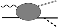
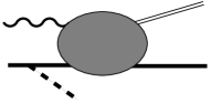
(b)

Figure 8: (a) The mechanism for hard exclusive photo– or electroproduction of a system $a$ (vector meson, heavy quarkonium), accompanied by wide–angle pion production, $\gamma+N\;\rightarrow\;a+\pi+N^{\prime}\;(\mbox{or}\;\Delta)$. The blob denotes the amplitude for the subprocess $\gamma+\pi\rightarrow a+\pi$. (b) Competing reaction mechanisms in which the whole nucleon participates in the hard process, and the pion is emitted from the external baryon lines. These contributions can be suppressed if the pion is emitted under sufficiently large transverse momentum.

As we argued already in Section III, the characteristic scale of this form factor, $m_{2g}^{2}$, is comparable to that of the pion electromagnetic form factor, and the analogy with the nucleon Frankfurt:2002ka suggests that it may be as large as $m_{2g}^{2}\approx 1\,{\rm GeV}^{2}$, see Eq.(17) and after. In any event, the characteristic scale of this form factor is much harder than the transverse momenta which could be generated in the pion–baryon cluster system. This is crucial for our discussion, since it guarantees that the reaction mechanism of interest, Fig. 8a, can be separated from the competing mechanism in which the whole nucleon is involved in the hard process, and the extra pion is emitted by the incoming or outgoing nucleon, see Fig. 8b. Keeping $(p-p^{\prime})^{2}$ small, of order $M_{\pi}^{2}$, and choosing $t=(l^{\prime}-q)^{2}$ sufficiently large ($|{\bf l}_{\perp}|\geq 0.3\ldots 0.4\,{\rm GeV}$), one effectively suppresses contributions of the type of Fig. 8b.

We can write the the modulus squared of the amplitude of the process (52) in the form

$$|M_{\gamma+N\rightarrow a+\pi+N^{\prime}}|^{2} = \frac{4\pi}{y}\;w_{N\rightarrow N^{\prime}}\;d_{\pi N}(y,{\bf k}_{\perp})$$ (53)

$$\times |M_{\gamma+\pi\rightarrow a+\pi}|^{2}.$$

Here $w_{N\rightarrow N^{\prime}}$ is an isospin factor; its value is 1 for $p\rightarrow p$ or $n\rightarrow n$, and 2 for $p\rightarrow n$ or $n\rightarrow p$ transitions. Furthermore, $M_{\gamma+\pi\rightarrow a+\pi}$ denotes the invariant amplitude of the subprocess $\gamma+\pi\rightarrow a+\pi$. The function $d_{\pi N}(y,{\bf k}_{\perp})$ is defined as, up to a factor, the modulus squared of the amplitude for the nucleon to emit a pion, including the pion propagator, averaged (summed) over the incoming (outgoing) nucleon helicities:

$$\frac{4\pi}{y}\;d_{\pi N}(y,{\bf k}_{\perp})\;\;\equiv\;\;\frac{1}{2}\sum_{\lambda\lambda^{\prime}}\frac{g_{\pi NN}^{2}\;|\bar{u}^{\prime}i\gamma_{5}\tau^{a}u|^{2}}{(k^{2}-M_{\pi}^{2})^{2}}.$$ (54)

Explicit calculation gives

$$d_{\pi N}(y,{\bf k}_{\perp})\;\;=\;\;g_{\pi NN}^{2}\frac{s}{(s+M_{\pi}^{2})^{2}},$$ (55)

where $s\equiv(y^{2}M_{N}^{2}+{\bf k}_{\perp}^{2})/\bar{y}=-k^{2}$ is the spacelike pion virtuality. This function can be interpreted as the transverse momentum–dependent distribution of pions in the nucleon. Formally, the integral of Eq.(55) over all ${\bf k}_{\perp}$, multiplied by 3 to account for the isospin degeneracy, gives the total distribution of pions in the nucleon, $H_{\pi}(y,-{\bf\Delta}_{\perp}^{2}=0)$, cf. Eq.(68) for ${\bf\Delta}_{\perp}=0$. Again, it is physically more sensible to consider the distribution of pions (55) in coordinate space. We define the Fourier transform of Eq.(55) as

$$\tilde{d}_{\pi N}(y,{\bf a}_{\perp}) \equiv \int\frac{d^{2}k_{\perp}}{(2\pi)^{2}}\;e^{i({\bf k}_{\perp}{\bf a}_{\perp})}\;d_{\pi N}(y,{\bf k}_{\perp}),$$ (56)

where ${\bf a}_{\perp}$ is a transverse coordinate variable conjugate to ${\bf k}_{\perp}$. At large $|{\bf a}_{\perp}|$ it behaves as

$$\tilde{d}_{\pi N}(y,{\bf a}_{\perp}) \sim \frac{g_{\pi NN}^{2}\,M_{\pi}^{2}}{16\sqrt{2\pi^{3}}}\;\bar{y}\;\sqrt{\frac{|{\bf a}_{\perp}|}{\tilde{\kappa}_{N}}}\;e^{\displaystyle-\tilde{\kappa}_{N}|{\bf a}_{\perp}|},$$ (57)

where

$$\tilde{\kappa}_{N}\;\;\equiv\;\;\sqrt{y^{2}M_{N}^{2}+\bar{y}M_{\pi}^{2}}.$$ (58)

For $y\sim M_{\pi}/M_{N}$ the width of this distribution in transverse space is of the order $1/M_{\pi}$, i.e., much larger than the size of typical configurations in the nucleon, $1/M_{N}$. In this region the exponential dependence could in principle be observed experimentally in the Fourier transform of the cross section of the reaction (52) with respect to ${\bf k_{\perp}}=-{\bf p^{\prime}}_{\perp}$, i.e., the transverse momentum of the outgoing nucleon. Due to the broad distribution of the cross section in $t$ it should be easy to make a cut on $-t_{\rm min}$ which would allow to measure $d_{\pi N}(y,{\bf k_{\perp}})$ in a sufficiently wide range of ${\bf p^{\prime}}_{\perp}$ such that one could reconstruct $\tilde{d}_{\pi N}(y,{\bf a}_{\perp})$. Alternatively, one could model $\tilde{d}_{\pi N}(y,{\bf a}_{\perp})$ in the whole range of $|{\bf a}_{\perp}|$, calculate the Fourier transform, and check how small ${\bf p}^{\prime}_{\perp}$ needs to be in order for the region of $|{\bf a}_{\perp}|$ which we consider as safe to give the dominant contribution. We assume here that for $|{\bf k}_{\perp}|\ll|{\bf k}_{\perp}^{\prime}|$ the dependence of the amplitude of the subprocess $\gamma+\pi\rightarrow a+\pi$ on the transverse momentum of the “initial” pion, ${\bf k}_{\perp}$, can be neglected.

At sufficiently small Bjorken $x$ the hard subprocess $\gamma+\pi\rightarrow a+\pi$ is dominated by the gluon distribution in the pion. Measuring the cross section of the process $\gamma+N\rightarrow a+\pi+N^{\prime}$, and isolating the contribution from pion exchange as described above, one could thus measure the gluon distribution in the pion, including its $t$–dependence (two–gluon form factor). The complete discussion of the cross section of this process, appropriate kinematical cuts, etc. is beyond the scope of the present investigation and will given elsewhere. Here we note only that at sufficiently small $x$ a simple expression can be written for the ratio of the squared amplitudes of the process (52) and the corresponding production process without pion emission:

$$\frac{|M_{\gamma+N\rightarrow a+\pi+N^{\prime}}|^{2}}{|M_{\gamma+N\rightarrow a+N}|^{2}} = \frac{4\pi}{y}\;w_{N\rightarrow N^{\prime}}\;d_{\pi N}(y,{\bf k}_{\perp})$$ (59)

$$\times \left[\frac{\displaystyle(x/y)\;g_{\pi}(x/y,Q^{2})}{\displaystyle xg(x,Q^{2})}\right]^{2}$$

$$\times \left[\frac{\displaystyle\Gamma_{\pi}(t)}{\displaystyle\Gamma(t)}\right]^{2}.$$

Here $Q^{2}$ denotes the scale appropriate for the hard process, see Refs.Frankfurt:1997fj ; Frankfurt:1995jw for a discussion, and $\Gamma_{\pi}(t)$ and $\Gamma(t)$ are the two–gluon form factors of the pion and nucleon, respectively (in both processes $t$ denotes the invariant momentum transfer between the incoming photon and the outgoing vector meson/photon, see Fig. 8a). Since the distribution of pions is not too small for small $y$, and the gluon density in the pion strongly increases with decreasing $x/y$, we expect the cross section for the process (52) to be non-negligible for $y\sim 0.05\ldots 0.1$. In addition, if indeed the two gluon form factor of the pion decreased slowly with $t$ as in Eq. (17), the production rate would decrease with $|{\bf k}^{\prime}_{\perp}|$ only as $\propto 1/|{\bf k^{\prime}_{\perp}}|^{2}$. One may thus expect noticeable rates for pions produced with transverse momenta $|{\bf k}^{\prime}_{\perp}|\geq 2\,{\rm GeV}$, which is within the acceptance of the current HERA detectors.

VII Conclusions and outlook

In this paper we have studied the role of the pion cloud of the nucleon for the gluon density at large transverse distances. We have identified a specific contribution to the gluon density of transverse size $1/M_{\pi}$, due to soft–pion exchange, which becomes “visible” for $x\ll M_{\pi}/M_{N}$. This results in a finite increase of the average transverse size of the nucleon as $x$ drops significantly below $M_{\pi}/M_{N}$, in agreement with the observed change of the $t$–dependence of the $J/\psi$ photoproduction cross section with incident energy. While this phenomenon has been described previously at the qualitative level, the present investigation shows that with the phenomenological parameters for soft–pion exchange one indeed obtains a consistent quantitative picture.

Let us summarize again in which range of $x$ the soft–pion exchange contribution to the gluon density is meaningful. We have seen that this mechanism sets in for $x<M_{\pi}/M_{N}\sim 10^{-1}$, when the relativistic kinematics allows the pions to propagate distances of order $1/M_{\pi}$ in the transverse plane. It grows to its full strength for $x\lesssim 10^{-2}$, when the momentum fraction of the gluons relative to the pions becomes small ($\sim 10^{-1}$). In principle this contribution to the gluon density survives down to considerably smaller values of $x$. However, for such values of $x$ other effects such as multi-step Gribov diffusion become dominant.

The gluon density at large transverse distances is an important element of the structure of the nucleon which can be calculated theoretically in a model–independent fashion. It can be probed in exclusive processes such as $J/\psi$ photoproduction, or hard electroproduction of real photons or vector mesons at small $x$, by isolating contributions from large impact parameters through measurement of the $t$–dependence. The QCD factorization theorem guarantees that this feature of the nucleon is process–independent as long as the conditions for factorization are met. A particularly promising way of accessing the glue at large transverse distances appears to be hard exclusive production off the nucleon with associated “pion knockout”, which should be possible to observe at HERA.

Our results for the asymptotic behavior of the gluon density at large transverse distances provide model–independent constraints for parametrizations or dynamical models of the impact parameter dependence of the nucleon’s gluon density. Such parametrizations are needed to describe e.g. diffractive Higgs production in proton–proton collisions at LHC energies FELIX .

The techniques developed in the present paper can readily be extended to quark distributions, including polarized distributions. The large–$b$ limit of these distributions is in principle also due to soft–pion exchange, and can be described in a model–independent way. However, the minimum number of exchanged pions in the $t$–channel depends on the $G$–parity of the operator measuring the parton distribution, and the relevance of the asymptotic region for eventual observable physical phenomena needs to be studied case–by–case. The impact parameter representation of parton distributions is also useful in connection with specific dynamical models of the nucleon, as it leads to new insights into the dynamical origin of these quantities. For example, with regard to the flavor asymmetry in the nucleon’s sea quark distributions, $\bar{u}(x)-\bar{d}(x)$ and $\Delta\bar{u}(x)-\Delta\bar{d}(x)$, it may help to resolve the long-standing issue to which extent these asymmetries are due to the pion cloud of the nucleon, or to Pauli blocking by the valence quarks Fries:2002um .

In the present investigation we have limited ourselves to the generalized parton distributions at zero longitudinal momentum transfer (zero “skewedness”), which is sufficient for studying the impact parameter dependence of the usual parton densities in the nucleon. The inclusion of skewedness effects is an important problem which we leave for future treatment. In particular, this would allow to include into the considerations a much wider range of experiments, such as deeply–virtual Compton scattering or meson production (pseudoscalar and vector) in the valence region. First steps have been taken to extend the impact parameter representation to generalized parton distributions at non-zero skewedness Diehl:2002he ; however, one is still lacking a simple interpretation as is available in the diagonal case.

We are grateful to H. Weigert for inspiration and help during the initial stages of this work, and to M. Burkardt, L. L. Frankfurt, A. Freund, N. Kivel, G. A. Miller, M. V. Polyakov, A. V. Radyushkin, A. Schäfer, W. Söldner, and M. Stratmann for interesting discussions. We thank the Institute for Nuclear Theory at the University of Washington for its hospitality during the time in which this work was completed. M. S. is an Alexander–von–Humboldt Fellow. C. W. is a Heisenberg Fellow (Deutsche Forschungsgemeinschaft). This work has been supported by D.O.E.

Appendix A Distribution of pions in the nucleon at large impact parameters

A.1 Evaluation of the pion exchange graphs

In this appendix we outline the derivation of the asymptotic behavior of the “parton distribution” of pions in the nucleon at large impact parameters. We first consider the distributions obtained with $N$ intermediate states only; the $\Delta$ contributions will be included subsequently.

In the limit of large transverse distances it is justified to treat the nucleon and the pion as pointlike elementary particles. We assume a pion–nucleon coupling of pseudoscalar form

$$L_{\pi NN}\;\;=\;\;g_{\pi NN}\bar{N}i\gamma_{5}\tau^{a}\pi^{a}N,$$ (60)

where $\tau^{a}$ are the isospin Pauli matrices. The result for the large–$b$ behavior is in fact independent of the type of coupling; i.e. it is the same for all couplings which are equivalent in the soft–pion limit.

We first evaluate the $t$–dependent distributions of pions in the nucleon, as defined by Eq.(21). The nucleon matrix element of the pion light–ray operator is computed using standard Feynman rules,

$$\langle N(P+\Delta/2)|\;\pi^{a}(-\lambda n/2)\pi^{a}(\lambda n/2)\;|N(P-\Delta/2)\rangle$$ (61)

$$= 3ig_{\pi NN}^{2}\;\int\frac{d^{4}k}{(2\pi)^{4}}\;\left[e^{-i\lambda(kn)}+e^{i\lambda(kn)}\right]$$

$$\times \frac{1}{\left[(k+\Delta/2)^{2}-M_{\pi}^{2}+i0\right]\left[(k-\Delta/2)^{2}-M_{\pi}^{2}+i0\right]}$$

$$\times \frac{\bar{u}^{\prime}\;i\gamma_{5}\;(\hat{P}-\hat{k}+M_{N})\;i\gamma_{5}\;u}{\left[(P-k)^{2}-M_{N}^{2}+i0\right]}.$$

The factor 3 arises from the summation over the pion isospin projection. In order to read off the expressions for the distribution functions we have to convert the Dirac structures in the numerator to the form of the L.H.S. of Eq.(21). The $\gamma_{5}$ matrices can be eliminated using the anticommutation relations. The integral over the $\hat{k}$ term can be projected on the structures $\hat{P},\hat{\Delta}$ and $\hat{n}$ by appropriate projections of the four–vector $k$. Finally, we use the identities $\bar{u}^{\prime}\hat{P}u=M_{N}\bar{u}^{\prime}u$ and $\bar{u}^{\prime}\hat{\Delta}u=0$, as well as

$$\frac{P_{\nu}}{M_{N}}\bar{u}^{\prime}u\;\;=\;\;\bar{u}^{\prime}\gamma_{\nu}u-\frac{1}{2M_{N}}\bar{u}^{\prime}\sigma_{\mu\nu}\Delta^{\mu}u,$$ (62)

which follow from the Dirac equation for the external nucleon spinors. The net result is that we can replace in Eq.(61)

$$\bar{u}^{\prime}\;i\gamma_{5}\;(\hat{P}-\hat{k}+M_{N})\;i\gamma_{5}\;u$$ (63)

$$\rightarrow \frac{1}{(Pn)}\left[-(kP)\;+\;(P^{2}-M_{N}^{2})\frac{(kn)}{(Pn)}\right]\bar{u}^{\prime}\hat{n}u$$

$$+ \frac{M_{N}(kn)}{2(Pn)^{2}}\bar{u}^{\prime}\sigma_{\mu\nu}\Delta^{\mu}n^{\nu}u.$$

To get the distribution of pions as a function of the momentum fraction $y$ we still have to compute the Fourier transform of Eq.(61) with respect to the longitudinal distance variable $\lambda$, see Eq.(21). The integral of the combined exponential factors results in delta functions,

$$\int_{-\infty}^{\infty}\frac{d\lambda}{2\pi}\;e^{i\lambda y(Pn)}\;e^{\mp i\lambda(kn)}\;\;=\;\;\delta\!\left[y(Pn)\mp(kn)\right].$$ (64)

Combining everything, we see that the distribution of pions resulting from $N$ intermediate states is given in covariant form by

$$H_{\pi N}(y,t) = 6\,ig_{\pi NN}^{2}\;(Pn)y\;\int\frac{d^{4}k}{(2\pi)^{4}}\delta\!\left[y(Pn)-(kn)\right]$$ (65)

$$\times \frac{1}{\left[(k+\Delta/2)^{2}-M_{\pi}^{2}+i0\right]}$$

$$\times \frac{1}{\left[(k-\Delta/2)^{2}-M_{\pi}^{2}+i0\right]}$$

$$\times \frac{1}{\left[(P-k)^{2}-M_{N}^{2}+i0\right]}$$

$$\times \left[-(kP)\;\;-\;\frac{(kn)}{(Pn)}\,\frac{\Delta^{2}}{4}\right]$$

$$- (y\rightarrow-y),$$

where $t=\Delta^{2}$. For the helicity–flip distribution $E_{\pi N}(y,t)$ the expression in brackets in the next–to–last last line should be replaced by $M_{N}^{2}(kn)/(Pn)$. In the following we quote only the results for the distribution $H_{\pi N}$ used in the present investigation; the corresponding expressions for $E_{\pi N}$ can be derived analogously.

To evaluate the momentum integral we choose the frame described in Section II, where $n^{\mu}=(1,0,0,-1)$, $nP=P^{+}$, and ${\bf P}_{\perp}=0$, see Eqs.(9), which implies $P^{-}=P^{2}/P^{+}$. Furthermore, $\Delta^{+}=\Delta^{-}=0$, and thus ${\bf\Delta}_{\perp}^{2}=-t$. Corresponding light-like components are introduced for the loop momentum, $k$. The integral over $k^{+}$ is taken trivially; the delta function restricts $k^{+}$ to $yP^{+}$. The integral over $k^{-}$ is then performed using Cauchy’s theorem. The poles of the three propagators are located at

$$k^{-} = \frac{({\bf k}_{\perp}\pm{\bf\Delta_{\perp}}/2)^{2}+M_{\pi}^{2}-i0}{yP^{+}},$$ (66)

$$k^{-} = \frac{-{\bf k}_{\perp}^{2}-yM_{N}^{2}+\bar{y}{\bf\Delta}_{\perp}^{2}/4+i0}{\bar{y}P^{+}}.$$ (67)

The integral is non-zero only if the poles lie on different sides of the real axis, which implies $y\bar{y}>0$, or $0<y<1$. Closing the contour in the upper half-plane, encircling the pole (67), we obtain for $0<y<1$

$$H_{\pi N}(y,-{\bf\Delta}_{\perp}^{2}) = \frac{3g_{\pi NN}^{2}}{8\pi}\;\frac{y}{\bar{y}}\;\int\frac{d^{2}k_{\perp}}{(2\pi)^{2}}$$ (68)

$$\times \frac{s_{+}+s_{-}-\bar{y}{\bf\Delta}_{\perp}^{2}}{(s_{+}+M_{\pi}^{2})(s_{-}+M_{\pi}^{2})},$$

where

$$s_{\pm} \equiv \frac{1}{\bar{y}}\left[({\bf k}_{\perp}\pm\bar{y}{\bf\Delta}_{\perp}/2)^{2}+y^{2}M_{N}^{2}\right]$$ (69)

$$= -(k\pm\Delta/2)^{2}\hskip 20.00003pt\mbox{at the pole}$$

are the pion virtualities. The minimum value of the pion virtuality in the loop is

$$s_{{\rm min},N}\;\;=\;\;\frac{y^{2}M_{N}^{2}}{\bar{y}}.$$ (70)

For ${\bf\Delta}_{\perp}=0$ our result (68) reduces to the well–known expression for the isoscalar distribution of pions in the meson cloud model, $f_{\pi N}(y)$ of Ref.Koepf:1995yh , up to form factors at the pion–nucleon vertices, which are not needed in our approach, see below. Note that in Ref.Koepf:1995yh the isospin factor $3$ is included in the definition of $g_{\pi NN}$.

In Eq.(68) it is assumed that $0<y<1$; the distribution for $-1<y<0$ follows trivially from $H_{\pi N}(-y,-{\bf\Delta}_{\perp}^{2})=-H_{\pi N}(y,-{\bf\Delta}_{\perp}^{2})$. In the following, for simplicity, we shall always assume that $0<y<1$, and that the distribution at negative $y$ is restored in this way.

The transverse momentum integral in Eq.(68) for the distribution $H_{\pi}(y,-{\bf\Delta}_{\perp}^{2})$ is logarithmically divergent. However, this divergence is irrelevant for the large–$b$ behavior of the corresponding impact parameter–dependent distribution. It could be removed by subtracting the function at $-{\bf\Delta}_{\perp}^{2}=t=0$,

$$H_{\pi N}(y,-{\bf\Delta}_{\perp}^{2})\;\;\rightarrow\;\;H_{\pi N}(y,-{\bf\Delta}_{\perp}^{2})-H_{\pi N}(y,0).$$ (71)

In impact parameter space this would amount to subtracting a delta function at ${\bf b}=0$, which is irrelevant at large $b$. With the saddle point method employed below, we do not need to perform this subtraction explicitly.

For deriving the large–$b$ behavior of the corresponding impact parameter–dependent distributions it is convenient to introduce the integral representation

$$\frac{1}{A}\;\;=\;\;\int_{0}^{\infty}\!d\alpha\;e^{-\alpha A}\hskip 30.00005pt(A>0)$$ (72)

for the ${\bf k}_{\perp}$–dependent denominators in Eq.(68). The integral over ${\bf k}_{\perp}$ then reduces to a Gaussian integral, which can be computed. We obtain

$$H_{\pi N}(y,-{\bf\Delta}_{\perp}^{2})$$ (73)

$$= \frac{3g_{\pi NN}^{2}}{16\pi^{2}}\;y\;\int_{0}^{\infty}\!d\alpha\;\int_{0}^{\infty}\!d\beta\;$$

$$\times \exp\left[-(\alpha+\beta)(s_{{\rm min},N}+M_{\pi}^{2})-\frac{\alpha\beta}{\alpha+\beta}\bar{y}{\bf\Delta}_{\perp}^{2}\right]$$

$$\times \frac{1}{\alpha+\beta}\left[\frac{1}{\alpha+\beta}+s_{{\rm min},N}-\frac{\alpha\beta}{(\alpha+\beta)^{2}}\bar{y}{\bf\Delta}_{\perp}^{2}\right],$$

where $s_{{\rm min},N}$ is defined in Eq.(70). We can now pass to the impact parameter–dependent distribution of pions in the nucleon, cf. Eq.(23). The Fourier transform of Eq.(73) with respect to ${\bf\Delta}_{\perp}$ is again a Gaussian integral. We get

$$f_{\pi N}(y,b)$$ (74)

$$= \frac{3g_{\pi NN}^{2}}{64\pi^{3}}\;\frac{y}{\bar{y}}\;\int_{0}^{\infty}\!d\alpha\;\int_{0}^{\infty}\!d\beta\;$$

$$\times \exp\left[-(\alpha+\beta)(s_{{\rm min},N}+M_{\pi}^{2})-\frac{\alpha+\beta}{\alpha\beta}\;\frac{b^{2}}{4\bar{y}}\right]$$

$$\times \frac{1}{\alpha\beta}\left(s_{{\rm min},N}+\frac{1}{\alpha\beta}\;\frac{b^{2}}{4\bar{y}}\right).$$

In this representation the large–$b$ asymptotics can be studied using the saddle point method. The stationary point of the exponent is at

$$\alpha\;\;=\;\;\beta\;\;=\;\;\frac{b}{2}\left[\bar{y}\,(s_{{\rm min},N}+M_{\pi}^{2})\right]^{-1/2},$$ (75)

and one immediately sees that with exponential accuracy the large–$b$ asymptotics is given by

$$f_{\pi N}(y,b)\;\;\sim\;\;e^{\displaystyle-\kappa_{N}b},$$ (76)

with

$$\kappa_{N} \equiv 2\left(\frac{s_{{\rm min},N}+M_{\pi}^{2}}{\bar{y}}\right)^{1/2}.$$ (77)

One can easily determine the pre-exponential factor by computing the Gaussian integral over deviations from the stationary point; the result is given in Eq.(24). Alternatively, one can express the integral Eq.(74) in terms of modified Bessel functions,

$$f_{\pi N}(y,b) = \frac{3g_{\pi NN}^{2}}{16\pi^{3}}\;\frac{y}{\bar{y}}\left\{s_{{\rm min},N}\;\left[K_{0}(\kappa_{N}b/2)\right]^{2}\right.$$ (78)

$$+ \left.(s_{{\rm min},N}+M_{\pi}^{2})\;\left[K_{1}(\kappa_{N}b/2)\right]^{2}\right\},$$

and recover the asymptotic behavior Eq.(24) by substituting the asymptotic expressions for the Bessel functions at large arguments. In particular, in this way one can get also the subleading corrections to the pre-exponential factor involving higher powers of $1/(\kappa_{N}b)$, which are more difficult to compute using the saddle point method.

A.2 Large–$b$ behavior from $t$–singularities

The large–$b$ behavior of the distribution of pions in the nucleon can also be derived in an alternative way, which directly exhibits the connection of the large–$b$ asymptotics with the singularities of the pion and nucleon propagators in the Feynman integral (65). Performing in Eq.(23) the integral over the angle between the transverse vectors ${\bf\Delta}_{\perp}$ and ${\bf b}$ we obtain (here $\Delta_{\perp}\equiv|{\bf\Delta}_{\perp}|$)

$$f_{\pi N}(y,b)\;\;=\;\;\int_{0}^{\infty}\frac{d\Delta_{\perp}}{2\pi}\;\Delta_{\perp}\;J_{0}(b\Delta_{\perp})\;H_{\pi N}(y,-\Delta_{\perp}^{2}),$$ (79)

where $J_{0}$ denotes the Bessel function. Substituting the latter by its asymptotic form for large arguments, $J_{0}(b\Delta_{\perp})\sim(2\pi b\Delta_{\perp})^{-1/2}\left[e^{i(b\Delta_{\perp}-\pi/4)}+e^{-i(b\Delta_{\perp}-\pi/4)}\right]$, and rotating the integration contour in the complex $\Delta_{\perp}$ plane to run along the positive (negative) imaginary axis in the integral with the first (second) exponential factor, setting $\Delta_{\perp}=\pm i\delta+0$ with $\delta\geq 0$ real, we get

$$f_{\pi N}(y,b) = \frac{1}{\sqrt{2\pi b}}\;\int_{\mbox{\scriptsize threshold}}^{\infty}d\delta\;\sqrt{\delta}\;e^{-b\delta}\;$$ (80)

$$\times \frac{1}{\pi}\,\mbox{Im}\,H_{\pi N}(y,\delta^{2}+i0).$$

The large–$b$ behavior of the impact parameter–dependent distribution is governed by the threshold behavior of the imaginary part of the $t$–dependent distribution of pions, $H_{\pi N}(y,t)$, which appears for some nonzero positive $t$. The imaginary part can directly be computed from the Feynman integral (65) using the Cutkosky rules, replacing the propagators by appropriate delta functions. One finds that the $t$–channel cut starts at $\delta=\kappa_{N}$, and that the leading threshold behavior of the imaginary part for $\delta\rightarrow\kappa_{N}+0$ is

$$\frac{1}{\pi}\,\mbox{Im}\,H_{\pi N}(y,\delta^{2}+i0) = \frac{3g_{\pi NN}^{2}}{16\pi^{2}}\;\frac{y}{\bar{y}}\left(2s_{{\rm min},N}+M_{\pi}^{2}\right)$$ (81)

$$\times \left[\frac{2}{\kappa_{N}^{3}(\delta-\kappa_{N})}\right]^{1/2}.$$

Substituting this in Eq.(80) and computing the integral over $\delta$, one obtains the asymptotic behavior quoted in Eq.(24).

A.3 The $\Delta$ contribution

The calculation of the contribution from $\Delta$ intermediate states proceeds along the same lines as that of the $N$ contribution; we only outline the essential steps. We assume a $\pi N\Delta$ interaction Lagrangian of the form

$$L_{\pi N\Delta} = \frac{ig_{\pi N\Delta}}{\sqrt{2}M_{N}}\left[\bar{p}\;\partial_{\mu}\pi^{-}\;\Delta_{\mu}^{++}+\sqrt{\frac{2}{3}}\;\bar{p}\;\partial^{\mu}\pi^{0}\;\Delta^{+}_{\mu}\right.$$ (82)

$$+ \left.\frac{1}{\sqrt{3}}\;\bar{p}\;\partial^{\mu}\pi^{+}\;\Delta^{0}_{\mu}\;\;+\;\;\mbox{h.c.}\;\;+\ldots\right],$$

where $p$ is the proton field (we skip the terms for the neutron), and $\Delta_{\mu}$ the spin–3/2 Rarita–Schwinger field describing the $\Delta$ resonance [not to be confused with the four–vector of the momentum transfer in the matrix element (61)]. Our definition of the coupling constant $g_{\pi N\Delta}$ corresponds to that of Ref.Adkins:1983ya , and differs from the one used by Koepf et al. Koepf:1995yh , $(g_{\pi N\Delta})_{\mbox{\scriptsize Koepf et al.}}=\sqrt{2}\;(g_{\pi N\Delta})_{\mbox{\scriptsize this work}}$. The relative coefficients of the terms in Eq.(82) are dictated by isospin invariance. One sees that the total distribution of pions in the proton (i.e., the sum of distributions of $\pi^{+},\pi^{-}$ and $\pi^{0}$) resulting from $\Delta$ intermediate states is equal to the $\pi^{-}\Delta^{++}$ contribution multiplied by $(1+2/3+1/3)=2$.

It the calculation of the Feynman graphs for the $\Delta$ contribution, we use the propagator of the spin–3/2 Rarita–Schwinger field in the form ($l$ is the momentum)

$$\frac{\hat{l}+M_{\Delta}}{l^{2}-M_{\Delta}^{2}+i0}\left[-g_{\mu\nu}+\frac{1}{3}\gamma_{\mu}\gamma_{\nu}+\frac{2}{3M_{\Delta}^{2}}l_{\mu}l_{\nu}\right.$$

$$-\left.\frac{1}{3M_{\Delta}}(l_{\mu}\gamma_{\nu}-\gamma_{\mu}l_{\nu})\right].$$ (83)

After projecting on the Dirac structures appearing in the L.H.S. of Eq.(21), in analogy to the $N$ case, we get [cf. Eq.(65)]

$$H_{\pi\Delta}(y,t)$$ (84)

$$= \frac{4\,ig_{\pi N\Delta}^{2}}{3\,M_{N}^{2}\,M_{\Delta}^{2}}\;(Pn)y\;\int\frac{d^{4}k}{(2\pi)^{4}}\delta\!\left[y(Pn)-(kn)\right]$$

$$\times \frac{1}{\left[(k+\Delta/2)^{2}-M_{\pi}^{2}+i0\right]}$$

$$\times \frac{1}{\left[(k-\Delta/2)^{2}-M_{\pi}^{2}+i0\right]}$$

$$\times \frac{1}{\left[(P-k)^{2}-M_{\Delta}^{2}+i0\right]}$$

$$\times \left[(P-k,k)^{2}-(k\Delta)^{2}/4+M_{\Delta}^{2}(-k^{2}+\Delta^{2}/4)\right]$$

$$\times \left[-(kP)-\frac{(kn)}{(Pn)}\,\frac{\Delta^{2}}{4}+M_{N}(M_{N}+M_{\Delta})\right]$$

$$- (y\rightarrow-y).$$

For the helicity–flip distribution $E_{\pi\Delta}(y,t)$ the expression in the bracket in the next–to–last line should be replaced by $\left[M_{N}^{2}(kn)/(Pn)-M_{N}(M_{N}+M_{\Delta})\right]$. Introducing light–like coordinates as above, and taking the integral over $k^{-}$ using Cauchy’s theorem, we finally get, for $0<y<1$ [cf. Eq.(68)]

$$H_{\pi\Delta}(y,-{\bf\Delta}_{\perp}^{2})$$ (85)

$$= \frac{g_{\pi N\Delta}^{2}}{48\pi\,M_{N}^{2}\,M_{\Delta}^{2}}\frac{y}{\bar{y}}\int\frac{d^{2}k_{\perp}}{(2\pi)^{2}}\frac{1}{(s_{+}+M_{\pi}^{2})(s_{-}+M_{\pi}^{2})}$$

$$\times \left[2M_{\Delta}^{2}(s_{+}+s_{-}-{\bf\Delta}_{\perp}^{2})\right.$$

$$\left.+\;(s_{+}-M_{\Delta}^{2}+M_{N}^{2})(s_{-}-M_{\Delta}^{2}+M_{N}^{2})\right]$$

$$\times \left[2(M_{\Delta}+M_{N})^{2}+s_{+}+s_{-}-\bar{y}{\bf\Delta}_{\perp}^{2}\right],$$

where now the pion virtualities are given by

$$s_{\pm}\;\;\equiv\;\;\frac{1}{\bar{y}}({\bf k}_{\perp}\pm\bar{y}{\bf\Delta}_{\perp}/2)^{2}+s_{{\rm min},\Delta},$$ (86)

with

$$s_{{\rm min},\Delta}\;\;\equiv\;\;\frac{1}{\bar{y}}\left[y^{2}M_{N}^{2}+y(M_{\Delta}^{2}-M_{N}^{2})\right].$$ (87)

For zero momentum transfer, ${\bf\Delta}_{\perp}=0$, Eq.(85) reduces to the $\Delta$ contribution to the isoscalar distribution of pions in the meson cloud model quoted in Ref.Koepf:1995yh [cf. the comment on the different conventions for $g_{\pi N\Delta}$ after Eq.(82)], up to form factors at the $\pi N\Delta$ vertices, which are not needed in our approach. Again, we are interested in Eq.(85) only as a means to derive the large–$b$ asymptotics of the corresponding impact parameter–dependent distribution. This is done in complete analogy to the $N$ case, using the integral representation (72) to convert Eq.(85) to a Gaussian integral. For reference, we quote the result for the $b$–dependent distribution, corresponding to Eq.(74):

$$f_{\pi\Delta}(y,b)$$ (88)

$$= \frac{g_{\pi N\Delta}^{2}}{384\pi^{3}M_{N}^{2}M_{\Delta}^{2}}\;\frac{y}{\bar{y}}\;\int_{0}^{\infty}\!d\alpha\;\int_{0}^{\infty}\!d\beta\;$$

$$\times \exp\left[-(\alpha+\beta)(s_{{\rm min},\Delta}+M_{\pi}^{2})-\frac{\alpha+\beta}{\alpha\beta}\;\frac{b^{2}}{4\bar{y}}\right]$$

$$\times \frac{1}{\alpha\beta}\left\{(X+A_{+}^{2})\left[(X+A_{+}^{2})(X+A_{-}^{2})\phantom{\frac{0}{0}}\right.\right.$$

$$+ \left.\left.\frac{(\alpha+\beta)^{2}}{\alpha\beta}\,X\,A_{+}A_{-}\right]+\ldots\right\},$$

where

$$X \equiv \frac{b^{2}}{4\alpha\beta\bar{y}},$$ (89)

$$A_{\pm}^{2} \equiv s_{{\rm min},\Delta}+(M_{\Delta}\pm M_{N})^{2}$$ (90)

$$= \frac{(M_{\Delta}\pm\bar{y}M_{N})^{2}}{\bar{y}}.$$

The ellipsis in Eq.(88) denotes terms which produce only subleading corrections in $1/b$ to the pre-exponential factor in the large–$b$ asymptotics, which we have not written out for brevity. The large–$b$ behavior can again be studied using the saddle point method; the exponential decay constant is given by Eq.(77) with $s_{{\rm min,N}}$ replaced by $s_{{\rm min,\Delta}}$. The result for the leading large–$b$ behavior is quoted in Eq.(40). Note also that the representation (88) can be used for direct numerical evaluation of $f_{\pi\Delta}(y,b)$.

References

- (1) D. Müller, D. Robaschik, B. Geyer, F. M. Dittes and J. Horejsi, Fortsch. Phys. 42, 101 (1994).
- (2) X. D. Ji, Phys. Rev. D 55, 7114 (1997).
- (3) A. V. Radyushkin, Phys. Rev. D 56, 5524 (1997).
- (4) J. C. Collins, L. Frankfurt and M. Strikman, Phys. Rev. D 56, 2982 (1997).
- (5) A. V. Radyushkin, Phys. Rev. D 58, 114008 (1998).
- (6) M. Burkardt, Int. J. Mod. Phys. A 18, 173 (2003).
- (7) P. V. Pobylitsa, Phys. Rev. D 66, 094002 (2002).
- (8) M. Burkardt, Phys. Rev. D 66, 114005 (2002); arXiv:hep-ph/0302144 .
- (9) L. Frankfurt, W. Koepf and M. Strikman, Phys. Rev. D 57, 512 (1998).
- (10) A. D. Martin, M. G. Ryskin and T. Teubner, Phys. Lett. B 454, 339 (1999).
- (11) L. L. Frankfurt, M. F. McDermott and M. Strikman, JHEP 9902, 002 (1999); JHEP 0103, 045 (2001).
- (12) L. Frankfurt and M. Strikman, Phys. Rev. D 66, 031502 (2002).
- (13) V. N. Gribov, arXiv:hep-ph/0006158 .
- (14) D. Diakonov, V. Petrov, P. Pobylitsa, M. Polyakov and C. Weiss, Nucl. Phys. B 480 341 (1996); Phys. Rev. D 56 4069 (1997).
- (15) V. Yu. Petrov, P. V. Pobylitsa, M. V. Polyakov, I. Börnig, K. Goeke and C. Weiss, Phys. Rev. D 57 4325 (1998).
- (16) J. D. Sullivan, Phys. Rev. D 5, 1732 (1972); A. W. Thomas, Phys. Lett. B 126, 97 (1983).
- (17) S. Kumano, Phys. Rept. 303, 183 (1998); G. T. Garvey and J. C. Peng, Prog. Part. Nucl. Phys. 47, 203 (2001).
- (18) W. Koepf, L. L. Frankfurt and M. Strikman, Phys. Rev. D 53, 2586 (1996).
- (19) J. Jalilian-Marian, A. Kovner, L. D. McLerran and H. Weigert, Phys. Rev. D 55, 5414 (1997); Nucl. Phys. B 504, 415 (1997); Phys. Rev. D 59, 014014 (1999); Phys. Rev. D 59, 034007 (1999); J. Jalilian-Marian, A. Kovner and H. Weigert, Phys. Rev. D 59, 014015 (1999).
- (20) I. Balitsky, Nucl. Phys. B 463, 99 (1996); I. I. Balitsky and A. V. Belitsky, Nucl. Phys. B 629, 290 (2002).
- (21) Y. V. Kovchegov, Phys. Rev. D 61, 074018 (2000).
- (22) For an overview, see E. Lippmaa et al. [FELIX Collaboration], CERN Report No. LHCC-97-45 (1997); J. Phys. G 28, R117 (2002).
- (23) J. C. Collins and D. E. Soper, Nucl. Phys. B 194, 445 (1982).
- (24) L. Frankfurt and M. Strikman, Phys. Rev. Lett. 63, 1914 (1989) [Erratum-ibid. 64, 815 (1990)].
- (25) M. V. Polyakov and C. Weiss, Phys. Rev. D 60, 114017 (1999).
- (26) I. Zahed and G. E. Brown, Phys. Rept. 142, 1 (1986).
- (27) G. S. Adkins, C. R. Nappi and E. Witten, Nucl. Phys. B 228, 552 (1983).
- (28) M. Glück, E. Reya and I. Schienbein, Eur. Phys. J. C 10, 313 (1999).
- (29) M. Glück, E. Reya and A. Vogt, Z. Phys. C 67, 433 (1995).
- (30) R. Machleidt, K. Holinde and C. Elster, Phys. Rept. 149, 1 (1987).
- (31) S. Munier, A. M. Stasto and A. H. Mueller, Nucl. Phys. B 603, 427 (2001).
- (32) The Electron Ion Collider, White Paper, BNL Report BNL-68933, February 2002.
- (33) L. Frankfurt, M. V. Polyakov, M. Strikman, D. Zhalov and M. Zhalov, in Proceedings of Exclusive Processes at High Momentum Transfer, Newport News, Virginia, 15–18 May 2002, p. 361, arXiv:hep-ph/0211263 .
- (34) L. Frankfurt, W. Koepf and M. Strikman, Phys. Rev. D 54, 3194 (1996).
- (35) M. Diehl, Eur. Phys. J. C 25, 223 (2002).
- (36) For a recent discussion, see: R. J. Fries, A. Schäfer and C. Weiss, arXiv:hep-ph/0204060 .