Topological Defect Density in One-Dimensional
Friedmann–Robertson–Walker Cosmological Model: Corrections
Inferred from the Multi-Josephson-Junction-Loop Experiment

Abstract

The data on a strongly-nonequilibrium superconducting phase transition in the multi-Josephson-junction loop (MJJL), which represents a close analog of one-dimensional Friedmann–Robertson–Walker cosmological model, are used to refine a concentration of topological defects after the phase transitions of Higgs fields in the early Universe. The thermal correlations between the phases of order parameter revealed in MJJL can reduce considerably the expected number of cosmological defects and, thereby, show a new way to resolve the long-standing problem of their excessive concentration.

I Introduction

An important feature of the phase transitions of Higgs fields expected at the early stages of cosmological evolution is formation of topological defects, whose concentration can be roughly estimated as $n\approx 1/\,{\xi}_{\rm eff}^{\,d}.$ Here, $d=$ 3, 2, and 1 for the monopoles, cosmic strings, and domain walls, respectively; and ${\xi}_{\rm eff}$ is the effective correlation length, which is commonly assumed to be less than the cosmological causality horizon, ${\xi}_{\rm eff}\,\lesssim\,c\,/H_{\rm pt}\,,$ where $c$ is the speed of light, and $H_{\rm pt}$ is Hubble constant at the instant of phase transition. So, the resulting concentration of the defects should be

$$n\,\gtrsim\,\left(H_{\rm pt}/c\right){}^{d}\,,$$ (1)

which exceeds considerably the upper limits following from the observational data (e.g. review Klapdor-Kleingrothaus and Zuber (1997)).

For the sake of definiteness, we shall further consider the simplest type of defects—the domain walls. In such a case, their excessive concentration can result in the $t^{2}$-dependence for the evolution of cosmological scale factor, leaving less time for galaxy formation and changing the rate of nucleosynthesis. In addition, the domain walls can produce unreasonably large distortions in the cosmic microwave background radiation Zel’dovich et al. (1974); Gelmini et al. (1989).

A commonly-used approach to resolve the domain-wall problem is to introduce some mechanism of their annihilation, for example, utilizing the concept of the so-called “biased” (or asymmetric) vacuum Zel’dovich et al. (1974). As a result, under appropriate choice of parameters of the fields involved, the regions of “false” (energetically unfavorable) vacuum will quickly disappear, eliminating the corresponding domain walls. (A detailed discussion of the various regimes of evolution can be found in Ref. Gelmini et al. (1989).)

Unfortunately, the concept of the biased vacuum is not sufficiently supported by realistic models of elementary particles. So, it becomes interesting to seek for solution of the problem by another way, namely, to answer the question if there are some mechanisms reducing the commonly-used lower limit on the topological defect concentration (1). To examine the efficiency of formation of the defects by the strongly-nonequilibrium symmetry-breaking phase transitions, a number of experiments was carried out recently in the condensed-matter systems, such as liquid crystals Chuang et al. (1991); Bowick et al. (1994), superfluid ${}^{4}\text{He}$ Dodd et al. (1998) and ${}^{3}\text{He}$ Bäuerle et al. (1996); Ruutu et al. (1996), and superconductors both in the form of bulk samples Carmi and Polturak (1999) and quasi-one-dimensional structures Carmi et al. (2000). (The comprehensive review was given, for example, by Kibble Kibble (2001).)

As was established in the last-mentioned experiment, utilizing the multi-Josephson-junction loop (MJJL) Carmi et al. (2000), the probability of occurrence of various field configurations during the phase transition can be estimated much better if the energy concentrated in the defects is taken into account. The main aim of the present article is to apply this idea to the consideration of cosmological phase transitions and, thereby, to find the range of parameters at which formation of the domain walls can be substantially suppressed even without any assumption of asymmetry (or bias) of the vacuum states.

II Review of the MJJL Experiment

A general scheme of the MJJL experiment is shown in Fig. 1: a thin loop produced of the high-temperature YBa₂Cu₃O${}_{7\text{-}\delta}$ superconductor and interrupted by 214 Josephson junctions at the grain boundaries is rapidly cooled from the normal to superconducting phase (namely, from ${\sim}100$ K to 77 K) .

Figure 1: Sketch of the MJJL experiment.

At $T_{c}=90$ K, the segments separated by junctions become superconducting; however the junctions are still normal and, therefore, the superconducting segments are effectively separate. So, a random phase of the superconducting order parameter should be established in each of them.

At subsequent cooling down to the temperature $T_{cJ}$ (which is $5{\div}7$ K below $T_{c}$), the Josephson junctions also become superconducting, so that a superconducting current $I$ is formed along the entire loop. As a result, the loop will be penetrated by the magnetic flux $\Phi$, which is just the measurable quantity. (This is quite close to the original idea by Zurek Zurek (1985), who proposed to observe a spontaneous rotation produced by the superfluid phase transition in a thin annular tube.)

Because of the phase jumps between the isolated segments formed at the stage when $T_{cJ}<T<T_{c}$, the final magnetic flux through the loop is nonzero and varies randomly from one heating–cooling cycle to another. Its histogram $N_{\Phi}(\Phi)$ derived from 166 cycles is well described by the normal (Gaussian) law with zero average value and standard deviation $7.4\,{\phi}_{0}$ (where ${\phi}_{0}$ is the magnetic flux quantum) .

In fact, the above-written experimental value is unreasonably large: if the phase jumps between the segments would be absolutely independent of each other, then the expected width of the distribution should be only $3.6\,{\phi}_{0}$. On the other hand, the excessive experimental value was satisfactorily explained by the authors of this experiment under assumption that the phases of superconducting order parameter in the isolated segments are correlated to each other so that probability $P({\delta}_{i})$ of phase jump ${\delta}_{i}$ at the $i$’th junction is given by Gibbs law:

$$P({\delta}_{i})\propto\exp[-{E_{J}}({\delta}_{i})/k_{B}T]\,,$$ (2)

where $E_{J}$ is the energy concentrated in the Josephson junction, $T$ is the temperature, and $k_{B}$ is Boltzmann constant.

So, the main conclusion from the results of the above experiment is that the energy concentrated in the defects should be taken into account in calculating the probability of realization of the corresponding field configurations, even if the defects are located at distances exceeding the effective correlation length of the phase transition. In other words, the correlation length represents a size of the minimal domain in which the field must be uniform, but it cannot be considered as the scale beyond which the field states are absolutely independent of each other. Of course, for the correlations at the larger scales to take place, the corresponding regions should have the possibility to interact with each other in the course of the previous evolution, before the phase transition. (For the sake of brevity, we shall call them to be in a coherent state.) The last-mentioned condition is satisfied automatically in the laboratory systems but requires a special consideration in the cosmological applications (see inequality (10) below).

III Cosmological Implications

First of all, we should emphasize close similarity between the symmetry-breaking phase transitions in the multi-Josephson-junction loop, drawn in Fig. 1, and the simplest one-dimensional (1D) Friedmann–Robertson–Walker (FRW) cosmological model. To make the quantitative estimates, let us consider the space–time metric

$$ds^{2}=\>dt^{2}-\,a^{2}(t)\>dx^{2}\vphantom{X_{X}}$$ (3)

(where $a(t)$ is the scale factor of FRW model) and the real scalar field $\varphi$ (simulating Higgs field) whose Lagrangian

$${\cal L}\,(x,t)\,=\,\frac{1}{2}\,\big{[}{\left({\partial}_{t}\varphi\right)}^{2}\!-\,{\left({\partial}_{x}\varphi\right)}^{2}\big{]}\,-\>\frac{\lambda}{4}\,{\big{[}\,{\varphi}^{2}\!-\left({\mu}^{2}/\lambda\right)\big{]}}^{2}$$ (4)

possesses $\mathbb{Z}_{2}$ symmetry group, to be broken by the phase transition. (The resulting topological defects in such a model will be evidently the pointlike domain walls.)

As is known, the stable low-temperature vacuum states of the field (4) are

$${\varphi}_{0}=\,\pm\,\mu\,/\sqrt{\lambda}\>,$$ (5)

while a domain wall between them is described as $\varphi\,(x)=\,\pm\,{\varphi}_{0}\tanh\!\big{[}({\mu}/{\sqrt{2}}\,)\,(x-x_{0})\big{]}$ and involves the energy

$$E=\,\frac{2\,\sqrt{2}}{3}\,\frac{{\mu}^{3}}{\lambda}\;.$$ (6)

(From here on, it will be assumed that thickness of the wall ${\sim}{1/\mu}$ is small in comparison with a characteristic domain size.)

Next, by introducing the conformal time $\eta=\!\int dt/a(t)\,$, the space–time metric (3) can be reduced to the conformally flat form Misner (1969):

$$ds^{2}=a^{2}(t)\,[\,d{\eta}^{2}\!-dx^{2}\,]\,;$$ (7)

so that the light rays ($ds^{2}\!=0$) will be described by the straight lines inclined at $\pm\pi/4\,$: $x=\pm\eta+{\rm const}$.

The entire structure of the space–time can be conveniently presented by the conformal diagram in Fig. 2. Let $\eta\!=\!0$ and $\eta\!=\!{\eta}_{0}$ be the beginning and end of the phase transition, respectively, and $\eta\!=\!{\eta}_{*}$ be the instant of observation. Then, as follows from a simple geometric consideration, ${\eta}_{0}$ is the maximum correlation length; so that

$$N\,=\,({\eta}_{*}\!-{\eta}_{0})/{\eta}_{0}\,\approx\,{\eta}_{*}/{\eta}_{0}\quad(\text{at large }N)$$ (8)

is the minimum number of spatial subregions causally-disconnected during the phase transition. (Their final vacuum states are arbitrarily marked by the arrows.)

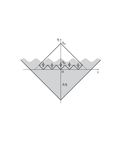
Figure 2: Conformal diagram of the space–time.

A probability of phase transition without formation of the domain walls $P_{N}^{\,0}$ is commonly estimated as ratio of the number of field configurations without domain walls to their total number:

$$P_{N}^{\,0}\,=\,2\,/\,2^{N},$$ (9)

which tends to zero very sharply at large $N$. So, the observable part of the Universe, represented by the large upper triangle in Fig. 2, will inevitably contain a considerable number of the domain walls.

On the other hand, if a sufficiently long interval of the conformal time

$$\Delta\eta\,\geq\,{\eta}_{*}$$ (10)

preceded the phase transition, then a coherent state of the Higgs field (shown by the lower shaded triangle) will be formed by the instant $\eta\!=\!0$ in the entire region observable at $\eta\!=\!{\eta}_{*}$.

The inequality (10) can be satisfied, particularly, in the case of sufficiently long de Sitter stage. Really, if $\,a(t)=\exp(Ht)$, then

$$\eta\,=\,-\,\frac{1}{H}\,e^{-Ht}+{\rm const}\,\to\,-\infty\quad\text{at}\quad t\,\to\,-\infty\,;$$ (11)

so that $\Delta\eta$ can be sufficiently large. From the viewpoint of elementary-particle physics, the de Sitter stage can be easily realized in the overcooled state of Higgs field just before its first-order phase transition. (Let us remind that just this idea was the basis of the first inflationary models; for more details, see review Linde (1984).)

Next, if condition (10) is satisfied, it is reasonable to assume that the coherent state of the field $\varphi$ will exhibit Gibbs-like correlations (similar to the ones occurring in a superconducting Bose condensate of MJJL) between the all $N$ subregions drawn in Fig. 2. In such a case, the probability $P_{N}^{\,0}$ should be calculated taking into account the Gibbs factors for the field configurations involving domain walls:

$$P_{N}^{\,0}\,=\,2\,/\,Z\>,$$ (12)

where

$$Z\,=\>\sum_{i=1}^{N}\;\sum_{s_{i}=\pm 1}\exp\bigg{\{}\!-\frac{E}{T}\,\sum_{j=1}^{N}\,\frac{1}{2}\,(1-\,s_{j}\,s_{j+1})\bigg{\}}.$$ (13)

Here, $s_{j}$ is the spin-like variable describing a sign of the vacuum state in the $j$’th subregion, $E$ is the domain wall energy, given by (6), and $T$ is the characteristic temperature of the phase transition.

From the mathematical point of view, statistical sum (13) is very similar to the one for Ising model, well studied in the condensed-matter physics (e.g. Ref. Isihara (1971)). Using exactly the same methods (attention should be paid to the appropriate choice of zero energy), we get the final result:

$$P_{N}^{\,0}\,=\,\frac{2}{{\left[1+e^{-E/T}\right]}^{N}+{\left[1-e^{-E/T}\right]}^{N}}\;.$$ (14)

(Yet another method of calculating this quantity, based on explicit expressions for the probabilities of field configurations with various numbers of the domain walls, was presented in our article Dumin (2000).)

As is seen in Fig. 3, $P_{N}^{\,0}$ drops very sharply with increasing $N$ at small values of $E/T$ but becomes a gently decreasing function of $N$ when the parameter $E/T$ is sufficiently large. Therefore, just the large energy concentrated in the domain walls turns out to be the factor substantially suppressing the probability of their formation.

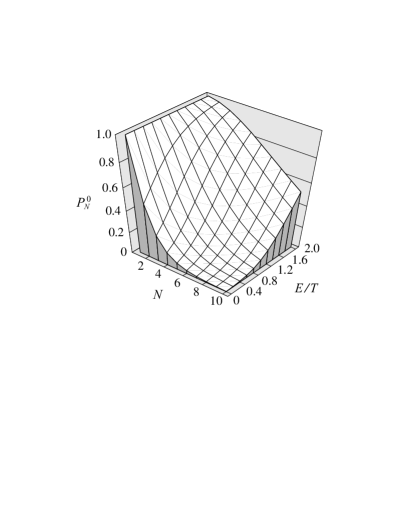
Figure 3: The probability of phase transition without formation of the domain walls $P_{N}^{\,0}$ as function of the number of disconnected subregions $N$ and the ratio of the domain wall energy to the phase transition temperature $E/T$.

As can be easily derived from (14), the probability of absence of the domain walls in the observable region of space–time becomes on the order of unity (for example, $1/2$) if $\,E/T\gtrsim\ln N$ or, by substituting (6) and (8),

$$\frac{{\mu}^{3}}{\lambda\,T}\>\gtrsim\>\ln\frac{{\eta}_{*}}{{\eta}_{0}}\>,$$ (15)

which is just the required inequality, mentioned in Introduction. Because of the very weak logarithmic dependence in the right-hand side of (15), this condition may be quite reasonable for a certain class of field theories.

Moreover, the situation should be even more favorable in the cases of higher spatial dimensions. A well-known property of Ising models in 2 and 3 dimensions is the tendency for aggregation of the domains with the same sign of the order parameter when the temperature drops below some critical value (e.g. Ref. Rumer and Ryvkin (1980)). In the condensed-matter applications, this corresponds to the spontaneous magnetization of a solid body. Regarding the cosmological context, we can expect that probability of formation of the domain walls will be reduced dramatically at the sufficiently large values of $E/T$ . This subject will be discussed in more detail in a separate paper Dumin and Svirskaya (2003).

Although the model under consideration requires a presence of inflationary stage (for the coherent state of Higgs field to be formed ), it is not equivalent to the traditional inflationary models, where decrease in concentration of the previously formed topological defects is a purely geometrical effect, associated with sharp expansion of the space. This raises a problem of new topological defects that can be formed at a subsequent stage of decay of the inflaton field by itself. On the other hand, the inflationary stage in our model results in suppressing formation of the defects (rather than subsequent decrease in their concentration). From this point of view, it represents a self-consistent solution of the problem.