Quark-Antiquark Exchange in $\gamma^{*}\,\gamma^{*}$ Scattering

Abstract:

We calculate the high energy behavior of quark-antiquark exchange in $\gamma^{*}\,\gamma^{*}$ elastic scattering by summing, to all orders, the leading double logarithmic contributions of the QCD ladder diagrams. Motivation comes from the LEP data for $\sigma_{tot}^{\gamma^{*}\,\gamma^{*}}$ which indicate the need for secondary reggeon exchange. We show that, for large photon virtualities, this exchange is calculable in pQCD. This applies, in particular, to parts of the LEP kinematic region.

1 Introduction

The $\gamma^{*}\,\gamma^{*}$ collision at high energies is the unique laboratory for testing asymptotic properties of perturbative QCD. The virtuality of the photons justifies the use of perturbative QCD, and modern electron positron colliders (LEPII, a future linear collider NLC) allow to measure the total cross section of $\gamma^{*}\,\gamma^{*}$ scattering at energies where asymptotic predictions of perturbative QCD can be expected to set in. The dominant contribution to the process is given by the BFKL Pomeron [1] which gives rise to a cross section strongly rising with energy $\sigma_{total}^{\gamma^{*}\,\gamma^{*}}\sim s^{\alpha_{P}(0)}$. Here $\alpha_{P}(0)$ is the Pomeron intercept which, in leading order and for realistic values of the photon virtualities, lies in the region $\alpha_{P}(0)\simeq 0.3\,-\,0.5$.

There is little doubt that the pomeron will dominate at very high energies, and it is expected to be a main contribution at any future linear collider. At present, however, the only source for experimental data on photon photon collisions is LEP [2, 3]. These data are at energies which cannot be considered as asymptotically large, and it has become clear that at LEP energies, the cross section is not yet dominated by the pomeron  [4, 5, 6, 7, 8, 9]. The data rather indicate the necessity to include, in the theoretical description, several corrections. Perturbative corrections are due to the quark box (often referred to as QPM contribution); recently [10] first $O(\alpha_{s})$ corrections to the quark box have been considered. NLO corrections to the BFKL Pomeron are not yet fully available: whereas the NLO corrections to the BFKL kernel have been completed  [11], those of the photon impact factor are not yet finished  [12, 13]. Nonperturbative contributions include the soft Pomeron (in the low-$Q^{2}$ region) and the exchange of secondary reggeons: the exchange of $f_{0}$ (flavor singlet) or $A_{0}$, $A_{2}$ (flavor nonsinglet)  [6, 7, 8]. In this paper we address the latter contributions, the corrections due to secondary reggeons.

In hadron hadron scattering, secondary reggeons denote the exchange of mesons and are of nonperturbative nature. This may change, however, if we replace one of the hadrons (or both) by a virtual photon. We know from the $\gamma^{*}p$ process in deep inelastic electron proton scattering that the rise of the total cross section with energy becomes substantially steeper than in proton proton scattering; this observation has lead to the notion of a ’hard Pomeron’. What makes this hard Pomeron particularly attractive is that its energy dependence becomes calculable in pQCD. In $\gamma^{*}\gamma^{*}$ scattering, the high energy behavior should be described by the BFKL Pomeron, i.e. pQCD provides an absolute prediction for this process. In analogy with this, one might expect that also the secondary exchange may become accessible to a perturbative analysis, if we replace one or both external hadrons by virtual photons. If so, meson exchange will be modelled by the exchange of $q\bar{q}$ ladders [14], and its prediction for the energy dependence may be tested in the corrections to BFKL exchange in $\gamma^{*}\gamma^{*}$ scattering. It is the purpose of this paper (and a forthcoming one) to investigate this possibility more closely. As a start, we present a perturbative QCD calculation of the even-signature flavor nonsinglet contribution to the total $\gamma^{*}\,\gamma^{*}$ cross section. This is done by summing over gluon ladders with two quarks in the $t$-channel. The flavor singlet case appears to be more complicated since it involves the mixing between quark-antiquark and two-gluon states in the t-channel (where the two-gluon state has a helicity content different from the so-called nonsense-helicity configuration in the BFKL Pomeron). The flavor singlet exchange is expected to be somewhat larger than the nonsinglet one [15], and we will come back to it in a forthcoming paper.

One of the striking differences between gluon exchange in the BFKL calculations and quark-antiquark exchange is the appearance of double logarithms [16, 17]. As result of this, the intercept of the $q\bar{q}$-system is of the order $\omega_{0}^{q\bar{q}}\,=\,\sqrt{const\;\alpha_{s}}$ (as opposed to $\omega_{0}^{BFKL}\,=\,const\;\alpha_{s}$ in the single logarithmic high energy behavior of the BFKL Pomeron), and its numerical value can be expected to be large. In fact, for $q\bar{q}$ scattering it is known  [14] that the cross section goes as $\sim s^{\omega_{0}\,-\,1}$ with $\omega_{0}\,=\,\sqrt{2\,\alpha_{s}\,C_{F}/\pi}\simeq 0.5$. It is remarkable that this intercept obtained in pQCD is very close to the nonperturbative one known from phenomenology. For $\gamma^{*}\,\gamma^{*}$ scattering we obtain the same result for the intercept.

Another crucial feature of the double logarithmic calculation is its dependence on the infrared region. In principle, the ladder graphs to be summed are infrared safe. However, quite in analogy with the BFKL approximation, the contribution from small momenta is not believable, and one has to introduce a cutoff scale, $\mu_{0}\leq 1$GeV, which separates the infrared from the large momentum region. Taking the virtualities of the external photons to be sufficiently large and then considering the high energy limit one observes that, for not too large energies, the result is independent of this infrared cutoff: a natural infrared cutoff for the transverse momenta inside the ladder appears, which is of the order $Q^{4}/s$ and decreases with energy. Thus with increasing energy this cutoff eventually reaches the scale $\mu_{0}^{2}$, and the integration starts to penetrate the nonperturbative domain. In this region perturbative QCD cannot be trusted any more. Therefore, for energies $s$ larger than $Q^{4}/\mu_{0}^{2}$ one has to limit the transverse momenta to be larger than $\mu_{0}$, and the perturbative high energy behavior of the $q\bar{q}$ exchange starts to depend upon the cutoff. This dependence turns out to be rather weak: it mainly resides in the pre-exponent and not in the exponent of the energy. In our calculation we will study this dependence in detail: we will compute the sum of double logarithms

$$\sum_{n\geq 1}a_{n}\alpha_{s}^{n-1}\left(\ln^{2}\frac{s}{Q^{2}}\right)^{n}.$$ (1.1)

When $\frac{Q^{4}}{s}$ reaches the cutoff $\mu_{0}^{2}$ another large logarithm appears, $\ln Q^{2}/\mu_{0}^{2}$, which we will include into our analysis:

$$\sum_{n\geq 1}\alpha_{s}^{n-1}\left(a_{n0}\ln^{2n}\frac{s}{Q^{2}}+a_{n1}\ln^{2n-1}\frac{s}{Q^{2}}\ln\frac{Q^{2}}{\mu_{0}^{2}}+...+a_{nn}\ln^{2n}\frac{Q^{2}}{\mu_{0}^{2}}\right).$$ (1.2)

In particular we will study the role of $\mu_{0}^{2}$ in the determination of the pre-exponential behavior of the high energy asymptotics.

The task of the double log resummation in $\gamma^{*}\,\gamma^{*}$ collision can be attacked by several methods. First, we follow the original paper Ref. [16] in which the question of double log resummation $e^{+}e^{-}$ annihilation was addressed first. By direct summation of the ladder graphs this method leads to a Bethe-Salpeter type equation for the amplitude. Compared to the original work of Ref. [16] the case of $\gamma^{*}\,\gamma^{*}$ is slightly more complicated, since the additional scale $Q^{2}$ is involved. This complication results in a more sophisticated structure of the solution. We apply this method to ladder diagrams which are the relevant diagrams for the even-signature exchange. One of our main results is the discovery of the ’hard region’ $\mu_{0}^{2}<Q^{4}/s$ in which pQCD is reliable.

The second method uses the infrared evolution equation (IREE) for the amplitude in the Mellin space. IREE was first derived in Ref. [17] in application to quark-quark scattering, and, more recently, has been applied to the calculation of the small-x behavior of flavor nonsinglet structure functions in Ref. [18] and to polarized structure functions in Refs.  [15, 19]. Within the double log accuracy IREE traces the dependence of the amplitude on the infrared cutoff $\mu$ of the quark transverse momentum in the ladder. The scale $\mu$ is auxiliary in this method. We will see, however, that when identified with the real scale of nonperturbative physics, $\mu_{0}^{2}$, it leads to the same answer as the linear equation of the first approach. Use of IREE allows to discuss not only the even signature case (with ladder diagrams), but also the odd signature case (with non-ladder diagrams).

A third way of handling the quark-antiquark exchange has been described in  [20, 21]: using the partial wave formalism and the notion of the reggeon Green’s function, a linear equation á la BFKL has been found for the fermion-antifermion scattering amplitude. In [21] the kernel has been shown to have the same conformal properties as the BFKL kernel. However, the application of this formulation to our problem is not completely straightforward: the coupling of the quark-antiquark ladder to the external photons involves a careful handling of the double logarithmic integrations. We will show how our result for the hard region can be obtained from the reggeon Greens’s function.

The structure of the paper is following. In the next Section (2) notations are introduced, and the quark box diagram is discussed. In Section 3 we sum the gluon ladder and derive a Bethe-Salpeter type equation for the amplitude. This equation is solved in Section 4. We also discuss the solution and present the high energy asymptotics. In Section 5 we rederive the same result using the method of the infrared evolution equation (IREE). The approach based on the reggeon Green function is discussed in Section 6. Some numerical estimates are given in Section 7. Section 8 contains our conclusions. Two appendixes contain some details of our calculations, supplementing sections 4 and 5.

2 The quark box

We begin with the lowest order diagrams for the scattering amplitude $T^{\gamma^{*}\gamma^{*}}$ of the elastic $\gamma^{*}\gamma^{*}$ scattering process. We restrict ourselves to the forward direction $t=0$, and for simplicity we first take the virtualities of all external photons to be equal.

The exact computation can be found in Ref.[22]; we restrict ourselves to the high energy behavior. The lowest order consists of the three fermion-loop diagrams (Fig. 1, a - c); at high energies only the planar box (a) and its $s\leftrightarrow u$ cross partner (b) contribute to the leading double-logarithmic behavior.

Figure 1: The Born level diagrams.

The calculations below are done using the Feynman gauge. Our method of extracting the double-logs will be close to the original paper  [16]. We introduce the notation (Fig. 1)

$$p_{A}^{2}\,=\,-\,Q^{2}\,;\,\,\,\,\,\,\,\,p_{B}^{2}\,=\,-\,Q^{2}\,;\,\,\,\,\,\,\,\,\,\,(p_{A}\,+\,p_{B})^{2}\,=\,s\,;\,\,\,\,\,\,\,\,\,\,x\,=\,Q^{2}/s\,.\,\,\,\,\,\,\,\,\,.$$ (2.3)

In our Sudakov decomposition $k=\beta q-\alpha p+k_{\perp}$ (with $k_{\perp}^{2}=-\vec{k}^{2}$) the light cone vectors $p$, $q$ are defined through

$$p_{A}\,=\,p\,-\,x\,q\,;\,\,\,\,\,\,\,\,\,\,\,\,\,\,p_{B}\,=\,q\,-\,x\,p\,;\,\,\,\,\,\,\,\,\,\,\,\,\,p^{2}\,=\,q^{2}\,=\,0\,;\,\,\,\,\,\,\,\,\,\,\,\,\,2\,(p\,q)\,=\,s\,.$$ (2.4)

Transverse polarization vectors are defined by $\epsilon_{\pm}^{\mu}\,=\,\frac{1}{\sqrt{2}}\,\left(0,1,\pm i,0\right)$, the longitudinal ones by $\epsilon_{L}(p_{A})\,=\,\frac{1}{\sqrt{Q^{2}}}\,\left(p\,+\,x\,q\right)\,=\,\frac{1}{\sqrt{Q^{2}}}\,\left(p_{A}\,+\,2\,x\,q\right)$,   $\epsilon_{L}(p_{B})\,=\,\frac{1}{\sqrt{Q^{2}}}\,\left(p\,+\,x\,q\right)\,=\,\frac{1}{\sqrt{Q^{2}}}\,\left(p_{B}\,+\,2\,x\,q\right)$.

We first analyze the quantum number structure of the t-channel. We Fierz-transform the upper part of the trace expression:

$$\gamma^{\nu}(k+p_{A})\gamma^{\mu}\,=\,\left((k+p_{A})^{\nu}g^{\mu\rho}\,+\,(k+p_{A})^{\mu}g^{\nu\rho}\,-\,(k+p_{A})^{\rho}g^{\mu\nu}\right)\gamma_{\rho}\,+\,i\epsilon^{\nu\sigma\mu\rho}(k+p_{A})_{\sigma}\gamma_{5}\gamma_{\rho}.$$ (2.5)

As discussed in  [14], the vector current generates the even signature $A_{2}$ exchange, the pseudovector current the $A_{1}$ exchange. The absence of the scalar, pseudoscalar, and tensor currents seems to indicate that, in $\gamma^{*}\gamma^{*}$ scattering, there is no scalar or pseudoscalar ($\pi$-like) exchange; note, however, that the first gluon rung inside the quark loop might contain the axial anomaly, i.e. the coupling of the t-channel pion-like state to two gammas is nonzero. In our subsequent analysis we will restrict ourselves to the vector contribution. The pseudovector exchange as well as the pseudoscalar exchange decouple from the helicity conserving scattering, i.e. is of no interest for the total cross section.

Let us now turn to the quark loop. In order to find a double-logarithmic contribution we need to find, in the trace expression in the numerator, terms proportional the leading power of $s$ and to $k_{\perp}^{2}$. For the numerator of the planar box diagram with transverse polarization we obtain:

$$tr\,\left(\epsilon(A)\,k\,\epsilon(B)\,(k-p_{B})\,\epsilon(B^{\prime})\,k\,\epsilon(A^{\prime})\,(p_{A}+k)\right)\,\approx\,p_{A}\,\cdot\,p_{B}\,\,tr\,\left(\epsilon(A)\,k\,\epsilon(B)\,\epsilon(B^{\prime})\,k\,\epsilon(A^{\prime})\,\right),$$ (2.6)

where, on the rhs, we have made use of the fact that, in the high energy limit, the leading power of $s$ is due to the product $p_{A}\cdot p_{B}$. For the helicity conserving scattering we obtain:

$$tr\,\left(\epsilon(A)\,k\,\epsilon(B)\,(k-p_{B})\,\epsilon(B^{\prime})\,k\,\epsilon(A^{\prime})(p_{A}+k)\right)\,\approx\,2\;s\;k_{\perp}^{2}\,\times$$

(2.7)

$$\left[\epsilon(A)\cdot\epsilon(A^{\prime})\;\;\epsilon(B)\cdot\epsilon(B^{\prime})\;\;+\;\;\epsilon(A)\cdot\epsilon(B^{\prime})\;\;\epsilon(B)\cdot\epsilon(A^{\prime})\;\;-\;\;\epsilon(A)\cdot\epsilon(B)\;\;\epsilon(A^{\prime})\cdot\epsilon(B^{\prime})\right].$$

For the helicity conserving case (which we will need for the total cross section) the last two terms cancel. In the following, therefore, we shall restrict ourselves to the first term of the rhs of (2). For later convenience we define the trace factor:

$$\tau_{TT}\,=\,4\,\,N_{c}\,\,\alpha_{em}^{2}\,\,F_{ns}\;\;\epsilon(A)\,\cdot\,\epsilon(A^{\prime})\;\;\epsilon(B)\,\cdot\,\epsilon(B^{\prime}),$$ (2.8)

where

$$F_{ns}\,\,=\,\,\sum_{quarks}e_{q}^{4}\,\,-\,\,\frac{1}{N_{f}}\,(\sum_{quarks}e_{q}^{2})^{2}$$ (2.9)

denotes the projection on the flavor nonsinglet t-channel (for the flavor group $SU(N_{f})$), and $e_{q}$ stands for the electric charge of the quark, measured in units of $e$.

Diagram Fig. 1b will be obtained by simply substituting, at the end of our calculation, $s\to u$. The nonplanar diagram Fig. 1c has no contribution proportional to $sk_{\perp}^{2}$ and will be neglected.

As to the integration over the momentum $k$, it will be instructive to first follow [16]: taking into account the $k_{\perp}^{2}$ factor from the numerator, we first do the transverse integration (formally by replacing one of the exchange propagators by a $\delta$ function), and are then left with the $\alpha$ and $\beta$-integrals of the type

$$\int\frac{d\alpha}{\alpha}\int\frac{d\beta}{\beta}$$ (2.10)

which are restricted to lie in the region:

$$x\,<\,\alpha\,<\,1,\;\;\,\,\,\,\,\,\,\,\,\,\,\,\,\,x\,<\,\beta\,<\,1,\;\;\,\,\,\,\,\,\,\,\,\,\,\,\,\mu_{0}^{2}\,<\,s\,\alpha\,\beta\,=\,\vec{k}^{2}\,<\,s$$ (2.11)

where $\mu_{0}$ denotes the momentum scale which separates the infrared (nonperturbative) region from the hard region. In the following, however, we will use, as integration variables, $\beta$ and $\vec{k}^{2}$, and the limits have to be derived from (2.11). We have to distinguish between the two kinematic regions which we denote by ‘$+$’ and ‘$-$’:

$$I^{+}:\;\;\mu_{0}^{2}\,<\,\frac{Q^{4}}{s}\\$$ (2.12)

$$I^{-}:\;\;\frac{Q^{4}}{s}\,<\,\mu_{0}^{2}.$$ (2.13)

In the first region, $I^{+}$, we have the following limits of integration

$$\int_{Q^{2}/s}^{1}\frac{d\beta}{\beta}\int_{\beta Q^{2}}^{\beta s}\frac{dk^{2}}{k^{2}}\,\,=\,\,\ln^{2}\frac{s}{Q^{2}}.$$ (2.14)

In the second region, $I^{-}$, we have two separate contributions:

$$\int_{Q^{2}/s}^{\mu_{0}^{2}/Q^{2}}\frac{d\beta}{\beta}\int_{\mu_{0}^{2}}^{\beta s}\frac{dk^{2}}{k^{2}}\,+\,\int_{\mu_{0}^{2}/Q^{2}}^{1}\frac{d\beta}{\beta}\int_{\beta\,Q^{2}}^{\beta s}\frac{dk^{2}}{k^{2}}\,=\,\frac{1}{2}\left(\ln^{2}\frac{s}{Q^{2}}\,-\,\ln^{2}\frac{Q^{2}}{\mu_{0}^{2}}\right)\,+\,\ln\frac{s}{Q^{2}}\ln\frac{Q^{2}}{\mu_{0}^{2}}.$$ (2.15)

One easily verifies that at $\mu_{0}^{2}\,=\,\frac{Q^{4}}{s}$ the two results coincide. All other photon polarizations, at high energies, are suppressed compared to the helicity conserving case of transverse polarization. For example, the case $TL\to TL$ goes as $const$, the case $LL\to LL$ as $1/s$. In the following we will restrict ourselves to the leading polarization, to $TT\to TT$. Combining (2.8) and (2.14), (2.15) we write our result for the planar box diagram in the form

$$T_{box}^{\pm}\,=\,\,\tau_{TT}\,\left\{\begin{array}[]{ll}\ln^{2}\frac{s}{Q^{2}}&\;\;\;\,\,if\;\;\;\,\,\mu_{0}^{2}\,\,<\,\,\frac{Q^{4}}{s}\\ \ln^{2}\frac{s}{Q^{2}}-\frac{1}{2}\left(\ln\frac{s}{Q^{2}}-\ln\frac{Q^{2}}{\mu_{0}^{2}}\right)^{2}&\,\,\;\;\;if\,\,\;\;\;\frac{Q^{4}}{s}\,\,<\,\,\mu_{0}^{2}\end{array}\right\}\,.$$ (2.16)

The nonplanar box in Fig. 1b is obtained by substituting $s\to u$, and in the sum of the two diagrams the obtained results stand for the even signature $A_{2}$ exchange. The total cross section for $\gamma^{*}\,\gamma^{*}$ (averaged over the incoming transverse helicities) follows from

$$\sigma^{\gamma^{*}\,\gamma^{*}}\,=\,\frac{1}{s}\,Im\,T\,\simeq\,\frac{1}{s}\,\frac{\pi\,\partial T}{\partial\ln s}$$ (2.17)

(with the last approximate equality being valid in the high energy approximation only) and has the form

$$\sigma^{\gamma^{*}\,\gamma^{*}}_{Born}\,=\,\tau_{TT}\,\pi\,\left\{\begin{array}[]{ll}2\;\ln\frac{s}{Q^{2}}&\,\,\,\,\,if\;\;\;\,\,\,\,\,\,\,\,\,\,\mu_{0}^{2}\,\,<\,\,\frac{Q^{4}}{s}\\ \ln\frac{s}{\mu_{0}^{2}}&\,\,\,\,\,if\,\,\,\,\,\;\;\;\,\,\,\,\,\frac{Q^{4}}{s}\,\,<\,\,\mu_{0}^{2}\end{array}\right\}\,.$$ (2.18)

It is not difficult to generalize our analysis to the case of unequal photon masses, $Q_{1}^{2}$ and $Q_{2}^{2}$. Instead of the scaling variable $x=Q^{2}/s$ we now have the two variables $x_{i}=Q_{i}^{2}/s$ ($i=1,2$). The integration region (2.11) is replace by

$$x_{2}<\,\alpha\,<\,1,\;\;\,\,\,\,\,\,\,\,\,\,\,\,\,\,x_{1}\,<\,\beta\,<1,\;\;\,\,\,\,\,\,\,\,\,\,\,\,\,\,\,\,\mu_{0}^{2}\,<\,s\,\alpha\,\beta\,=\,\vec{k}^{2}\,<\,s\,.$$ (2.19)

The two kinematic regions (2.12), (2.13) become

$$I^{+}:\;\;\mu_{0}^{2}\,<\,\frac{Q_{1}^{2}\,Q_{2}^{2}}{s}\\$$ (2.20)

$$I^{-}:\;\;\frac{Q_{1}^{2}\,Q_{2}^{2}}{s}\,<\,\mu_{0}^{2},$$ (2.21)

and the result (2.16) for the planar box diagram takes the form:

$$T_{box}^{\pm}\,=\,\,\tau_{TT}\,\left\{\begin{array}[]{ll}\ln\frac{s}{Q_{1}^{2}}\,\ln\frac{s}{Q_{2}^{2}}&\,\,\,\,\,if\;\;\;\,\,\,\,\,\mu_{0}^{2}\,<\,\frac{Q_{1}^{2}\,Q_{2}^{2}}{s}\\ \ln\frac{s}{Q_{1}^{2}}\,\ln\frac{s}{Q_{2}^{2}}\,-\,\frac{1}{2}\,\ln^{2}\frac{s\mu_{0}^{2}}{Q_{1}^{2}\,Q_{2}^{2}}\par&\,\,\,\,\,if\,\,\,\,\,\;\;\;\frac{Q_{1}^{2}Q_{2}^{2}}{s}\,<\,\mu_{0}^{2}\end{array}\right\}\,.$$ (2.22)

3 Linear equations for the ladder

We now turn to higher order corrections to the quark loop diagrams.

For the gluons we will use Feynman gauge, and we make use of the discussion given in  [15, 16, 17, 18, 19, 23]. When selecting those Feynman diagrams which in the high energy limit contribute to the double logarithmic behavior, one has to distinguish between even and odd signature. For the case of quark-quark scattering it has been shown [17] that the even signature amplitude is described by ladder diagrams, whereas the odd signature amplitude has also non-ladder graphs. In this and in the following section we derive and discuss a linear integral equation for the even signature amplitude; so we can restrict ourselves to QCD ladder diagrams. The odd signature case can be derived from the IREE (to be discussed in section 5).

Let us consider the diagram with one gluon rung (Fig. 2a).

(a)	(b)

Figure 2: The first gluon rung (a). The ladder (b).

We begin with the trace and look for terms which result, for each of the two loop momenta $k_{1}$ and $k_{2}$, in a factor $\vec{k}_{i}^{2}$. Writing down the trace we find, for the lower cell, the product $...\gamma_{\mu}\;k_{2}\;\epsilon(B)\;(k\,-\,p_{B})\;\epsilon(B^{\prime})\;k_{2}\;\gamma^{\mu}\;...$ which can be rewritten as $2\,k_{2\;\perp}^{2}\,k_{2}\;\epsilon(B)\;(k\,-\,p_{B})\;\epsilon(B^{\prime})\;k_{2}+...$ where the remainder (indicated by dots), for the helicity conserving case $\epsilon(B)=\epsilon(B^{\prime})$, does not contribute to the double logarithmic approximation. The result for the trace therefore becomes

$$4\,s\,k_{1\;\perp}^{2}\,k_{2\;\perp}^{2}\,\epsilon(A)\,\cdot\,\epsilon(A^{\prime})\;\;\epsilon(B)\,\cdot\,\epsilon(B^{\prime}).$$ (3.23)

The $k^{2}$ factors will cancel against exchange propagators; together with color and $\pi$ factors we obtain the factor

$$\lambda\,\,=\,\,\frac{\alpha_{s}\,C_{F}}{2\,\pi}$$ (3.24)

for the gluon rung.

Turning to the momentum integrations, we, once more, first follow the procedure outlined in  [16] and integrate over the transverse momenta. The remaining $\alpha$ and $\beta$ integrals are of the logarithmic type (2), and the variables are ordered according to $x\,<\,\alpha_{2}\,<\,\alpha_{1}\,<\,1$,   $x\,<\,\beta_{1}\,<\,\beta_{2}\,<\,1$, and their products are restricted by $\mu_{0}^{2}\,<\,s\,\alpha_{i}\,\beta_{i}\,=\,\vec{k}_{i}^{2}\,<\,s$. In what follows, however, we choose the variables $\beta_{i}$, $k_{i}^{2}\,=\,\vec{k}_{i}^{2}$; the integrals to be done are

$$\int\frac{d\beta_{1}}{\beta_{1}}\,\,\int\frac{dk_{1}^{2}}{k_{1}^{2}}\,\,\int\frac{d\beta_{2}}{\beta_{2}}\,\,\int\frac{dk_{2}^{2}}{k_{2}^{2}}$$ (3.25)

with the integration region

$$x\,=\,\frac{Q^{2}}{s}\,<\,\beta_{1}\,<\,\beta_{2}\,<\,1,\;\;\,\,max(\beta_{2}\,Q^{2},\,\mu_{0}^{2})\,<\,k_{2}^{2}\,<\,\beta_{2}\,s,\,\,\;\;max(\frac{k_{2}^{2}\,\beta_{1}}{\beta_{2}},\,\mu_{0}^{2})\,<\,k_{1}^{2}\,<\,\beta_{1}\,s\,.$$ (3.26)

As in the one loop case, we shall see that the two possibilities (2.12) and (2.13) will have to be distinguished. We start with the integration of the upper cell, keeping the variables of the lower cell, $\beta_{2}$, $k_{2}^{2}$, fixed. The restrictions (3.26) imply two distinct regions (Fig. 3):

$$I_{2}^{+}:\;\;\;\mu_{0}^{2}\,\,<\,\,\frac{Q^{2}\,k_{2}^{2}}{s\,\beta_{2}}\\$$ (3.27)

$$I_{2}^{-}:\;\;\;\frac{Q^{2}\,k_{2}^{2}}{s\,\beta_{2}}\,\,<\,\,\mu_{0}^{2}\,.$$ (3.28)

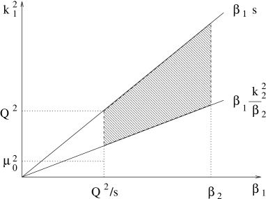
(a)   $\mu_{0}^{2}\,<\,\frac{k_{2}^{2}\,Q^{2}}{\beta_{2}\,s}$	(b)   $\mu_{0}^{2}\,>\,\frac{k_{2}^{2}\,Q^{2}}{\beta_{2}\,s}$

Figure 3: The integration domains for one rung: upper loop.

In the first case we have

$$\int_{Q^{2}/s}^{\beta_{2}}\,\frac{d\beta_{1}}{\beta_{1}}\,\int_{\beta_{1}\,k_{2}^{2}/\beta_{2}}^{s\,\beta_{1}}\,\frac{dk_{1}^{2}}{k_{1}^{2}}\,\,=\,\,\ln\frac{s\,\beta_{2}}{Q^{2}}\,\ln\frac{s\,\beta_{2}}{k_{2}^{2}},$$ (3.29)

whereas the second one leads to a sum of two contributions:

$$\int_{Q^{2}/s}^{\beta_{2}\,\mu_{0}^{2}/k_{2}^{2}}\,\frac{d\beta_{1}}{\beta_{1}}\,\int_{\mu_{0}^{2}}^{\beta_{1}\,s}\,\frac{dk_{1}^{2}}{k_{1}^{2}}\,\,+\,\,\int_{\beta_{2}\,\mu_{0}^{2}/k_{2}^{2}}^{\beta_{2}}\,\frac{d\beta_{1}}{\beta_{1}}\,\int_{\beta_{1}\,k_{2}^{2}/\beta_{2}}^{s\,\beta_{1}}\frac{dk_{1}^{2}}{k_{1}^{2}}$$

$$=\,\,\frac{1}{2}\,\left(\ln^{2}\frac{\beta_{2}\,s}{k_{2}^{2}}\,\,-\,\,\ln^{2}\frac{Q^{2}}{\mu_{0}^{2}}\right)\,\,+\,\,\ln\frac{k_{2}^{2}}{\mu_{0}^{2}}\,\ln\frac{\beta_{2}\,s}{k_{2}^{2}}\,.$$ (3.30)

For the remaining integrations over $\beta_{2}$ and $k_{2}^{2}$ (Fig. 4) we not only have to observe the distinction (3.27), (3.28), but also to return to the two cases defined in (2.12), (2.13).

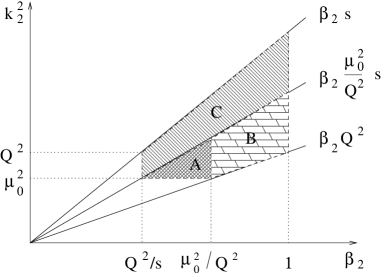
(a) $\mu_{0}^{2}\,<\,\frac{Q^{4}}{s}$	(b) $\mu_{0}^{2}\,>\,\frac{Q^{4}}{s}$

Figure 4: The integration domains for one rung: lower loop.

In the first case (i) we find (Fig. 4a) that the line $k_{2}^{2}\,=\,\beta_{2}\,Q^{2}$ always lies above the line $\beta_{2}\,\mu_{0}^{2}\,s/Q^{2}$ and $max(\beta_{2}\,Q^{2},\,\mu_{0}^{2})\,=\,\beta_{2}\,Q^{2}$. Therefore in the whole integration region (shaded area in Fig. 4a) we have $k_{2}^{2}/s\,>\,\beta_{2}\,\mu_{0}^{2}/Q^{2}$, and the first condition (3.27) is always fulfilled. This leads to

$$\int_{Q^{2}/s}^{1}\,\frac{d\beta_{2}}{\beta_{2}}\,\int_{\beta_{2}\,Q^{2}}^{\beta_{2}\,s}\,\frac{dk_{2}^{2}}{k_{2}^{2}}\,\ln\frac{\beta_{2}\,s}{Q^{2}}\,\ln\frac{\beta_{2}\,s}{k_{2}^{2}}\,=\,\frac{1}{4}\,\ln^{4}\,\frac{s}{Q^{2}}\,.$$ (3.31)

For the second case (ii) in (3.28) the situation is slightly more complicated (Fig. 4b): the region of integration (shaded area) consists of three pieces (denoted by A, B, and C). In C the first condition (3.27) holds, whereas in B and C the second one (3.28) is fulfilled. For region A the result is:

$$\int_{Q^{2}/s}^{\mu_{0}^{2}/Q^{2}}\,\frac{d\beta_{2}}{\beta_{2}}\,\int_{\mu_{0}^{2}}^{\beta_{2}\,s\,\mu_{0}^{2}/Q^{2}}\,\frac{dk_{2}^{2}}{k_{2}^{2}}\,\left(\frac{1}{2}\,\left(\ln^{2}\frac{\beta_{2}\,s}{k_{2}^{2}}\,-\,\ln^{2}\frac{Q^{2}}{\mu_{0}^{2}}\right)\,+\,\ln\frac{k_{2}^{2}}{\mu_{0}^{2}}\,\ln\frac{\beta_{2}\,s}{k_{2}^{2}}\right)$$

$$=\,\,\frac{1}{12}\,\ln^{4}\frac{s}{Q^{2}}\,-\,\frac{1}{2}\,\ln^{2}\frac{s}{Q^{2}}\,\ln^{2}\frac{Q^{2}}{\mu_{0}^{2}}\,+\,\frac{2}{3}\,\ln\frac{s}{Q^{2}}\,\ln^{3}\frac{Q^{2}}{\mu_{0}^{2}}\,-\,\frac{1}{4}\,\ln^{4}\frac{Q^{2}}{\mu_{0}^{2}}\,.$$ (3.32)

For region B we obtain:

$$\int_{\mu_{0}^{2}/Q^{2}}^{1}\,\frac{d\beta_{2}}{\beta_{2}}\,\int_{\beta_{2}\,Q^{2}}^{\beta_{2}\,s\,\mu_{0}^{2}/Q^{2}}\,\frac{dk_{2}^{2}}{k_{2}^{2}}\,\left(\frac{1}{2}\,\left(\ln^{2}\frac{\beta_{2}\,s}{k_{2}^{2}}\,-\,\ln^{2}\frac{Q^{2}}{\mu_{0}^{2}}\right)\,+\,\ln\frac{k_{2}^{2}}{\mu_{0}^{2}}\,\ln\frac{\beta_{2}\,s}{k_{2}^{2}}\right)$$

$$\,\,=\,\,\frac{1}{3}\,\ln^{3}\frac{s}{Q^{2}}\,\ln\frac{Q^{2}}{\mu_{0}^{2}}\,+\,\frac{1}{4}\,\ln^{2}\frac{s}{Q^{2}}\,\ln^{2}\frac{Q^{2}}{\mu_{0}^{2}}\,-\,\ln\frac{s}{Q^{2}}\,\ln^{3}\frac{Q^{2}}{\mu_{0}^{2}}\,+\,\frac{5}{12}\,\ln^{4}\frac{Q^{2}}{\mu_{0}^{2}}\,.$$ (3.33)

Finally, region C:

$$\int_{Q^{2}/s}^{1}\,\frac{d\beta_{2}}{\beta_{2}}\,\int_{\beta_{2}\,s\,\mu_{0}^{2}/Q^{2}}^{\beta_{2}\,s}\,\frac{dk_{2}^{2}}{k_{2}^{2}}\,\ln\frac{s\,\beta_{2}}{Q^{2}}\,\ln\frac{s\,\beta_{2}}{k_{2}^{2}}\,=\,\frac{1}{4}\,\ln^{2}\frac{s}{Q^{2}}\,\ln^{2}\frac{Q^{2}}{\mu_{0}^{2}}\,.$$ (3.34)

Adding up these three contributions we find

$$\frac{1}{12}\,\left(\ln^{4}\,\frac{s}{Q^{2}}\,+\,2\,\ln^{4}\frac{Q^{2}}{\mu_{0}^{2}}\right)\,+\,\frac{1}{3}\left(\ln^{3}\frac{s}{Q^{2}}\,\ln\frac{Q^{2}}{\mu_{0}^{2}}\,-\,\ln\frac{s}{Q^{2}}\,\ln^{3}\frac{Q^{2}}{\mu_{0}^{2}}\right)\,.$$ (3.35)

At the point $\mu_{0}^{2}\,=\,\frac{Q^{4}}{s}$ both results (3.31) and (3.35) coincide.

After the analysis of the one rung ladder diagram it is not difficult to see the general pattern and to derive an integral equation. The general diagram with $n$ rungs is illustrated in Fig. 2b. ¿From the trace expression in the numerator we obtain, for each rung, a factor $k_{i\perp}^{2}\,\lambda$, where the momentum factor cancels against one of the exchange propagators of the cell labeled by “i”. Following the strategy adopted for the one loop diagram and for the two loop case, we arrive at the $\alpha$ and $\beta$ integrals of the logarithmic type (2.10), with the ordering conditions

$$x\,<\,\alpha_{n}\,<\,\alpha_{n-1}\,...\,\alpha_{1}\,<\,1,\;\;\;\,\,\,\,\,\,\,\,\,\,\,\,x\,<\,\beta_{1}\,<\,\beta_{2}\,<\,...\,<\,\beta_{n-1}\,<\,\beta_{n}\,<\,1$$ (3.36)

and the additional constraints

$$\mu_{0}^{2}\,<\,s\,\alpha_{i}\,\beta_{i}\,=\,\vec{k}_{i}^{2}\,<\,s\,.$$ (3.37)

Translating to the variables $\beta_{i}$ and $k_{i}^{2}\,=\,\vec{k}_{i}^{2}$, the limits of integration of the $k_{i}^{2}$ become, in analogy with (3.26):

$$max(\beta_{n}\,Q^{2},\,\mu_{0}^{2})\,<\,k_{n}^{2}\,<\,\beta_{n}\,s,\;\,\,\,\,\,\,\,max(\frac{\beta_{n-1}\,k_{n}^{2}}{\beta_{n}},\,\mu_{0}^{2})\,<\,k_{n-1}^{2}\,<\,\beta_{n-1}\,s\;...\,,\,$$

$$max(\frac{\beta_{1}\,k_{2}^{2}}{\beta_{2}},\,\mu_{0}^{2})\,<\,k_{1}^{2}\,<\,\beta_{1}\,s\,.$$ (3.38)

Starting from cell 1 at the top, we now work our way down along the ladder. We first do the integrals of cell 1, keeping fixed the variables of all the other cells. In doing so, we are led to distinguish the two cases (3.27) and (3.28); the results are given in (3.29) and (3), which we denote by $A_{1}^{+}(\beta_{2},\,k_{2}^{2})$ and $A_{1}^{-}(\beta_{2},\,k_{2}^{2})$, resp. The following integration of cell 2 is done as described before: the only difference is that (2.12) and (2.13) are replaced by

$$I_{3}^{+}:\;\;\;\mu_{0}^{2}<\frac{Q^{2}k_{3}^{2}}{s\beta_{3}}\,;$$ (3.39)

$$I_{3}^{-}:\;\;\;\frac{Q^{2}k_{3}^{2}}{s\beta_{3}}<\mu_{0}^{2}\,.$$ (3.40)

As before, the ‘$+$’ region receives contributions only from the ‘$+$’ region (Fig.4a), whereas the ‘$-$’ region has contributions from both region A and B and from region C (Fig.4b). Denoting the results by $A_{2}^{+}(\beta_{3},\,k_{3}^{2})$ and $A_{2}^{-}(\beta_{3},\,k_{3}^{2})$, we have, symbolically,

$$A_{2}^{+}\,\,=\,\,K^{++}\,\,\otimes\,\,A_{1}^{+}$$ (3.41)

and

$$A_{2}^{-}\,\,=\,\,K^{-+}\,\,\otimes\,\,A_{1}^{+}\,\,+\,\,K^{--}\,\,\otimes\,\,A_{1}^{-}\,.$$ (3.42)

Note, in particular, that the evolution of $A^{+}$ decouples from $A^{-}$. The same pattern now repeats itself for the integration of cell 3 etc, and we can write down a recursion relation. Instead, we define $A^{\pm}(\beta,\,k^{2})\,=\,\sum_{n}\,A_{n}^{\pm}$ (where $A_{0}^{\pm}\,=\,1$) which satisfy the coupled integral equations (Fig. 5):

$$A^{+}(\beta,\,k^{2})\,=\,1\,+\,\lambda\,\int_{Q^{2}/s}^{\beta}\frac{d\beta^{\prime}}{\beta^{\prime}}\int_{\beta^{\prime}\,k^{2}/\beta}^{\beta^{\prime}\,s}\,\frac{dk^{{}^{\prime}2}}{k^{{}^{\prime}2}}\,A^{+}(\beta^{\prime},\,k^{{}^{\prime}2})$$ (3.43)

and

$$A^{-}(\beta,\,k^{2})\,\,=\,\,1\,+\,\lambda\,\int_{Q^{2}/s}^{\beta}\frac{d\beta^{\prime}}{\beta^{\prime}}\,\int_{\beta^{\prime}\,\mu_{0}^{2}/Q^{2}}^{\beta^{\prime}s}\,\frac{dk^{{}^{\prime}2}}{k^{{}^{\prime}2}}\,A^{+}(\beta^{\prime},\,k^{{}^{\prime}2})\,\,+$$

(3.44)

$$\lambda\int_{Q^{2}/s}^{\beta\,\mu_{0}^{2}/k^{2}}\frac{d\beta^{\prime}}{\beta^{\prime}}\int_{\mu_{0}^{2}}^{\beta^{\prime}\,\mu_{0}^{2}s/Q^{2}}\frac{dk^{{}^{\prime}2}}{k^{{}^{\prime}2}}\,A^{-}(\beta^{\prime},\,k^{{}^{\prime}2})\,+\,\lambda\,\int_{\beta\,\mu_{0}^{2}/k^{2}}^{\beta}\,\frac{d\beta^{\prime}}{\beta^{\prime}}\int_{\beta^{\prime}\,k^{2}/\beta}^{s\,\beta^{\prime}\,\mu_{0}^{2}/Q^{2}}\frac{dk^{{}^{\prime}2}}{k^{{}^{\prime}2}}\,A^{-}(\beta^{\prime},\,k^{{}^{\prime}2}).$$

Figure 5: The Bethe - Salpeter equation.

The first equation applies to the region $I_{A}^{+}$, the second one to $I_{A}^{-}$. They are defined by

$$I_{A}^{+}:\;\;\;\mu_{0}^{2}\,\,<\,\,\frac{Q^{2}\,k^{2}}{\beta\,s}$$ (3.45)

$$I_{A}^{-}:\;\;\;\frac{Q^{2}\,k^{2}}{\beta\,s}\,\,<\,\,\mu_{0}^{2}\,.$$ (3.46)

Finally, the amplitudes $T^{\pm}$ for the photon-photon scattering are obtained from $A$ by subtracting the terms $A_{0}^{\pm}\,=\,1$ and by putting $k^{2}\,=\,Q^{2}$ and $\beta\,=\,1$:

$$T^{\pm}(Q^{2},\,s)\,=\,\left[A^{\pm}(1,\,Q^{2})\,-\,1\right]\,\frac{\tau_{TT}}{\lambda}\,.$$ (3.47)

Note that in this limit the regions $I_{A}^{+}$, $I_{A}^{-}$ coincide with $I^{+}$ and $I^{-}$ in (2.12) and (2.13). The full scattering amplitude is obtained by adding the twisted (with respect to $s\leftrightarrow u$ crossing) fermion loop.

Before we finish this section we again briefly present the generalization to the case of unequal photon masses. With the main differences being the lower limits of the $\alpha$ and $\beta$ variables (analogous to (2.19)), the analysis for the one gluon rung and for the derivation of the integral equations can be done in exactly the same way as for the equal mass case; the final results for the integral equations are obtained from (3.43) and (3) by simply substituting $Q^{2}\to Q_{1}^{2}$:

$$A^{+}(\beta,k^{2})\,=\,1\,+\,\lambda\,\int_{Q_{1}^{2}/s}^{\beta}\frac{d\beta^{\prime}}{\beta^{\prime}}\,\int_{\beta^{\prime}\,k^{2}/\beta}^{\beta^{\prime}\,s}\,\frac{dk^{{}^{\prime}2}}{k^{{}^{\prime}2}}\,A^{+}(\beta^{\prime},\,k^{{}^{\prime}2})$$ (3.48)

and

$$A^{-}(\beta,\,k^{2})=1\,+\,\lambda\,\int_{Q_{1}^{2}/s}^{\beta}\frac{d\beta^{\prime}}{\beta^{\prime}}\int_{\beta^{\prime}\,\mu_{0}^{2}/Q_{1}^{2}}^{\beta^{\prime}\,s}\,\frac{dk^{{}^{\prime}2}}{k^{{}^{\prime}2}}A^{+}(\beta^{\prime},\,k^{{}^{\prime}2})\,+$$

$$\lambda \int_{Q_{1}^{2}/s}^{\beta\,\mu_{0}^{2}/k^{2}}\frac{d\beta^{\prime}}{\beta^{\prime}}\int_{\mu_{0}^{2}}^{\beta^{\prime}\,\mu_{0}^{2}\,s/Q_{1}^{2}}\frac{dk^{{}^{\prime}2}}{k^{{}^{\prime}2}}\,A^{-}(\beta^{\prime},\,k^{{}^{\prime}2})\,+\,\lambda\int_{\beta\,\mu_{0}^{2}/k^{2}}^{\beta}\frac{d\beta^{\prime}}{\beta^{\prime}}\int_{\beta^{\prime}\,k^{2}/\beta\,s}^{s\,\beta^{\prime}\,\mu_{0}^{2}/Q_{1}^{2}}\frac{dk^{{}^{\prime}2}}{k^{{}^{\prime}2}}\,A^{-}(\beta^{\prime},\,k^{{}^{\prime}2}).$$

The same replacement applies to the kinematic regions (3.45), (3.46). At the end we put $k^{2}\,=\,Q_{2}^{2}$ and $\beta\,=\,1$:

$$T^{\pm}(Q_{1}^{2},\,Q_{2}^{2},\,s)\,\,=\,\,\left[A^{\pm}(1,Q^{2}_{2})\,-\,1\right]\,\frac{\tau_{TT}}{\lambda}.$$ (3.50)

For the remainder of our paper we will stay with this general case of unequal photon masses.

4 Solution of the linear equations

The structure of the two equations, (3.48) and (3) defines our strategy: we first solve the equation for $A^{+}$, Eq. (3.48), and we then use the solution as an inhomogeneous term in the equation for $A^{-}$, Eq. (3).

4.1 Solution in the region $I_{A}^{+}$

In the region $I_{A}^{+}$ where Eq. (3.43) holds we define the new variables:

$$\xi\,=\,\ln(\beta\,s/k^{2})\,;\,\,\,\,\,\,\,\,\,\,\,\,\,\,\,\,\,\,\,\,\,\,\,\,\eta\,=\,\ln(\beta\,s/Q_{1}^{2})\,.$$

In these new variables the equation (3.43) can be rewritten

$$A^{+}(\xi,\,\eta)\,=\,1\,+\,\lambda\,\int^{\eta}_{0}\,d\bar{\eta}\,\int^{\xi}_{0}\,d\bar{\xi}\,A^{+}(\bar{\xi},\,\bar{\eta})\,.$$ (4.51)

When differentiated twice Eq. (4.51) reduces to

$$\frac{d^{2}A^{+}}{d\xi\,d\eta}\,\,=\,\,\lambda\,A^{+}\,.$$ (4.52)

A solution to Eq. (4.52) can be found in the following form

$$A^{+}(\xi,\,\eta)\,=\,\int_{0^{+}}\frac{dz}{2\,\pi\,i}\,\phi_{+}(z)\,e^{\,\eta\,z\,+\,\lambda\,\xi/z}\,,$$ (4.53)

with the integration path closed around the point $z\,=\,0$.

The function $\phi_{+}(z)$ is uniquely determined when (4.53) is substituted into Eq. (4.51). The result is

$$\phi_{+}(z)\,=\,\frac{1}{z},$$ (4.54)

and

$$A^{+}(\xi,\,\eta)\,=\,I_{0}\left(\sqrt{4\,\lambda\,\xi\,\eta}\right)\,.$$ (4.55)

4.2 Solution in the region $I_{A}^{-}$

In the region $I_{A}^{-}$ we have the integral equation (3) which couples the functions $A^{+}$ and $A^{-}$.

Again we define a new variable:

$$\xi^{\prime}\,=\,\xi\,-\,L_{0}\,;\,\,\,\,\,\,\,\,\,\,\,\,\,\,\,\,\,\,\,\,\,\,\,\,\,\,\,\,\,L_{0}\,=\,\ln(Q^{2}_{1}/\mu_{0}^{2})\,.$$

In the variables ($\xi^{\prime},\,\eta$) the equation (3) can be rewritten

$$A^{-}(\xi^{\prime},\,\eta)\,=\,1 + \lambda\,\int^{\eta}_{0}\,d\bar{\eta}\,\int_{-L_{0}}^{0}\,d\bar{\xi}\,A^{+}(\bar{\xi}^{\prime},\,\bar{\eta})$$ (4.56)

$$+ \lambda\,\int^{\xi^{\prime}}_{0}\,d\bar{\eta}\,\int^{\bar{\eta}}_{0}\,d\bar{\xi}^{\prime}\,A^{-}(\bar{\xi}^{\prime},\,\bar{\eta})\,+\,\lambda\,\int_{\xi^{\prime}}^{\eta}\,d\bar{\eta}\,\int^{\xi^{\prime}}_{0}\,d\bar{\xi}^{\prime}\,A^{-}(\bar{\xi}^{\prime},\,\bar{\eta})\,.$$

Note that, at $\xi^{\prime}=0$, $A^{-}(0,\eta)$ coincides with $A^{+}(L_{0},\eta)$: $0\,=\,\xi^{\prime}\,=\,\xi\,-\,L_{0}\,=\,\ln\frac{\beta\,s\,\mu_{0}^{2}}{k^{2}\,Q_{1}^{2}}$ denotes the point where the two regions $I_{A}^{+}$ and $I_{A}^{-}$ touch each other.

After double differentiation (4.56) reduces to

$$\frac{d^{2}A^{-}}{d\xi^{\prime}\,d\eta}\,=\lambda\,A^{-}\,.$$ (4.57)

For the solution we use the same ansatz as before:

$$A^{-}(\xi^{\prime},\,\eta)\,=\,\int_{0^{+}}\frac{dz}{2\,\pi\,i}\,\phi_{-}(z)\,e^{\,\eta\,z\,+\,\lambda\,\xi^{\prime}/z}\,,$$ (4.58)

with the integration path closed around $z=0$.

The function $\phi_{-}(z)$ is determined when (4.58) is substituted to Eq. (4.56). Note that the boundary condition $A^{-}(0,\,\eta)\,=\,A^{+}(L_{0},\,\eta)$ is respected by Eq. (4.56). The result (see Appendix A) is

$$\phi_{-}(z)\,=\,\frac{1}{z}\,e^{\lambda\,L_{0}/z}\,-\,\frac{z}{\lambda}\,e^{z\,L_{0}}$$ (4.59)

and

$$A^{-}(\xi^{\prime},\,\eta)\,=\,I_{0}\left(\sqrt{4\,\lambda\,(\xi^{\prime}\,+\,L_{0})\,\eta}\right)\,+\,\frac{\xi^{\prime}}{\eta+L_{0}}\,I_{2}\left(\sqrt{4\,\lambda\,\xi^{\prime}\,(\eta\,+\,L_{0})}\right).$$ (4.60)

4.3 Analyzing the solutions

Define

$$\omega_{0}\,=\,\sqrt{4\,\lambda}\,;\,\,\,\,\,\,\,\,\,\,\,\,\,\,\,\,\,\,\,\,\,\,\,\,\,\,\,\,\,\tilde{Q}^{2}=\sqrt{Q_{1}^{2}\,Q_{2}^{2}}\,.$$

The amplitude for $\gamma^{*}\,\gamma^{*}$ scattering is obtained using Eq. (3.47)

$$T^{+}\,=\,T(Q_{1}^{2},\,Q_{2}^{2},\,s)\,=\,\frac{4\;\tau_{TT}}{\omega_{0}^{2}}\,\left[I_{0}\left(\omega_{0}\,\sqrt{\ln\frac{s}{Q_{1}^{2}}\,\ln\frac{s}{Q_{2}^{2}}}\,\right)\,-\,1\right]\,\,\,\,\,\,\,\,\,\,\,if\,\,\,\,\mu_{0}^{2}\,<\,\tilde{Q}^{4}/s$$ (4.61)

and

$$T^{-} = T(Q_{1}^{2},\,Q_{2}^{2},\,s)\,=\,\frac{4\;\tau_{TT}}{\omega_{0}^{2}}\,\times$$ (4.62)

$$\left[I_{0}\left(\omega_{0}\,\sqrt{\ln\frac{s}{Q_{1}^{2}}\,\ln\frac{s}{Q_{2}^{2}}}\,\right)\,-\;1-\;\;\frac{\ln\frac{s\,\mu_{0}^{2}}{\tilde{Q}^{4}}}{\ln\frac{s}{\mu_{0}^{2}}}\,I_{2}\left(\omega_{0}\,\sqrt{\ln\frac{s\,\mu_{0}^{2}}{\tilde{Q}^{4}}\ln\frac{s}{\mu_{0}^{2}}}\right)\,\right]\,$$

$$\,\,\,\,\,\,\,\,\,\,\,\,\,\,\,\,\,\,\,\,\,\,\,\,\,\,\,\,\,\,\,\,\,\,\,\,\,\,\,\,\,\,\,\,\,\,\,\,\,\,\,\,\,\,\,\,\,\,\,\,\,\,\,\,\,\,\,\,\,\,\,\,\,\,\,\,\,\,\,\,\,\,\,\,\,\,\,\,\,\,\,\,\,\,\,\,\,\,\,\,\,\,\,\,\,\,\,\,\,\,\,\,\,\,\,\,\,\,\,\,\,\,\,\,\,\,\,if\,\,\,\,\mu_{0}^{2}\,>\,\tilde{Q}^{4}/s\,.$$

It is important to note that, although in the course of our derivation we seem to have lost the symmetry in $Q_{1}^{2}$ and $Q_{2}^{2}$, the final result of the amplitude is fully symmetric again. In particular, the second term depends upon $\tilde{Q}^{4}/s$ only. The amplitude $T^{-}$ reduces to $T^{+}$ when $\tilde{Q}^{4}/s=\mu_{0}^{2}$, i.e. when the dynamical infrared cutoff of the perturbative calculation reaches $\mu_{0}^{2}$, the limit of the nonperturbative infrared region.

Let us consider, in some more detail, the $s\rightarrow\infty$ asymptotics for the case $Q_{1}^{2}\,\simeq\,Q_{2}^{2}\gg\mu_{0}^{2}$. We take $s$ to be much larger than the $Q_{i}^{2}$, but still within the region $I^{+}$ (2.12):

$$1\ll s/\tilde{Q}^{2}\ll\tilde{Q}^{2}/\mu_{0}^{2}.$$ (4.63)

In this region the asymptotics is obtained from the asymptotic behavior of the Bessel function $I_{0}$

$$T^{+}(s\rightarrow\infty)\,=\,\frac{4\;\tau_{TT}}{\omega_{0}^{2}\,\,\sqrt{2\,\pi\,\omega_{0}\,\ln(s/\tilde{Q}^{2})}}\,\left(\frac{s}{\tilde{Q}^{2}}\right)^{\omega_{0}}\,,$$ (4.64)

and the result is entirely perturbative. When $s$ increases and eventually reaches the boarder line between $I^{+}$ and $I^{-}$:

$$s/\tilde{Q}^{2}=\tilde{Q}^{2}/\mu_{0}^{2}$$ (4.65)

we have to switch to $T^{-}$. With a further increase of $s$, initially, the second term in (3) is not large and we can use the expansion of the Bessel function $I_{2}$ for small arguments. In the asymptotic region

$$\tilde{Q}^{2}/\mu_{0}^{2}\ll s/\tilde{Q}^{2}$$ (4.66)

the arguments of both Bessel functions are large. Expanding in both $\frac{1}{\ln s/\tilde{Q}^{2}}$ and in the ratio $\frac{\ln\tilde{Q}^{2}/\mu_{0}^{2}}{\ln s/\tilde{Q}^{2}}$, we find that in (4.3) the leading terms of both Bessel function terms cancel against each other, and have to take into account first corrections. We obtain:

$$T^{-}(s\rightarrow\infty) = \frac{8\;\tau_{TT}}{\omega_{0}^{2}\,\sqrt{2\,\pi}\,(\omega_{0}\,\ln(s/\tilde{Q}^{2}))^{3/2}}\,\left(\frac{s}{\tilde{Q}^{2}}\right)^{\omega_{0}}\,\times$$

$$\left[1\,+\,\omega_{0}\,\ln\frac{\tilde{Q}^{2}}{\mu_{0}^{2}}\,+\,\frac{\omega_{0}^{2}}{4}\,\ln^{2}\frac{\tilde{Q}^{2}}{\mu_{0}^{2}}\,+\,O\left(\frac{\omega_{0}^{4}\,\ln^{4}\frac{\tilde{Q}^{2}}{\mu_{0}^{2}}}{\ln\frac{s}{\tilde{Q}^{2}}}\right)\right]\,.$$

It is interesting to compare (4.64) and (4.3): the power behavior in $s$ is the same in both regions. The difference lies in the preexponential factors: in the second region, we have a slightly stronger logarithmic suppression, and there is a logarithmic dependence upon the infrared scale $\mu_{0}^{2}$.

4.4 DIS at low $x$

Another case of interest is deep inelastic scattering on an almost real photon at very small $x$. This corresponds to the limit

$$\mu_{0}^{2}\approx Q_{2}^{2}\ll Q_{1}^{2}\ll s,$$ (4.68)

and only the region $I^{-}$ applies ($Q\equiv Q_{1}$):

$$T_{DIS}(Q^{2},\,s)\,=\,\left[I_{0}\left(\omega_{0}\,\sqrt{\ln\frac{s}{Q^{2}}\,\ln\frac{s}{\mu_{0}^{2}}}\,\right)\,-\,\frac{\ln\frac{s}{Q^{2}}}{\ln\frac{s}{\mu_{0}^{2}}}\,I_{2}\left(\omega_{0}\,\sqrt{\ln\frac{s}{Q^{2}}\ln\frac{s}{\mu_{0}^{2}}}\right)\,-\,1\right]\,\frac{4\;\tau_{TT}}{\omega_{0}^{2}}\,.$$

The Bjorken $x$ is defined in a standard way: $x\,\equiv\,Q^{2}/s$. The flavor nonsinglet photon structure function is related to $T_{DIS}$ via

$$F_{NS}^{\gamma}(x,Q^{2})\,=\,\frac{Q^{2}}{4\,\pi^{2}\,\alpha_{em}}\,\sigma^{\gamma^{*}\,\gamma}_{tot}\,=\,\frac{Q^{2}}{4\,\pi^{2}\,\alpha_{em}\,s}\,Im\,[T_{DIS}(Q^{2},\,s)]\,\simeq\,\frac{x}{4\,\pi\,\alpha_{em}}\,\frac{\partial\,T_{DIS}(Q^{2},\,s)}{\partial\ln\,s}\,.$$ (4.70)

Being aware of the fact that in the DIS limit ($Q^{2}_{2}\approx\mu_{0}^{2}$) the low $x$ saturation effects may be important [24] we will not discuss them here at all.

We can consider two different asymptotic limits. The first one is $\ln\,1/x\,\gg\,\ln\,Q^{2}/\mu_{0}^{2}\,\gg\,1$. In this limit the structure function becomes:

$$F_{NS}^{\gamma}(x,Q^{2})\,\simeq\,\left(\frac{1}{x}\right)^{-1\;+\;\omega_{0}}\,\,\frac{2\;\tau_{TT}\,(\,1\,+\,\omega_{0}\,\ln(Q^{2}/\mu_{0}^{2})/4\,)^{2}}{\alpha_{em}\,\omega_{0}^{2}\,\sqrt{2\,\pi\,\omega_{0}}\,\ln^{3/2}(1/x)}\,\left(\frac{Q^{2}}{\mu^{2}_{0}}\right)^{\omega_{0}/2}\,.$$ (4.71)

Eq. (4.71) gives the Regge limit of the flavor nonsinglet structure function. Up to the preexponential factor this result agrees with the behavior of the flavor nonsinglet proton structure function found in  [18].

Another asymptotic limit to be considered is $1\,\ll\,\ln\,(1/x)\,\ll\,\ln\,(Q^{2}/\mu_{0}^{2})$ leading to

$$F_{NS}^{\gamma}(x,Q^{2})\,\simeq\,x\,\,\frac{\tau_{TT}}{\alpha_{em}\,\pi\,\omega_{0}^{2}\,\sqrt{2\,\ln(1/x)\,\ln(Q^{2}/\mu_{0}^{2})}}\,e^{\,\omega_{0}\,\sqrt{\ln(1/x)\,\ln(Q^{2}/\mu_{0}^{2})}}\,.$$ (4.72)

Eq. (4.72) comes from the asymptotic expansion of the first term in (4.4). The second term is subleading in this limit. Eq. (4.72) corresponds to the double logarithmic limit of the DGLAP equation.

4.5 Scales

It is instructive to compare our results for the high energy behavior of quark-antiquark exchange in $\gamma^{*}\,\gamma^{*}$ scattering with those for gluon exchange, i.e. the LO BFKL Pomeron. For the latter it is well-known that, for sufficiently large photon virtualities and not too high energies, the internal transverse momenta are of the order of the photon virtualities and hence justify the use of perturbation theory (Fig. 6a). When energy grows, diffusion in $\ln k^{2}$ broadens the relevant region of internal transverse momenta, which has the shape of a “cigar”. Its mean size is of the order $\sqrt{\ln s}$ and eventually reaches the infrared cutoff $\mu_{0}^{2}$. From now on, the BFKL amplitude - although infrared finite - becomes sensitive to infrared physics, and some modification due to nonperturbative physics has to be included.

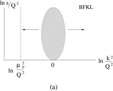
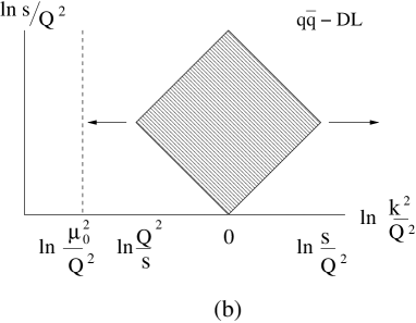
Figure 6: Energy dependence of the region of integration in a) BFKL and b) quark ladder.

With the results of our analysis we now can make an analogous statement about quark-antiquark exchange. Since internal transverse momenta range between $max(Q^{4}/s,\,\mu_{0}^{2})\,<\,k^{2}\,<\,s$ or, equivalently

$$max(-\,\ln s/Q^{2},\,\ln\,\mu_{0}^{2}/Q^{2})\,\,<\,\,\ln\,k^{2}/Q^{2}\,\,<\,\,\ln\,s/Q^{2}\,,$$ (4.73)

there is, for not too large energies, again, a limited region where transverse momenta stay above the infrared scale, and the use of perturbative QCD is justified. With increasing energy, the $k^{2}$-region expands and eventually hits the infrared cutoff $\mu_{0}^{2}$. From now on the high energy behavior starts to depend upon infrared physics and requires suitable modifications.

In order to understand, in the fermion case, the region of internal integration in more detail, let us first return to our amplitude, $A^{+}$ (illustrated in Fig.5). It satisfies the two dimensional wave equation (4.52). It is instructive to introduce the new variables

$$t\,=\,\frac{1}{2}\,(\xi\,+\,\eta)\,=\,\ln\frac{\beta s}{\sqrt{k^{2}Q^{2}}}\,;\,\,\,\,\,\,\,\,\,\,\,\,\,\,\,\,\,\,\,\,\,\,\,\,\,\,\,\,z\,=\,\frac{1}{2}\,(\eta\,-\,\xi)\,=\,\frac{1}{2}\,\ln\frac{k^{2}}{Q^{2}},$$ (4.74)

which leads to the two-dimensional Klein-Gordon equation:

$$\left(\frac{\partial^{2}}{\partial t^{2}}\,-\,\frac{\partial^{2}}{\partial z^{2}}\,-\,4\,\lambda\right)\,\,A^{+}\;=\;0$$ (4.75)

(here $i\sqrt{4\,\lambda}$ plays the role of the mass).

Figure 7: Light cone variables for the wave equation.

As seen from (4.51), our amplitude satisfies the boundary condition $A^{+}(0,\,0)\,=\,1$, and its normal derivatives vanish on the ‘light cone’ $\xi\,=\,0$ or $\eta\,=\,0$. Let us illustrate this in Fig. 5: the upper end of the ladder we associate with the values $\beta\,\approx\,Q^{2}/s$ and $k^{2}\,\approx\,Q^{2}$, which translates into $\xi\,=\,\eta\,=\,0$ or $t\,=\,z\,=\,0$. At the lower end, when coupling to the external photon, we put $\beta\,=\,1$, $k^{2}\,=\,Q^{2}$, which is equivalent to $\xi\,=\,\eta\,=\,\ln\,s/Q^{2}$ or $t\,=\,\ln\,s/Q^{2}$,   $z\,=\,0$. Correspondingly, in Fig.7 the $t$-axis points downwards: our ladder diagrams for $\gamma^{*}\,\gamma^{*}$ describe the evolution (in $t$) from the initial point $(t_{i},\,z_{i})\,=\,(0,\,0)$ (upper photon) to the final point $(t_{f},\,z_{f})\,=\,(\ln\,s/Q^{2},\,0)$ (lower photon). As seen from (4.51), all paths lie in the region of positive $\xi$ and $\eta$, i.e. they stay inside the square described by $0\,<\,\xi\,<\,\xi_{f}\,=\,\ln\,s/Q^{2}$,   $0\,<\,\eta\,<\,\eta_{f}\,=\,\ln\,s/Q^{2}$. Note the width in $z$: it starts from zero, increases up to its maximal value $\ln\,s/Q^{2}$, and finally it shrinks down to zero again.

Let us confront this with the BFKL Pomeron: in Fig.6b we have, once more, drawn the square which illustrates the internal region of integration. Apart from the difference in shape (“diamond” versus “cigar”), the most notable difference is the width in $\ln k^{2}$. In the fermion case it grows proportional to $\ln\,s/Q^{2}$, i.e stronger than in the BFKL case where $\ln\,k^{2}$ grows as $\sqrt{\ln\,s/Q^{2}}$: the BFKL diffusion is replaced by a linear growth in the $z$-direction. Also the definition of ‘internal rapidity’ is different: in the BFKL case the vertical axis can be labeled simply by $\ln\,1/\beta$, whereas in the fermion case our variable is $t\,=\,\ln\,(\beta\,s/\sqrt{k^{2}\,Q^{2}})$ (in both cases, the total length grows proportional to $\ln s$).

5 InfraRed Evolution Equation

In this section we rederive our previous result from the IREE. We define the partial wave through the ansatz::

$$T(Q_{1}^{2},\,Q_{2}^{2},\,s)\,=\,\int\frac{d\omega}{2\,\pi\,i}\,\left(\frac{s}{\tilde{\mu}^{2}}\right)^{\omega}\,\tilde{T}(Q_{1}^{2}/\tilde{\mu}^{2},\,Q_{2}^{2}/\tilde{\mu}^{2},\,\omega)\,.$$ (5.76)

For a more detailed description of the method we refer the reader to the original work [17] as well as to some applications in Ref. [15, 18, 19, 25]. The scale $\tilde{\mu}$ is introduced as an auxiliary infrared cutoff parameter, which, a priori, does not have to coincide with the infrared cutoff scale of nonperturbative physics, $\mu_{0}$. Before applying the IREE formalism to $\gamma^{*}\,\gamma^{*}$ scattering, we have to discuss its applicability. Based upon our previous analysis, we have to distinguish between two cases. For any t-channel quark line we have the condition that $\mu_{0}^{2}\,<\,s\,\alpha\,\beta\,=\,k^{2}$ which, in the derivation of the IREE, will be replaced by $\tilde{\mu}^{2}\,<\,s\,\alpha\,\beta\,=\,k^{2}$. On the other hand, we have the constraints that $Q_{1}^{2}/s<\beta$, and $Q_{2}^{2}/s<\alpha$. Combining these conditions we have $max(\tilde{\mu}^{2},\,Q_{1}^{2}\,Q_{2}^{2}/s)\,<\,s\,\alpha\,\beta\,=\,k^{2}$, and this distinction (after identifying the auxiliary parameter $\tilde{\mu}$ with the physical infrared cutoff $\mu_{0}$) leads to the the two regions, $I^{+}$ and $I^{-}$. In the latter case, all internal transverse momenta are cutoff by $\tilde{\mu}$, and this is the case where the IREE directly applies. In the former case, the internal momenta do not reach the value $\tilde{\mu}$, i.e. the amplitude is independent of $\tilde{\mu}$. This case, therefore, has to be studied separately.

Let us begin with the genuine IREE region, $Q_{1}^{2}\,Q_{2}^{2}/s\,<\,\tilde{\mu}^{2}$. The IREE for the amplitude $T$ is obtained by differentiating (5.76) with respect to $\ln\tilde{\mu}^{2}$. In $\omega$ space this essentially corresponds to cutting of the diagram on two parts (see Fig 8).

Figure 8: The IRRE for $\gamma^{*}\,\gamma^{*}$.

The equation reads

$$\omega\,\tilde{T}^{-}\,\,+\,\,\frac{\partial\tilde{T}^{-}}{\partial y_{1}}\,\,+\,\,\frac{\partial\tilde{T}^{-}}{\partial y_{2}}\,\,=\,\,2\,N_{c}\,F_{nc}\,\,\frac{F(\omega,y_{1})\,\,F(\omega,y_{2})}{8\,\pi^{2}}$$ (5.77)

with $y_{1,2}\,\equiv\,\ln(Q_{1,2}^{2}/\tilde{\mu}^{2})$,

$$F(\omega,\,y)\,=\,\frac{C_{0}}{g^{2}\,C_{F}}\,f_{0}(\omega)\,e^{\,-(\omega-f_{0}/8\pi^{2})\,y}\,\,\,\,\,\,\,\,\,\,\,\,\,\,\,\,for\,\,\,\,\,\,\,\,y\geq 0\,,$$ (5.78)

and $C_{0}\,=\,4\,\pi\,\alpha_{em}\,\epsilon(A)\,\cdot\,\epsilon(A^{\prime})$.

The function $f_{0}$ was introduced in Ref. [17]

$$f_{0}(\omega)\,=\,4\,\pi^{2}\,(\omega\,-\,\sqrt{\omega^{2}-\omega_{0}^{2}})$$ (5.79)

with the property:

$$f_{0}\,(\omega\,-\,\frac{f_{0}}{8\,\pi^{2}})\,=\,2\,\pi^{2}\,\omega_{0}^{2}\,.$$ (5.80)

The function $F(\omega,\,y)$ is a solution of the IREE for a quark-photon amplitude [17, 18]. The coefficient $C_{0}$ contains information about coupling of the photon to the ladder. Note the appearance in (5.77) of the factor $2\,N_{c}\,F_{nc}$ which incorporates a proper normalization for the case of $\gamma^{*}\,\gamma^{*}$.

We should impose boundary conditions for the case when only one photon is (nearly) on shell. For the boundary $y_{1}\,\geq\,y_{2}\,=\,0$ it reads:

$$\omega\,\tilde{T}^{-}(y_{1},\,y_{2}\,=\,0)\,\,+\,\,\frac{\partial\tilde{T}^{-}(y_{1},\,y_{2}\,=\,0)}{\partial y_{1}}\,\,=\,\,2\,N_{c}\,F_{nc}\,\frac{F(\omega,y_{1})\,F(\omega,y_{2}\,=\,0)}{8\,\pi^{2}}\,.$$ (5.81)

A similar condition is imposed at the second boundary $y_{2}\,\geq\,y_{1}\,=\,0$. When both photons are (nearly) on shell we have an additional equation

$$\omega\,\tilde{T}^{-}(y_{1}\,=\,y_{2}\,=\,0)\,\,=\,\,2\,N_{c}\,F_{nc}\,\frac{F^{2}(\omega,y\,=\,0)}{8\,\pi^{2}}.$$ (5.82)

We will find now a solution of Eq. (5.77) with the boundary conditions (5.81) and (5.82). Note that the solution to be found is unique.

A general solution of the inhomogeneous equation (5.77) can be found as a sum of a particular solution ($\tilde{T}_{ps}$) and a solution of the homogeneous equation ($\tilde{T}_{he}$), such that $\tilde{T}^{-}\,=\,\tilde{T}_{ps}\,+\,\tilde{T}_{he}$. We will search for $\tilde{T}_{ps}$ using the following ansatz, which is motivated by the right hand side of (5.77):

$$\tilde{T}_{ps}(\omega)\,=\,\tilde{T}_{ps}^{0}(\omega)\,e^{\,-(\omega\,-\,f_{0}/8\pi^{2})\,(y_{1}\,+\,y_{2})}\,.$$ (5.83)

Substituting it to (5.77) we find $\tilde{T}_{ps}^{0}(\omega)$:

$$\tilde{T}_{ps}(\omega)\,=\,-\,\kappa\frac{f_{0}^{2}}{\omega\,-\,f_{0}/4\,\pi^{2}}\,e^{\,-(\,\omega\,-\,f_{0}/8\pi^{2})\,(y_{1}\,+\,y_{2})}$$ (5.84)

with

$$\kappa\,=\,\frac{C_{0}(A)\,C_{0}(B)\,2\,N_{c}\,F_{nc}}{8\,\pi^{2}\,g^{4}\,C_{F}^{2}}\,=\,\frac{\tau_{TT}}{g^{4}\,C_{F}^{2}}\,=\,\frac{\tau_{TT}}{4\,\pi^{4}\,\omega_{0}^{4}}\,.$$ (5.85)

Our goal now is to find $\tilde{T}_{he}$ which satisfies the homogeneous version of Eq.(5.77). Define two new variables: $w\,=\,y_{1}\,+\,y_{2}$ and $u\,=\,y_{1}\,-\,y_{2}$. Then

$$\omega\,\tilde{T}_{he}(\omega)\,+\,2\,\frac{\partial\tilde{T}_{he}}{\partial w}\,=\,0$$ (5.86)

with the solution

$$\tilde{T}_{he}(\omega,u,w)\,=\,\tilde{T}^{0}_{he}(\omega,\,u)\,e^{-\omega\,w/2}\,=\,\tilde{T}^{0}_{he}(\omega,\,y_{1}\,-\,y_{2})\,e^{-\omega\,(y_{1}\,+\,y_{2})/2}.$$ (5.87)

The boundary conditions (5.81) and (5.82) will be used in order to find $\tilde{T}^{0}_{he}$. When $\tilde{T}^{-}\,=\,\tilde{T}_{ps}\,+\,\tilde{T}_{he}$ is substituted in Eq. (5.81) we get ($y_{2}=0$)

$$\frac{\omega}{2}\,\tilde{T}^{0}_{he}\,+\,\frac{\partial\tilde{T}^{0}_{he}}{\partial y_{1}}\,=\,\kappa\,\frac{f_{0}^{2}\,(\omega\,-\,f_{0}/8\,\pi^{2})}{\omega\,-\,f_{0}/4\,\pi^{2}}\,\,e^{\,-\,(\omega\,-\,f_{0}/4\,\pi^{2})\,y_{1}/2}\,.$$ (5.88)

With the help of (5.80) the rhs can be simplified:

$$\frac{\omega}{2}\,\tilde{T}^{0}_{he}\,+\,\frac{\partial\tilde{T}^{0}_{he}}{\partial y_{1}}\,=\kappa\,\frac{2\,\pi^{2}\,\omega_{0}^{2}\,f_{0}}{\omega\,-\,f_{0}/4\,\pi^{2}}\,\,e^{\,-\,(\omega\,-\,f_{0}/4\,\pi^{2})\,y_{1}/2}\,.$$ (5.89)

Eq. (5.88) has a solution which, again, is given by a sum of a particular solution ($R_{ps}$) and a solution of the homogeneous equation ($R_{he}$), such that $\tilde{T}^{0}_{he}\,=\,R_{ps}\,+\,R_{he}$. The particular solution is

$$R_{ps}(\omega,\,y_{1})\,=\,\kappa\,\frac{16\,\pi^{4}\,\omega_{0}^{2}}{\omega\,-\,f_{0}/4\,\pi^{2}}\,\,e^{\,-\,(\omega\,-\,f_{0}/4\,\pi^{2})\,y_{1}/2}\,,$$ (5.90)

while the solution of the homogeneous equation is

$$R_{he}(\omega,\,y_{1})\,=\,R_{he}^{0}\,e^{\,-\omega\,y_{1}/2}\,.$$ (5.91)

Finally we use the boundary condition (5.82) in order to determine $R_{he}^{0}$:

$$R_{he}^{0}(\omega)\,=\,-\kappa\,\frac{16\,\pi^{4}\,\omega_{0}^{2}}{\omega}\,.$$ (5.92)

Combining all the results together we find the desired solution:

$$\tilde{T}^{-}(\omega)\, = \,-\,\kappa\,\frac{f_{0}^{2}}{\omega\,-\,f_{0}/4\,\pi^{2}}\,e^{\,-(\omega\,-\,f_{0}/8\pi^{2})\,(y_{1}\,+\,y_{2})}\,\,\,+$$

$$16\,\pi^{4}\,\kappa\,\omega_{0}^{2}\,e^{\,-\,y_{1}\,\omega}\,\left[\,\frac{1}{(\omega\,-\,f_{0}/4\,\pi^{2})}\,e^{\,-(y_{2}\,-\,y_{1})\,f_{0}/8\,\pi^{2}}\,-\,\frac{1}{\omega}\,\right]\,,$$

which we can also write as

$$\tilde{T}^{-}(\omega) = -\,16\,\pi^{4}\,\kappa\,\frac{(\omega\,-\,\sqrt{\omega^{2}\,-\,\omega_{0}^{2}})^{2}}{\sqrt{\omega^{2}\,-\,\omega_{0}^{2}}}\,e^{\,-(\omega\,-\,f_{0}/8\,\pi^{2})\,(y_{1}\,+\,y_{2})}$$ (5.94)

$$+ 16\,\pi^{4}\,\kappa\,\omega_{0}^{2}\,\left[\frac{e^{\,-\,\omega(y_{1}\,+\,y_{2})/2}\,\,e^{\,(y_{2}\,-\,y_{1})\sqrt{\omega^{2}\,-\,\omega_{0}^{2}}/2}}{\sqrt{\omega^{2}\,-\,\omega_{0}^{2}}}\,-\,\frac{e^{\,-\,y_{1}\,\omega}}{\omega}\right].$$

In (5) and (5.94), the first term on the rhs is the particular solution of Eq. (5.77), whereas the second term is a solution of the homogeneous equation. Since we used the boundary condition (5.81), the solution (5) (or (5.94)) is valid for $y_{1}\,>\,y_{2}$. Would we have started with the boundary conditions at $y_{1}=0$, we would have ended up with (5) or (5.94), but with $y_{1}$ and $y_{2}$ being interchanged.

At first sight, the distinction between the two cases $y_{1}\,<\,y_{2}$ and $y_{2}\,<\,y_{1}$ might look somewhat strange. Returning with our result into (5.76), putting $\tilde{\mu}^{2}\,=\,\mu_{0}^{2}$, we reproduce exactly the expression (4.62) for the amplitude $T^{-}$. It is not difficult to identify (after integration over $\omega$) the first term on the rhs of (5.94) with the second term on the rhs of (4.62) (the Bessel function $I_{2}$), whereas the “nonsymmetric” second term equals $I_{0}\,-\,1$. The final result is fully symmetric with respect to $y_{1}\,\leftrightarrow\,y_{2}$ interchange. The apparent puzzle is resolved because of the two-sheeted structure of the $\omega$ plane for the partial wave representation of the Bessel function $I_{0}$ (see Appendix B).

Finally, we return to the other region, $\tilde{\mu}^{2}\,<\,Q_{1}^{2}\,Q_{2}^{2}/s$. As we have argued above, in this region the amplitude does not depend upon $\tilde{\mu}^{2}$. Starting from the ansatz (5.76), we have to require that the total derivative with respect to $\tilde{\mu}^{2}$ vanishes, i.e.

$$\omega\,\tilde{T}^{+}\,+\,\frac{\partial\tilde{T}^{+}}{\partial y_{1}}\,\,+\,\,\frac{\partial\tilde{T}^{+}}{\partial y_{2}}\,\,=\,\,0\,.$$ (5.95)

A solution to this equation has to be of the form (5.87), where the dependence upon the difference $y_{1}\,-\,y_{2}$ has to be fixed by boundary conditions. We require that, for $\tilde{\mu}^{2}\,=\,Q_{1}^{2}\,Q_{2}^{2}/s$ the solution matches the solution (5.94), found for the other region, $I^{-}$. Since, on the rhs of (5.94), the first term after integration over $\omega$ is proportional to the Bessel function $I_{2}(\omega_{0}\,\sqrt{\ln(s\tilde{\mu}^{2}/\tilde{Q}^{2})\,\ln(s/\tilde{\mu}^{2})})$ and vanishes for $s\tilde{\mu}^{2}/\tilde{Q}^{2}\,=\,1$, we are left with the second term only and our result is

$$\tilde{T}^{+}(\omega)\,=\,16\,\pi^{4}\,\kappa\,\omega_{0}^{2}\,\left[\frac{e^{\,-\,\omega\,(y_{1}\,+\,y_{2})/2}\,\,e^{\,(y_{2}\,-\,y_{1})\,\sqrt{\omega^{2}\,-\,\omega_{0}^{2}}/2}}{\sqrt{\omega^{2}\,-\,\omega_{0}^{2}}}\,-\,\frac{e^{\,-\,y_{1}\,\omega}}{\omega}\right].$$ (5.96)

After integration over $\omega$, this becomes $I_{0}\,-\,1$, in agreement with (4.61).

In summary, we have been able to derive, within the IREE approach, both our solutions $T^{-}$ and $T^{+}$. This result allows for the possibility of studying also non-ladder diagrams which appear in odd signature exchange amplitudes.

6 Reggeon Green’s function

A third method of describing the double logarithmic high energy behavior of quark-antiquark exchange has been developed in Ref. [21]. Kirschner has shown that the double logarithmic situation can be described in the same way as the BFKL Pomeron, namely by a two-reggeon Green’s function with a kernel which is conformal invariant and holomorphic separable. In particular, in the integral equation of the reggeon Green’s function the transverse momentum integration has no explicit infrared or ultraviolet cutoff; therefore it has to be compared with our result for $\mu_{0}=0$. In the following we will show that, starting from Kirschner’s Green’s function, we arrive at the same result as in section 4.

The reggeon Green function in Ref. [21] has been obtained by deriving and solving a linear BFKL-type equation for the quark exchange amplitude [20]. The Green function has the form

$$G(k_{\perp}\,,\,\bar{k}_{\perp}\,,\,\omega)\,=\,\frac{1}{2\,\pi^{2}}\int_{-\infty}^{\infty}d\,\nu\,\sum_{n=-\infty}^{\infty}\frac{|k_{\perp}^{2}|^{-\,1\,+\,i\,\nu}\left(\frac{k_{\perp}}{|k_{\perp}|}\right)^{n}\,|\bar{k}_{\perp}^{2}|^{-\,1\,-\,i\,\nu}\left(\frac{\bar{k}_{\perp}}{|\bar{k}_{\perp}|}\right)^{-n}}{\omega\,-\,\omega_{0}^{2}\,\Omega(\omega,\,\nu,\,n)/4}$$ (6.97)

with

$$\Omega(\omega,\,\nu,\,n)\,=\,4\,\psi(1)\,-\,\psi(-\,i\,\nu\,+\,\frac{|n|}{2}\,+\,\frac{\omega}{2})\,-\,\psi(i\,\nu\,+\,\frac{|n|}{2}\,+\,\frac{\omega}{2})\,-\,$$

$$\psi(1\,-\,i\,\nu\,-\,\frac{|n|}{2}\,+\,\frac{\omega}{2})\,-\,\psi(1\,+\,i\,\nu\,-\,\frac{|n|}{2}\,+\,\frac{\omega}{2})$$ (6.98)

and $\psi(z)\,=\,\frac{d}{d\,z}\,\ln\Gamma(z)$. The function $G$ is normalized such that at the Born level it equals $G_{0}=\frac{1}{\omega\,k_{\perp}^{2}}\,\delta^{2}(k_{\perp}\,-\,\bar{k}_{\perp})$, which is a propagator of two quark lines.

At high energies the leading contribution comes from $n\,=\,0$. After expansion of $\Omega$ for small values of $\omega$ and $\nu$ the Green functions reduces to

$$G(k_{\perp}\,,\,\bar{k}_{\perp}\,,\,\omega)\,=\,\frac{1}{2\,\pi^{2}}\frac{1}{k_{\perp}^{2}\,\bar{k}_{\perp}^{2}}\int_{-\infty}^{\infty}d\,\nu\,\frac{\omega^{2}\,+\,4\,\nu^{2}}{\omega\,(\omega^{2}\,-\,\omega_{0}^{2}\,+\,4\,\nu^{2})}\,\left(\frac{k^{2}_{\perp}}{\bar{k}_{\perp}^{2}}\right)^{i\,\nu}$$ (6.99)

The $\gamma^{*}\,\gamma^{*}$ scattering amplitude can be obtained from $G$ by integrating over momenta $k$ in the low and upper blocks in Fig. 9. Note that the propagators of the t-channel quarks ($1/k^{2}$) are already included in $G$. In Ref. [21] they were assumed to be purely transverse implying that

$$\alpha\,\beta\,s\,\ll\,k_{\perp}^{2}\,\,\,\,\,\,\,\,\,\,\,\,\,\,\,\,\,\,\,\,\,and\,\,\,\,\,\,\,\,\,\,\,\,\,\,\,\,\,\,\,\,\bar{\alpha}\,\bar{\beta}\,s\,\ll\,\bar{k}_{\perp}^{2}\,.$$ (6.100)

The $\bar{\alpha}$ and $\beta$ integrations pick up the poles of the $s$-channel quark propagators. The only trace of these integrations is in the ordering (3) in $\bar{k}^{2}/\bar{\beta}$ (and in $k^{2}/\alpha$). This ordering leads to the following limits for $\beta$ and $\bar{\alpha}$:

$$\,\alpha_{max}\,=\,min\{1\,,k_{\perp}^{2}/Q_{2}^{2}\}\,\,\,\,\,\,\,\,\,\,\,\,\,\,\,\,\,\,\,\,\,\,\,\,\,\,\bar{\beta}_{max}\,=\,min\{1\,,\bar{k}_{\perp}^{2}/Q_{1}^{2}\}.$$

The scattering amplitude has the form

$$T_{G}^{\gamma^{*}\,\gamma^{*}}(Q_{1}^{2},\,Q^{2}_{2},\,s)\,=\,\tau_{TT}\,\int d^{2}\,k_{\perp}\int_{0}^{\alpha_{max}}\frac{d\alpha}{\alpha}\int d^{2}\,\bar{k}_{\perp}\int_{0}^{\bar{\beta}_{max}}\frac{d\bar{\beta}}{\bar{\beta}}$$

$$\times\,\int\frac{d\,\omega}{2\,\pi\,i}\,\left(\frac{\alpha\,\bar{\beta}\,s}{|k_{\perp}|\,|\bar{k}_{\perp}|}\right)^{\omega}\,\omega\,G(k_{\perp},\,\bar{k}_{\perp},\,\omega)\,.$$ (6.101)

The overall coefficient $\tau_{TT}$ as well as the factor $\omega$ in front of $G$ account for the proper normalization and can be deduced using the Born approximation. Note that, following the derivation of $G$ in [21], we assume that any potential infrared and ultraviolet divergences stemming from the $k_{\perp}$ integrations are regularized by the $\omega$ dependent factor. This is why the $\omega$ integration should be done only after the $k_{\perp}$ integrations are performed.

After the $\alpha$ and $\bar{\beta}$ integrations we obtain:

$$T_{G}^{\gamma^{*}\,\gamma^{*}}\,=\,\tau_{TT}\,\int d^{2}\,k_{\perp}\int d^{2}\,\bar{k}_{\perp}\int\frac{d\,\omega}{2\,\pi\,i\,\omega}\,\left(\frac{\alpha_{max}\,\bar{\beta}_{max}\,s}{|k_{\perp}|\,|\bar{k}_{\perp}|}\right)^{\omega}\,G(k_{\perp},\,\bar{k}_{\perp},\,\omega)\,.$$ (6.102)

It is worth to notice that the $\gamma^{*}\,\gamma^{*}$ scattering amplitude can be brought to the form in which $G$ is sandwiched between the photon impact factors:

$$T_{G}^{\gamma^{*}\,\gamma^{*}}\,=\,N_{c}\,F_{nc}\,\int\frac{d^{2}\,k_{\perp}}{2\,\pi}\int\frac{d^{2}\,\bar{k}_{\perp}}{2\,\pi}\int\frac{d\,\omega}{2\,\pi\,i\,\omega}\,\left(\frac{s}{|k_{\perp}|\,|\bar{k}_{\perp}|}\right)^{\omega}\,$$

(6.103)

$$\times\,\Phi(Q_{1}^{2},\,k_{\perp}^{2},\,\omega)\,\,G(k_{\perp},\,\bar{k}_{\perp},\,\omega)\,\,\Phi(Q_{2}^{2},\,\bar{k}_{\perp}^{2},\,\omega).$$

The photon impact factor has the form

$$\Phi(Q^{2},\,k_{\perp}^{2},\,\omega)\,=\,C_{0}\,\left[\,\left(\frac{k_{\perp}^{2}}{Q^{2}}\right)^{\omega}\,\,\Theta\left(1\,-\,\frac{k_{\perp}^{2}}{Q^{2}}\right)\,\,+\,\,\Theta\left(\frac{k_{\perp}^{2}}{Q^{2}}\,-\,1\right)\,\right]\,.$$ (6.104)

with $C_{0}$ defined in the previous section. Integrating in (6.102) over $k_{\perp}\,,\bar{k}_{\perp}$ we get

$$T_{G}^{\gamma^{*}\,\gamma^{*}}\,=\,\frac{8\,\tau_{TT}}{\pi}\,\int\frac{d\,\omega}{2\,\pi\,i}\,\int_{-\infty}^{\infty}d\,\nu\,\frac{1}{(\omega^{2}\,+\,4\,\nu^{2})\,(\omega^{2}\,-\,\omega_{0}^{2}\,+\,4\,\nu^{2})}\,\left(\frac{s}{\tilde{Q}^{2}}\right)^{\omega}\,\left(\frac{Q_{1}^{2}}{Q_{2}^{2}}\right)^{i\,\nu}\,.$$ (6.105)

The $\nu$ integration leads to

$$T_{G}^{\gamma^{*}\,\gamma^{*}}\,=\,\frac{4\,\tau_{TT}}{\omega_{0}^{2}}\,\int\frac{d\,\omega}{2\,\pi\,i}\,\left(\frac{s}{\tilde{Q}^{2}}\right)^{\omega}\,\left[\,\left(\frac{Q_{1}^{2}}{Q_{2}^{2}}\right)^{-\sqrt{\omega^{2}-\omega_{0}^{2}}/2}\,\frac{1}{\sqrt{\omega^{2}\,-\,\omega_{0}^{2}}}\,-\,\frac{1}{\omega}\,\left(\frac{Q_{1}^{2}}{Q_{2}^{2}}\right)^{-\omega/2}\,\right]\,.$$ (6.106)

Finally, after the $\omega$ integration we arrive at:

$$T_{G}^{\gamma^{*}\,\gamma^{*}}\,=\,\frac{4\,\tau_{TT}}{\omega_{0}^{2}}\,\left[\,I_{0}\,\left(\omega_{0}\,\sqrt{\ln\frac{s}{Q_{1}^{2}}\,\ln\frac{s}{Q_{2}^{2}}}\,\right)\,\,-\,\,1\,\right]\,.$$ (6.107)

The expression (6.107) coincides exactly with the amplitude $T^{+}$ (4.61), with the restriction $\mu_{0}^{2}<Q^{4}/s$ being removed. Formally we can say that the Green’s function approach should be compared to our previous treatment (in particular, the linear equation in section 4) with $\mu_{0}^{2}=0$ being put to zero. A striking difference between the two treatments lies in the integration over transverse momenta. From the discussion in section 4 it follows that all transverse momenta inside the ladder lie in the region $Q^{4}/s\,<\,k^{2}\,<\,s$. In the integral equation for the reggeon Green’s function [21], on the other hand, the Regge energy factor $\left(s/k_{\perp}k_{\perp}^{\prime}\right)^{\omega}$ serves as a regulator, and the transverse momentum integration can be extended down to zero and up to infinity.

Figure 9: $\gamma^{*}\,\gamma^{*}$ via reggeon Green function.

An easy way to see how this works is the following. Return to our two-loop integral in section 3 and compare the lower cell, $k_{2}$, with the $\bar{k}$ integration in (6.101). The integration region is illustrated in Fig. 4a: interchanging the order of integration over $\beta_{2}$, $k_{2}$, we see that the $k_{2}$ integration goes from $Q^{4}/s$ to $s$ and splits into two pieces. For $Q^{4}/s\,<\,k_{2}^{2}\,<\,Q^{2}$, the $\beta_{2}$ integral extends from $Q^{2}/s$ to $k_{2}^{2}/Q^{2}$, and for $Q^{2}\,<\,k_{2}^{2}\,<\,s$ we have $k_{2}^{2}/s\,<\,\beta_{2}\,<\,1$. If we now replace, in Fig. 4a, the upper cell by the reggeon Green’s function, including the energy factor $(\beta_{2}s/\sqrt{Q^{2}k_{2}^{2}})^{\omega}$, we see that, as long as Re $\omega\,>\,0$, we can extend the $\beta_{2}$ integral down to zero and enlarge the transverse momentum integral to the whole interval $[0,\infty]$.

Nevertheless, from the discussion in section 3 we know that the double logarithmic high energy behavior comes from the restricted region $Q^{4}/s\,<\,k_{2}^{2}\,<\,s$ (more precisely, from the shaded region in Fig. 6b). In the Green’s function approach, this restriction of internal integration appears as soon as we replace the integrand of (6.97) by the $n\,=\,0$, small-$\nu$ and $\omega$ approximation, (6.99). Before the making the approximation, there is no restriction on paths connecting, in Fig. 6b, the starting point at the top with the end point at the bottom. In particular, there will be paths outside the marked square. Turning to the leading high energy behavior and doing the $n=0$, small-$\nu$ and $\omega$ approximations, it is easy to verify that (6.99), when coupled to the upper photon, is identical to our $A^{+}$ function: is satisfies the two-dimensional wave equation, and the discussion of section 4.5 applies. In this sense one might say that approximation which leads from (6.97) to (6.99) plays the same role as, in the BFKL case, the saddle point approximation.

7 Numerical estimates

The final goal of this project should be a confrontation of the obtained results with the LEP data. We are not ready yet to produce such a comparison since we still miss a significant theoretical contribution arising from the flavor nonsinglet exchange. In this section we will present some first numerical estimates related to the resummation of the quark ladder.

Using Eq. (2.17) the flavor nonsinglet contribution to $\sigma^{\gamma^{*}\,\gamma^{*}}_{tot}$ can be computed from the elastic amplitude (4.61) and (4.62). In our numerical estimates we will drop the flavor factor $F_{ns}$: the missing flavor singlet piece will be estimated to have the same functional form as the nonsinglet piece, and (2.17) - with the factor $F_{ns}$ being replaced by $\sum\,e_{q}^{4}$ - is assumed to represent the sum of flavor singlet plus flavor nonsinglet.

First let us demonstrate numerically the effect of the two kinematical regions appearing in (4.61) and (4.62). Fig. 10 shows the $\gamma^{*}\,\gamma^{*}$ cross section as a function of rapidity $Y\,=\,\ln s/Q^{2}$ for equal masses $Q_{1}^{2}\,=\,Q_{2}^{2}\,=\,Q^{2}\,=\,16\,GeV^{2}$. Up to $Y\,\simeq 6$ this corresponds to the LEP data region. For the fixed value of $\alpha_{s}$ we use $\alpha_{s}(Q^{2})\,\simeq\,0.24$.

Figure 10: $q\,\bar{q}$ contribution to $\sigma_{tot}^{\gamma^{*}\,\gamma^{*}}$ for various values of $\mu_{0}^{2}$.

The three curves show the dependence of the cross section on the nonperturbative scale $\mu_{0}$. The solid line shows the (unphysical) case $\mu_{0}^{2}\,=\,0$ (the region $I^{+}$), the dotted line is $\mu_{0}^{2}\,=\,0.5\,GeV^{2}$, and the dashed line is $\mu^{2}_{0}\,=\,1.2\,GeV^{2}$. The points where the different curves come together correspond to $s\,\mu_{0}^{2}/Q^{4}\,=\,1$. To the left of these points we have the hard domain where the perturbative QCD calculation is fully reliable and does not depend upon the infrared scale $\mu_{0}^{2}$. Note that for $\mu_{0}^{2}\,=\,0.5\,GeV^{2}$, almost all LEP data are within the hard domain. In this region we should expect that the secondary reggeon contribution is described by pQCD, and one should not add a further nonperturbative reggeon.

Figure 11: Various contributions to $\sigma_{tot}^{\gamma^{*}\,\gamma^{*}}$.

Fig. 11 compares the ladder resummation with the box diagram contribution. A significant enhancement is observed. The enhancement grows at higher energies and reaches a factor of ten at $Y\,\simeq\,10$. For comparison we also show the nonperturbative reggeon (dashed line) $\sim\,s^{-\,0.45}$. In Ref. [7] this contribution was added to the box diagram in order to fit the data. We believe that within the hard domain our resummed ladder should replace the contribution of the phenomenological reggeon. This can be qualitatively seen from the Fig. 11.

8 Conclusions

In this paper we have considered quark-antiquark exchange in $\gamma^{*}\,\gamma^{*}$ scattering. For the flavor nonsinglet channel we have obtained a closed expression for the cross section $\sigma^{\gamma^{*}\,\gamma^{*}}$, valid within the double logarithmic accuracy of pQCD. The result depends on the four scales relevant for the problem $s\,\gg\,Q_{1}^{2}\,\geq\,Q_{2}^{2}\,\geq\,\mu_{0}^{2}$. The infrared cutoff $\mu_{0}$ is introduced into the analysis as the momentum scale below which nonperturbative physics starts.

One of the central observations of this work is the role of this infrared cutoff $\mu_{0}$ in the high energy behavior of the total cross section. For large photon virtualities $Q_{1}^{2}$, $Q_{2}^{2}$, there is a region in energy where the internal transverse momenta lie in the hard region, and the result does depend upon the infrared cutoff. In this region the perturbative analysis is reliable. When energy increases beyond the value $s\,=\,Q_{1}^{2}\,Q^{2}_{2}/\mu_{0}^{2}$, the region of integration starts to extend into the infrared region; as a first step of handling this infrared dependence we introduce a sharp cutoff, $\mu_{0}^{2}\,<\,k^{2}$, and the results starts to depend upon $\mu_{0}^{2}$. We find, however, that this dependence is weak (via a logarithmic prefactor only).

There is a close analogy between this $\mu_{0}^{2}$ dependence in quark-antiquark exchange and the diffusion in the BFKL Pomeron. In both cases, the relevant region of integration grows with energy; in $q\bar{q}$ exchange this growth is faster than in the BFKL case. As far as the $\mu_{0}$ dependence is concerned, there is also an analogy with the non-forwardness $t$ of the BFKL pomeron. By preventing the quark transverse momenta to penetrate the nonperturbative domain, both $\mu_{0}$ (in $q\bar{q}$ scattering) and a nonzero $t$ (in the BFKL case) trigger a change in the high energy asymptotics of the amplitudes: the pre-exponential factor in the amplitude changes from $1/\sqrt{\ln s}$ to $1/(\sqrt{\ln s})^{3}$.

As a byproduct of our analysis we have derived the low-$x$ asymptotics of the DIS flavor nonsinglet photon structure function. The power dependence on $x$ is the same as for the proton structure function [18].

The resummed quark ladder serves as a model for a ‘perturbative secondary reggeon’. It is remarkable that the resulting intercept $\omega_{0}\,\sim\,0.5$ is very close to the one known from the high energy phenomenology. The large intercept is due to the fact that the leading contribution is double logarithmic and $\omega_{0}\,\sim\,\sqrt{\alpha_{s}}$. The square root dependence of $\omega_{0}$ on $\alpha_{s}$ somewhat reduces the uncertainty due to unknown value of $\alpha_{s}$.

The study of the quark ladder has an obvious phenomenological motivation. The LEP data on $\gamma^{*}\,\gamma^{*}$ are at energies at which the quark box (QPM) still gives a dominant contribution to the cross section. We have shown that the gluon radiation leads to a significant enhancement of the quark box and hence needs to be accounted for. The quark box contribution dies fast with energy and is correctly expected to be of no importance for $\gamma^{*}\,\gamma^{*}$ scattering at a NLC. In contrast, the pQCD reggeon receives an enhancement of about a factor of ten compared to the quark box, and potentially can still give a noticeable correction to the dominant pomeron contribution.

Our analysis is incomplete, since we have not yet calculated the flavor singlet quark-antiquark exchange. This step is more involved due to the admixture of $t$-channel gluons (which are in helicity states different from the BFKL Pomeron). The situation is similar to the flavor singlet contribution to the polarized structure function $g_{1}$  [15]: here it is the antisymmetric $\epsilon$-tensor which, in the gluon t-channel, projects on the nonleading helicity configuration. The evaluation of this contribution to $\gamma^{*}\,\gamma^{*}$ is in progress and will be reported in a further publication.

In our work, the $\gamma^{*}\,\gamma^{*}$ scattering via quark ladder exchange was investigated by three different methods. First we have derived and solved a Bethe-Salpeter-type equation for the scattering amplitude. We have discovered the two distinct kinematical regions described above: in the first region the resulting amplitude is purely perturbative and is not influenced by the nonperturbative scale $\mu_{0}$, whereas in the second region, the amplitude is infrared sensitive. The second method which was applied is the nonlinear IREE. Using the IREE formalism known from the literature and adjusting it to $\gamma^{*}\,\gamma^{*}$, we have reproduced the results obtained from the linear equation. A strong advantage of the IREE formalism lies in the fact that it allows to generalize to odd-signature exchange which includes nonladder Feynman diagrams. Finally, the method relying on the reggeon Green function was used. Using this method we successfully reproduced our result in the perturbative region ($\mu_{0}^{2}\,=\,0$). We do not know whether this method can be applied to the flavor singlet exchange. On the other hand, the Green’s function approach allows to generalize to the case of nonzero momentum transfer, and it also may allow to extend our results to single logarithmic accuracy. It is claimed in Ref. [21] that the Green function $G$ (6.97) is obtained within a single logarithmic accuracy, which is beyond the double log accuracy adopted in the present work.

Appendix A Appendix

In this Appendix we derive the result (4.59) for the function $\phi_{-}$. The function $\phi_{-}(z)$ can be found if (4.58) is substituted to Eq. (4.56). Instead we will solve two simpler equations which follow from Eq. (4.56). This will be enough to uniquely determine $\phi_{-}$.

The first equation is the boundary condition

$$A^{-}(0,\,\eta)\,=\,A^{+}(L_{0},\,\eta),$$ (A.108)

which can be rewritten as

$$\int_{0^{+}}dz\,\phi_{-}(z)\,e^{\eta\,z}\,=\,\int_{0^{+}}\frac{dz}{z}\,e^{\eta\,z\,+\,\lambda\,L_{0}/z}\,.$$ (A.109)

Eq. (A.109) implies

$$\phi_{-}(z)\,=\,\frac{1}{z}\,e^{\lambda\,L_{0}/z}\,+\,\tilde{\phi}_{-}(z)$$ (A.110)

with $\tilde{\phi}_{-}(z)$ being a function regular at the origin.

The second equation, which we are going to use, is obtained by differentiating Eq. (4.56) with respect to $\xi^{\prime}$. We get

$$\frac{\partial A^{-}}{\partial\xi^{\prime}}\,=\,\lambda\,\int_{\xi^{\prime}}^{\eta}d\bar{\eta}\,A^{-}(\xi^{\prime}\,,\bar{\eta})$$ (A.111)

which reduces to

$$\int_{0^{+}}\frac{dz}{z}\,\phi_{-}(z)\,e^{\xi(z\,+\,\lambda/z)}\,=\,0$$ (A.112)

and has to fulfilled for any $\xi$. Eq. (A.112) is solved by substituting (A.110) and expanding $\tilde{\phi}_{-}$ in a power series in $z$

$$\tilde{\phi}_{-}(z)\,=\,\sum_{n=0}C_{n}\,z^{n}\,.$$

Eq. (A.112) can be rewritten

$$\int_{0^{+}}\frac{dz}{z}\,e^{\xi\,z\,+\,\lambda(\xi\,+\,L_{0})/z}\,=\,-\,\sum_{n=0}C_{n}\,\int_{0^{+}}dz\,z^{n-1}\,e^{\xi(z\,+\,\lambda/z)}\,.$$ (A.113)

Expanding on both sides of Eq. (A.112) the exponents in powers of $1/z$ and integrating over $z$ we obtain

$$\sum_{m=0}^{\infty}\sum_{k=0}^{m}\lambda^{m}\,\frac{L_{0}^{m-k}\,\xi^{m+k+1}}{k!\,(m-k)!\,(m+1)!}\,=\,-\,\sum_{n=0}^{\infty}\sum_{m=n}^{\infty}C_{n}\,\lambda^{m}\,\frac{\xi^{2\,m-n}}{m!\,(m-n)!}\,.$$ (A.114)

The coefficients in front of a given power $\xi^{p}$ should be equal for any $p$. This leads to

$$\sum_{m=(p-1)/2}^{p-1}\lambda^{m}\,\frac{L_{0}^{2\,m-p+1}}{(p-m-1)!\,(2\,m-p+1)!\,(m+1)!}\,=\,-\,\sum_{n=0}^{p}C_{n}\,\frac{\lambda^{(p+n)/2}}{((p+n)/2)!\,((p-n)/2)!}\,.$$ (A.115)

Introducing a new summation index $\tilde{m}\,=\,2\,m\,-\,p\,+\,1$ casts the left hand side of (A.115) into the same form as the right hand side. We finally find

$$C_{n}\,=\,-\,\frac{1}{\lambda}\frac{L_{0}^{n-1}}{(n-1)!}\,\,\,\,\,\,\,\,\,\,\,\,\,\,\,\,\,\,\,and\,\,\,\,\,\,\,\,\,\,\tilde{\phi}_{-}(z)\,=\,-\,\frac{z}{\lambda}\,e^{z\,L_{0}}\,.$$ (A.116)

Appendix B Appendix

In this appendix we compute the amplitude $T^{-}$ by the inverse Mellin transform of the expression (5.94). Let us compute the amplitude $T^{-}$ as a sum of two separate terms $T^{-}=T_{1}\,+\,T_{2}$ where

$$T_{1}\,=\,\kappa\,\int_{C_{cut}}\frac{d\omega}{2\,\pi\,i}\left(\frac{s}{\tilde{\mu}^{2}}\right)^{\omega}\,\left[-\,\frac{f_{0}^{2}}{\omega\,-\,f_{0}/4\pi^{2}}\left(\frac{\tilde{\mu}^{4}}{\tilde{Q}^{4}}\right)^{\omega\,-\,f_{0}/8\pi^{2}}\,\right]$$ (B.117)

$$T_{2} = 16\,\pi^{4}\,\omega_{0}^{2}\,\kappa\,\int_{C_{cut}}\frac{d\omega}{2\,\pi\,i}\left(\frac{s}{\tilde{\mu}^{2}}\right)^{\omega}$$ (B.118)

$$\times \left[\,\left(\frac{\tilde{Q}^{2}}{\tilde{\mu}^{2}}\right)^{-\omega}\left(\frac{Q_{2}^{2}}{Q_{1}^{2}}\right)^{\sqrt{\omega^{2}-\omega_{0}^{2}}/2}\frac{1}{(\omega-f_{0}/4\,\pi^{2})}\,\,-\,\left(\frac{Q_{1}^{2}}{\tilde{\mu}^{2}}\right)^{-\omega}\,\frac{1}{\omega}\right].$$

As we will see below, the $\omega$-integration path $C_{cut}$ goes around the square root branch cut from $-\omega_{0}$ to $\omega_{0}$.

For the first term in the amplitude we have

$$T_{1}\,=\,-\,\kappa\,16\,\pi^{4}\int_{C_{cut}}\frac{d\omega}{2\pi i}\left(\frac{s}{\tilde{Q}^{2}}\right)^{\omega}\,\left(\frac{\tilde{Q}^{2}}{\tilde{\mu}^{2}}\right)^{-\sqrt{\omega^{2}-\omega_{0}^{2}}}\frac{(\omega\,-\sqrt{\omega^{2}\,-\,\omega_{0}^{2}})^{2}}{\sqrt{\omega^{2}\,-\,\omega_{0}^{2}}}.$$ (B.119)

Denote by $\xi_{0}\,=\,\ln(s\,\tilde{\mu}^{2}/\tilde{Q}^{4})$ and $\eta_{0}\,=\,\ln(s/\tilde{\mu}^{2})$ and introduce a new complex variable

$$z\,\,=\,\,(\omega\,-\,\sqrt{\omega^{2}\,-\,\omega^{2}_{0}})/\omega_{0}\,.$$ (B.120)

The $\omega$ integral then turns into a contour integral in the $z$-plane, and the integration path encircles the origin $z\,=\,0$. We obtain:

$$T_{1}\,=\,\kappa\,16\,\pi^{4}\,\omega_{0}^{2}\int_{0^{+}}\frac{dz\,z\,}{2\pi i}e^{\eta_{0}\,\omega_{0}\,z/2\,+\,\xi_{0}\,\omega_{0}/2\,z}\,=\,-\,\kappa\,16\,\pi^{4}\,\omega_{0}^{2}\,\frac{\xi_{0}}{\eta_{0}}\,I_{2}(\omega_{0}\,\sqrt{\xi_{0}\,\eta_{0}}),$$ (B.121)

quite in agreement with the second term on the rhs of (4.62).

For the second part $T_{2}$ we have

$$T_{2}\,=\,\kappa\,\omega_{0}^{2}16\,\pi^{4}\int_{C_{cut}}\frac{d\omega}{2\pi i}\left(\frac{s}{Q^{2}_{1}}\right)^{\omega}\,\left[\frac{1}{\sqrt{\omega^{2}-\omega_{0}^{2}}}\left(\frac{Q_{1}^{2}}{Q_{2}^{2}}\right)^{(\omega\,-\,\sqrt{\omega^{2}-\omega_{0}^{2}})/2}\,-\,\frac{1}{\omega}\right].$$ (B.122)

Denote by $\xi_{1}\,=\,\ln(s\,/Q_{1}^{2})$ and $\eta_{1}\,=\,\ln(s/Q_{2}^{2})$, and introduce $z$ as above. We obtain:

$$T_{2}\,=\,\kappa\,16\,\pi^{4}\,\omega_{0}^{2}\,\left[\int_{0^{+}}\frac{dz}{2\,\pi\,i\,z}\,e^{\eta_{1}\,\omega_{0}\,z/2\,+\,\xi_{1}\,\omega_{0}/2\,z}\,-\,1\,\right]\,=\,\kappa\,16\,\pi^{4}\,\omega_{0}^{2}\,\left(\,I_{0}(\omega_{0}\,\sqrt{\xi_{1}\,\eta_{1}})\,-\,1\,\right),$$ (B.123)

which agrees with the first term on the rhs of (4.62).

Note that the rhs of (B.122), although it looks asymmetric in $y_{1}$ and $y_{2}$, is completely symmetric under the the exchange $y_{1}\leftrightarrow y_{2}$. This is because, in (B.123), we have the freedom to substitute $z\to 1/z$, i.e. to interchange the two momentum scales $Q_{1}^{2}$ and $Q_{2}^{2}$. The transformation (B.120) maps a single sheet $z$-plane to a two-sheeted $\omega$ plane. The simple change of variable: $z\to 1/z$ is equivalent to replacing $\omega-\sqrt{\omega^{2}-\omega_{0}^{2}}\to\omega+\sqrt{\omega^{2}-\omega_{0}^{2}}$ (and to moving the $\omega$ contour from the first to the second sheet). Also, the last term on the rhs of (B.122) leaves the freedom to multiply with $(\frac{s}{Q^{2}_{1}})^{\omega}$ or with $(\frac{s}{Q^{2}_{2}})^{\omega}$: in both cases, the $\omega$ integration gives $1$.

References

- [1] E. A. Kuraev, L. N. Lipatov, and F. S. Fadin, Sov. Phys. JETP 45 (1977) 199; Ya. Ya. Balitsky and L. N. Lipatov, Sov. J. Nucl. Phys. 28 (1978) 22.
- [2] P. Achard et al. [L3 Collaboration], Phys. Lett. B 531 (2002) 39.
- [3] G. Abbiendi et al. [OPAL Collaboration], Eur. Phys. J. C 24 (2002) 17.
- [4] S. J. Brodsky, F. Hautmann and D. E. Soper, Phys. Rev. D 56 (1997) 6957.
- [5] J. Bartels, A. De Roeck and H. Lotter, Phys. Lett. B 389 (1996) 742.
- [6] A. Donnachie, H. G. Dosch and M. Rueter, Eur. Phys. J. C 13 (2000) 141; Phys. Rev. D 59 (1999) 074011.
- [7] J. Kwiecinski and L. Motyka, Eur. Phys. J. C 18 (2000) 343.
- [8] N. N. Nikolaev, J. Speth and V. R. Zoller, J. Exp. Theor. Phys. 93 (2001) 957, [Zh. Eksp. Teor. Fiz. 93 (2001) 1104].
- [9] S. J. Brodsky, V. S. Fadin, V. T. Kim, L. N. Lipatov and G. B. Pivovarov, JETP Lett. 76 (2002) 249, [Pisma Zh. Eksp. Teor. Fiz. 76 (2002) 306]; hep-ph/0111390.
- [10] M. Cacciari, V. Del Duca, S. Frixione and Z. Trocsanyi, JHEP 0102 (2001) 029.
-
[11]
V. S. Fadin and L. N. Lipatov,
Phys. Lett. B 429, (1998) 127;
G. Camici and M. Ciafaloni, Phys. Lett. B 430 (1998) 349. - [12] J. Bartels, S. Gieseke, C.F. Qiao, Phys. Rev. D 63 (2001) 056014; Erratum- ibid D 65 (2002) 079902; J. Bartels, S. Gieseke, A. Kyrieleis, Phys. Rev. D 65 (2002) 014006; J. Bartels, D. Colferai, S. Gieseke, A. Kyrieleis, Phys. Rev. D 66 (2002) 094017.
- [13] V. S. Fadin, A. D. Martin, Phys. Rev. D 60 (1999) 114008; V. S. Fadin, D. Yu. Ivanov, M. I. Kotsky, Nucl. Phys. B 658 (2003) 156.
- [14] M.G. Ryskin and A.G. Shuvaev, Eur. Phys. J. C 25 (2002) 245.
- [15] J. Bartels, B. I. Ermolaev and M. G. Ryskin, Z. Phys. C 72 (1996) 627.
- [16] V. G. Gorshkov, V. N. Gribov, L. N. Lipatov and G. V. Frolov, Sov. J. Nucl. Phys. 6, 95 (1968), [Yad. Fiz. 6, 129 (1967)]; Sov. J. Nucl. Phys. 6 (1968) 262, [Yad. Fiz. 6 (1967) 361].
- [17] R. Kirschner and L. N. Lipatov, Nucl. Phys. B 213 (1983) 122. Sov. Phys. JETP 56 (1982) 266, [Zh. Eksp. Teor. Fiz. 83 (1982) 488].
- [18] B. I. Ermolaev, S. I. Manaenkov and M. G. Ryskin, Z. Phys. C 69 (1996) 259.
- [19] J. Bartels, B. I. Ermolaev and M. G. Ryskin, Z. Phys. C 70 (1996) 273.
-
[20]
J. Kwiecinski, Phys. Rev. D 26 (1982) 3293;
R. Kirschner, Z. Phys. C 31 (1986) 135. - [21] R. Kirschner, Z. Phys. C 67 (1995) 459.
- [22] V. M. Budnev, I. F. Ginzburg, G. V. Meledin and V. G. Serbo, Phys. Rept. 15 (1974) 181.
- [23] A. V. Kotikov and L. N. Lipatov, hep-ph/0208220.
- [24] K. Itakura, Y. V. Kovchegov, L. McLerran and D. Teaney, hep-ph/0305332.
- [25] R. Kirschner, L. Mankiewicz, A. Schafer and L. Szymanowski, Z. Phys. C 74 (1997) 501.