A Kinematically Complete Analysis of the CLAS Data on the Proton Structure Function $F_{2}$ in a Regge-Dual Model

Abstract

The recently measured inclusive electron-proton cross section in the nucleon resonance region, performed with the CLAS detector at the Thomas Jefferson Laboratory, has provided new data for the nucleon structure function $F_{2}$ with previously unavailable precision. In this paper we propose a description of these experimental data based on a Regge-dual model for $F_{2}$. The basic inputs in the model are nonlinear complex Regge trajectories producing both isobar resonances and a smooth background. The model is tested against the experimental data, and the $Q^{2}-$ dependence of the moments is calculated. The fitted model for the structure function (inclusive cross section) is a limiting case of the more general scattering amplitude equally applicable to deeply virtual Compton scattering (DVCS). The connection between the two is discussed.

I Introduction

It has been recently realized DVCS ; R1 ; R2 ; R5 that a straightforward generalization of the ordinary parton densities arises in exclusive two-photon processes in the so-called generalized Bjorken region, e.g. in Compton scattering with a highly virtual incoming photon, and in the hard photoproduction of mesons. Here one finds off-forward matrix elements, as distinguished from the forward ones in inclusive reactions.

Deeply virtual Compton scattering (DVCS) combines the features of the inelastic processes with those of an elastic process. The diagram of such a process, $e(k_{1})+p_{1}\to e^{\prime}(k_{2})+p_{2}+\gamma(q_{2})$, is shown in Fig. 1, where $e(k_{1}),\ \ e^{\prime}(k_{2})$ denote, respectively, the initial and final electrons of momenta $k_{1},\ k_{2}$, and $p_{1},\ p_{2}$ denote the initial and final momenta of the target correspondingly.

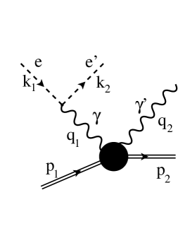
Figure 1: Kinematic of deeply virtual Compton scattering.

DVCS is the hard electro-production of a real photon, i.e. $\gamma^{*}N\to\gamma N^{\prime}$. Being a process involving a single hadron, it is one of the cleanest tools to construct generalized parton distributions (GPD) GPD ; R3 ; R4 ; R6 ; R7 , which reduce to ordinary parton distributions in the forward direction. The theoretical efforts and achievements are supported by the experimental results from HERMES, HERA and CLAS Collaborations, and encouraging future plans.

DVCS is characterized by three independent four-momenta: $p=p_{1}+p_{2},\ \Delta=p_{2}-p_{1},$ and $q=(q_{1}+q_{2})/2,$ where the vectors $p_{1}\ (q_{1})$ and $p_{2}\ (q_{2})$ refer to the incoming and outgoing proton (photon) momentum, respectively. Most of the papers on deep inelastic scattering (DIS) and DVCS are based on the operator product expansion with extensive use of the light-front variables. Otherwise, the conventional Bjorken variable is $x=\frac{Q^{2}}{2p_{1}\cdot q_{1}},\ Q^{2}=-q_{1}^{2}$, and $\xi=-\frac{q^{2}}{q\cdot P}$ is the generalized Bjorken variable. If both photons were virtual, we would have an extra scaling variable $\eta=\frac{\Delta\cdot q}{p\cdot q},$ the skewedness (or skewness) DVCS ; Pire . The reality of the outgoing photon implies the presence of only one scaling variable, namely, for $q_{2}^{2}=0$ one has

$$\eta=-\xi\Bigl{(}1+\frac{\Delta^{2}}{2Q^{2}}\Bigr{)}^{-1}.$$ (1)

The generalized and ordinary Bjorken variables are related by

$$\xi=x\frac{1+\frac{\Delta^{2}}{2Q^{2}}}{2-x+x\frac{\Delta^{2}}{Q^{2}}}.$$ (2)

Our starting point is a complex scattering amplitude depending on three variables, $\xi,t$ and $Q^{2}$, defined by Fig. 1 and the corresponding legend. Even though our paper is devoted to DIS of Fig. 2 and relevant CLAS data, we bear in mind the close relation between DVCS and DIS, the latter being the limiting case of the former.

Most of the papers on this subject are based on the factorization properties, separating the perturbative and non-perturbative dynamics (“handbag” diagram), according to which, at large $Q^{2}$, lowest order perturbation decouples from hadronic dynamics during the short time of interaction. While factorization in hard scattering processes is valid to all orders in perturbation theory, a considerable fraction of the existing data comes from so-called soft region of small and intermediate values of $Q^{2}$ ($Q^{2}\sim 1$ GeV²), where the present non-perturbative approach can be compared with the relevant successful pQCD calculations R1 ; R2 . Although $t-$ dependence at small $t$ is outside the perturbative QCD (pQCD) domain, nontrivial forms of the $t-$ dependence at a proper scale suggested recently R3 ; R4 ; R5 can be confronted to those following from Regge-dual models.

The phase of the DVCS amplitude experimentally is extracted from the interference between the DVCS and Bethe-Heitler amplitudes, like in the case of the Coulomb interference in the forward cone of elastic hadron scattering. While pQCD factorization details R1 ; R6 ; R7 how to calculate the real part of the DVCS amplitude, any Regge-dual model contains the phase explicitly, its form depending on the available freedom (form of the Regge singularity, shape of the trajectories etc) inherent in this type of models. One can hope that the results of the pQCD calculation will reduce this freedom in the future. Alternatively, this phase can be approximately reconstructed by means of the dispersion relations or their simplified version of the derivative dispersion relations, as it was done in ref. FFS .

In a series of papers we initiated the study of DIS and DVCS within a Regge-dual approach. Its virtue is the presence in the scattering amplitude of $t-$dependence and of the phase as well as its explicit energy dependence, compatible with unitarity. At high energies, the contribution of a dipole pomeron JMaP dominates, while at moderate and low energies subleading contributions (secondary reggeons) become important. Moreover, by duality, at low energies, $t-$ channel Regge pole exchanges are replaced by direct-channel reggeons.

No hard scale factorization is assumed in this approach. External photons interact with the proton via vector meson (or generalized vector meson Schild ) dominance.

The main idea behind the model is reggeization of the resonances both in the $s-$ and $t-$ channels. Nonlinear, complex Regge trajectories replace individual resonance contributions. The resulting scattering amplitude is a complex function of the Mandelstam variable $s,t,u$ and of the photon virtuality $Q^{2}$. Its imaginary part in the forward direction, $t=0$ corresponds to ordinary distributions or structure functions (SF), describing inclusive (e.g. electron-proton) scattering, while the whole amplitude is directly related to exclusive deeply virtual Compton scattering and corresponding general parton distributions.

In Refs. JMP ; JMP-1 ; FFJLM dual amplitudes with Mandelstam analyticity (DAMA) were suggested as a model for DVCS or DIS. We remind that DAMA realizes duality between direct-channel resonances and high-energy Regge behavior (“Veneziano-duality”). By introducing $Q^{2}$-dependence in DAMA, we have extended the model off mass shell and have shown JMP ; JMP-1 how parton-hadron (or “Bloom-Gilman”) duality is realized in this model. With the above specification, DAMA can serve as explicit model valid, in principle, at all values of the Mandelstam variables $s$, $t$ and $u$ as well as for any $Q^{2},$ thus realizing duality ”in two dimensions”: between hadrons and partons, on the one hand and between resonances and Regge behavior, on the other hand. The latter property opens the way of linking JLab (large x, resonances) and HERA (small x, Regge) physics.

Recently new data on inclusive electron-proton cross section in the resonance region ($W<2.5$ GeV) at momentum transfers $Q^{2}$ below $4.7$ (GeV/c)${}^{2},$ measured at the JLab (CEBAF) with the CLAS detector Osipenko were made public. In the present paper we discuss an analysis of the new CLAS data within this model.

The kinematics of inclusive electron-nucleon scattering, applicable to both high energies, typical of HERA, and low energies as at JLab, is shown in Fig. 2 (see ref. FFJLM for more details).

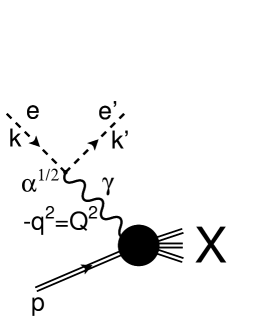
Figure 2: Kinematic of deep inelastic scattering.

Studies of the complex pattern of the nucleon structure function in the resonance region have a long history (see, for example Stein ). Among dozens of resonances in the $\gamma^{*}p$ system above the pion-nucleon threshold only a few of them can be identified more or less unambiguously. Therefore, instead of identifying each resonance, one considers a few maxima above the elastic scattering peak, corresponding to some “effective” resonance contributions. Recent results from the JLab Nicu ; Osipenko renewed the interest in the subject and they call for a more detailed phenomenological analysis of the data and a better understanding of the underlying dynamics.

The basic idea in our approach is the use the off-mass-shell continuation of the dual amplitude with nonlinear complex Regge trajectories. We adopt the two-component picture of strong interactions, according to which direct-channel resonances are dual to cross-channel Regge exchanges and the smooth background in the $s-$channel is dual to the Pomeron exchange in the $t-$channel. As explained in ref. JMP , the background in dual model corresponds to pole terms with exotic trajectories that do not produce any resonance.

II Regge-Dual Structure Function

In the present section we introduce notations, kinematics and the Regge-dual model. More details on the model can be found in earlier paper JMP ; JMP-1 ; FFJLM ; dual2 .

So, we study inclusive, inelastic electron-proton scattering, whose cross section was measured at JLab and used to determine the unpolarized structure function $F_{2}(x,Q^{2})$ as well as the Nachtmann and Cornwall-Norton moments (see e.g. Roberts ).

The cross section is related to the structure function by

$$F_{2}(x,Q^{2})={Q^{2}(1-x)\over{4\pi\alpha(1+4m^{2}x^{2}/{Q^{2}})}}\sigma_{t}^{\gamma^{*}p}~{},$$ (3)

where the total cross section, $\sigma_{t}^{\gamma^{*}p}$, includes by unitarity all possible intermediate states allowed by energy and quantum number conservation, and we follow the norm

$$\sigma_{t}^{\gamma^{*}p}(s)={\cal I}m\ A(s,Q^{2})~{}.$$ (4)

used in Refs. R8 ; JMP ; JMP-1 ; FFJLM . The center of mass energy of the $\gamma^{*}p$ system, the negative squared photon virtuality $Q^{2}$ and the Bjorken variable $x$ are related by

$$s=W^{2}=Q^{2}(1-x)/x+m^{2}~{}.$$ (5)

In the Regge-dual approach with vector meson dominance implied, Compton scattering can be viewed as an off-mass shell continuation of a hadronic reaction, dominated in the resonance region by non-strange ($N$ and $\Delta$) baryonic resonances. The scattering amplitude can be written as a pole decomposition of the dual amplitude and factorizes as a product of two vertices (form factors) times the propagator:

$$\left[A(s,Q^{2})\right]_{t=0}={\it N}\left\{\sum_{r,n}{f_{r}^{2(n-n_{r}^{min}+1)}(Q^{2})\over n-\alpha_{r}(s)}+[A(s,Q^{2})]_{t=0}^{BG}\right\}~{},$$ (6)

where $\it N$ is an overall normalization coefficient, $r$ runs over all trajectories allowed by quantum number conservation (in our case $r=N^{*}_{1},~{}N^{*}_{2},~{}\Delta$) while $n$ runs from $n_{r}^{min}$ (spin of the first resonance) to $n_{r}^{max}$ (spin of the last resonance - for more details see next section), and $[A(s,Q^{2})]_{t=0}^{BG}$ is the contribution from the background. The functions $f_{r}(Q^{2})$ and $\alpha_{r}(s)$ are respectively form factors and Regge trajectory corresponding to the $r^{th}-$term. (For a comparison of the direct-channel, ”reggeized” formula (6) with the usual Breit-Wigner expression see Appendix A). Note that only for the first resonance at each trajectory we have squared form factor, while for the recurrences the powers of form factors are growing, according to the properties of DAMA JMP ; JMP-1 .

II.1 Regge Trajectories

Any systematic account for the large number of direct-channel resonances (over 20) contributing to the $\gamma^{*}N$ total cross section with different weights is not an easy task. However, this problem can be overcome with the use of (s-channel) Regge trajectories, including all possible intermediate states in the resonance region appearing as recurrences on the trajectories. In this approach, Regge trajectories play the role of dynamical variables and the parameters of the trajectories can be fitted either to the masses and widths of the known resonances or to the data on DIS cross sections (structure functions), reflecting adequately the position of the peaks in the SF (or cross sections) formed by the interplay of different resonances.

The form of the Regge trajectories is constrained by analyticity, requiring the presence of threshold singularities, and by their asymptotic behaviour imposing an upper bound on their real part. Explicit models of Regge trajectories realizing these requirement were studied in a number of papers ReggeTraj . For our present goals (small- and intermediate energies) a particularly simple model based on a sum of square root thresholds will be suitable:

$$\alpha(s)=\alpha_{0}+\alpha_{1}s+\alpha_{2}(\sqrt{s_{0}}-\sqrt{s_{0}-s}),$$ (7)

where the lightest threshold, $s_{0}$, produces the imaginary part and the heaves thresholds producing the real part can be approximated here by a linear term. In our case JMP ; JMP-1 ; FFJLM $s_{0}=(m_{\pi}+m_{p})^{2}$.

For asymptotic, large $s-$ or $t-$ the trajectories turn down to a logarithm, producing wide angle scaling behavior with a link to the quark model. This interesting regime, discussed e.g. in ref. BJC ; JMPac , however is far away from the resonance region and will not be included in the present analyses.

In $\gamma^{*}p$ scattering, mainly the two $N^{*}$s (isospin 1/2) and one $\Delta$ (isospin 3/2) resonances contribute in the $s-$channel and thus we will limit ourselves to considering these three terms, plus an additional terms which describe the background, to be be discussed later.

II.2 Form Factors

In our previous work FFJLM , we concentrated our attention on the analytic structure of the scattering amplitudes using a simple dipole model for the form factors. However, in order to properly describe the structure function in the resonance region, it is essential to account for the helicity structure of the amplitudes. Below we do so following Davidovsky and Struminsky DS , who provided for relevant amplitudes by using the Breit-Wigner resonance model. The relation between the Breit-Wigner and the ”reggeized” resonance model, to be used can be found in Appendix A.

The form factors can be written as a sum of three terms BW ; CM86 ; CM98 ; DS , $G_{+}(Q^{2})$, $G_{0}(Q^{2})$ and $G_{-}(Q^{2})$, corresponding to $\gamma^{*}N\rightarrow R$ helicity transition amplitudes in the rest frame of the resonance $R$:

$$G_{\lambda_{\gamma}}={<R,\lambda_{R}=\lambda_{N}-\lambda_{\gamma}|J(0)|N,\lambda_{N}>\over m}~{},$$ (8)

where $\lambda_{R}$, $\lambda_{N}$ and $\lambda_{\gamma}$ are the resonance, nucleon and photon helicities, $J(0)$ is the current operator; $\lambda_{\gamma}$ takes the values $-1,0$ and $+1.$ Correspondingly, the squared form factor is given by a sum BW ; CM86 ; CM98 ; DS

$$|G_{+}(Q^{2})|^{2}+2|G_{0}(Q^{2})|^{2}+|G_{-}(Q^{2})|^{2}.$$ (9)

The explicit form of these form factors is known only near their thresholds $|\vec{q}|\rightarrow 0$, while their large-$Q^{2}$ behavior is constrained by the quark counting rules.

According to BW , one has near the threshold

$$G_{\pm}(Q^{2})\sim|\vec{q}|^{J-3/2},\ \ G_{0}(Q^{2})\sim{q_{0}\over{|\vec{q}|}}|\vec{q}|^{J-1/2}$$ (10)

for the so-called normal ($1/2^{+}\rightarrow 3/2^{-},5/2^{+},7/2^{-},...$) transitions and

$$G_{\pm}(Q^{2}\sim|\vec{q}|^{J-1/2},\ \ G_{0}(Q^{2})\sim{q_{0}\over{|\vec{q}|}}|\vec{q}|^{J+1/2}$$ (11)

for the anomalous ($1/2^{+}\rightarrow 1/2^{-},$ $3/2^{+},5/2^{-},...$) transitions, where

$$|\vec{q}|={\sqrt{(M^{2}-m^{2}-Q^{2})^{2}+4M^{2}Q^{2}}\over{2M}}\,,$$ (12)

$$q_{0}={M^{2}-m^{2}-Q^{2}\over{2M}},$$ (13)

$M$ is a resonance mass.

Following the quark counting rules, in refs. CM98 (for a recent treatment see DS ), the large-$Q^{2}$ behavior of $G$’s was assumed to be

$$G_{+}\sim Q^{-3},\ G_{0}\sim Q^{-4},\ G_{-}\sim Q^{-5}.$$ (14)

Let us note that while this is reasonable (modulo logarithmic factors) for elastic form factors, it may not be true any more for inelastic (transition) form factors. Our Regge-dual model, eq. (6), predicts that the powers of the form factors increase with increasing excitation (resonance spin). This discrepancy can be resolved only experimentally, although a model-independent analysis of the $Q^{2}$-dependence for various nuclear excitations is biased by the (unknown) background.

In ref. DS the following expressions for the $G$’s, combining the above threshold- (10), (11) with the asymptotic behavior (14), were suggested:

$$|G_{\pm}|^{2}=|G_{\pm}(0)|^{2}~{}{\it q}^{2J-3}~{}c^{2J-3}(Q^{\prime}_{0})~{}c^{m_{\pm}}(Q_{0})$$ (15)

$$|G_{0}|^{2}=C^{2}{q_{0}^{2}\over{|\vec{q}|^{2}}}{\it q}^{2J-1}c^{2a+m_{0}}(Q_{0})c^{2J-1}(Q^{\prime}_{0})$$ (16)

for the normal transitions and

$$|G_{\pm}|^{2}=|G_{\pm}(0)|^{2}{\it q}^{2J-1}~{}c^{2J-1}(Q^{\prime}_{0})~{}c^{m_{\pm}}(Q_{0})$$ (17)

$$|G_{0}|^{2}=C^{2}\left({q_{0}^{2}\over{|\vec{q}|^{2}}}\right)^{2J-1}c^{2a+m_{0}}(Q_{0})c^{2J+1}(Q^{\prime}_{0})~{},$$ (18)

for the anomalous ones, where $m_{+}=3$, $m_{0}=4$, $m_{-}=5$ count the quarks, $C$ and $a$ are free parameters. For notational convenience we have introduced the functions

$${\it q} = {|\vec{q}|\over|\vec{q}|_{Q=0}}~{},$$

$$c(z) = {z^{2}\over{Q^{2}+z^{2}}}~{}.$$

The form factors at $Q^{2}=0$ are related to the helicity photoproduction amplitudes $A_{1/2}$ and $A_{3/2}$ by

$$|G_{+,-}(0)|=\frac{1}{\sqrt{4\pi\alpha}}\sqrt{M\over{M-m}}|A_{1/2,3/2}|~{}.$$ (19)

II.3 The Background

Apart from the resonances, lying on the $N^{*}$’s and $\Delta$ $s-$channel trajectories, dual to an effective bosonic ($f$-)trajectory in the $t-$channel, one has to consider the contribution from a smooth background. Following our previous arguments, JMP ; JMP-1 ; FFJLM ; dual2 , we model it by non-resonance pole terms with exotic trajectories, dual to the Pomeron.

$$\left[A(s,Q^{2})\right]_{BG}=\sum_{b=E,E^{\prime}}G_{b}{c^{4}(Q_{b})\over n_{b}-\alpha_{b}(s)}\,.$$ (20)

with dipole form factors, given by $c^{2}(Q_{b})$. The exotic trajectories are chosen in the form

$$\alpha_{b}(s)=\alpha_{b}(0)+\alpha_{1b}(\sqrt{s_{0}}-\sqrt{s_{0}-s})~{},$$ (21)

where the coefficients $\alpha_{b}(0)$, $\alpha_{1b}$ and the $Q^{2}_{b}$ are the free parameters. To prevent any physical resonance, they are constrained in such a way that the the real part of the trajectory terminates before reaching the first resonance on the physical sheet. An infinite sequence of poles, saturating duality, appears on the non-physical sheet in the amplitude; they do not interfere in the smooth behaviour of the background (for more details see BJKSh ).

Anticipating the results of Sec. IV, we notice that fits to the data prefer a negative contribution from the second term in the background. Formally this is compatible with alternative models (e.g. Nicu ; Osipenko ), but needs to be understood also in the framework of the present Regge-dual approach.

III Comparison with other models

In this section we would like to indicate on the two important properties of our Regge-dual model, that should, in principle, discriminate it from alternative models of DIS in the resonance region.

Looking at eq. (6) one can see that contrary to the models accounting for each resonance separately here resonances on each Regge trajectory enter with progressively increasing powers of the form factors. This makes the present model quite different from the existing approaches Stein ; Nicu ; Osipenko ; DS . Notice that increasing powers of the transition form factors result in the suppression of the relevant contributions from the recurrences with growing spin, thus explaining the gradual disappearance of higher excitations. Further comparison of the experimentally measured transition form factors may discriminate between two approaches. Work in this direction is in progress.

The second important difference comes form the parameterization of the background. We describe the background by non-resonating pole terms (the poles appear on the non-physical sheet, see BJKSh ) with exotic trajectories and standard dipole form factors. The background contribution strongly decreases with increasing $Q^{2}$, whereas in ”standard” parameterizations Stein ; Nicu ; Osipenko ; DS the background is an increasing function of $Q^{2}$. Since resulting fits by different models are almost equally good, it is difficult to discriminate between these two options. Studies of the $Q^{2}-$dependence of the ratio between a resonance contributions and the background (at fix energy or x) may resolve this ambiguity and help to better disentangle resonances from the background.

IV Analysis of the CLAS data

In this section, we present our fits to the CLAS data on the nucleon structure function, $F_{2}(Q^{2},s)$ Osipenko .

A similar analysis using earlier data Nicu was carried out in our previous paper FFJLM . The main point of the model considered in FFJLM was the inclusion of three prominent resonances, $N^{*}(1520)$, $N^{*}(1680)$ and $\Delta(1232)$ plus a background, dual to the Pomeron exchange. In that approach the large number of resonances contributing to the $F_{2}$ with different wights was effectively accounted for by letting the SF to depend on effective trajectories, whose parameters were fitted to the data. This approach was, in a sense, justified “a posteriori”: the parameters of the effective trajectories were found to be close to these fitted to the spectrum of baryon resonance. Although the main features of the SF in FFJLM were reproduced by the dual model, the quality of the fit was far from perfect. The reason for the poor agreement could be threefold: first, in FFJLM we made an extra simplification by neglecting the helicity structure of the amplitudes, and the form factors were chosen in a simple dipole form. Including the spin changes the form factors in a non-trivial way and complicates the $Q^{2}-$dependence of the SF. The second point is related to the parameterization of the background: in FFJLM the background was modeled by one term only, underestimating the magnitude of the SF in some regions. The third important reason is the quality of the data - the set of points available was not homogeneous resulting in a non-uniform weight of the fit. To cure this deficiency, we performed a preselection of the initial data set, a procedure that potentially may results in ambiguities. The fits were improved, although still are not perfect.

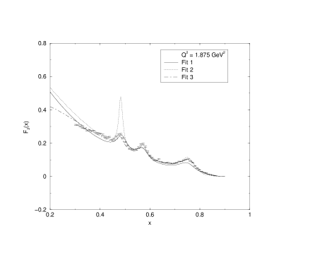
Figure 3: Comparison between three different fits performed in the present model (see text).

Similarly to FFJLM , here we also include only the contribution from three dominant resonances: $N^{*}(1520)$, $N^{*}(1680)$ and $\Delta(1232)$ and we implement this by using three baryon trajectories with one resonance on each of them. By considering such resonances as “effective” contributions to the SF, we are able to treat the large number of resonances that contribute, with different weights, to the SF.

The imaginary part of the scattering amplitude can then be written, according to (6), as a sum of the contribution from the resonances plus the background,

$${\cal I}m\ A(s,Q^{2})={\it N}\left\{[{\cal I}m\ A(s,Q^{2})]_{R}+[{\cal I}m\ A(s,Q^{2})]_{BG}\right\}~{}.$$

Accordingly, the resonance contribution takes the following form:

$$[{\cal I}m\ A(s,Q^{2})]_{R}=\sum_{j=\Delta,~{}N_{1},~{}N_{2}}f^{2}_{j}(Q^{2}){{\cal I}m_{j}\over(n_{j}-{\cal R}e_{j})^{2}+{\cal I}m_{j}^{2}}~{},$$

with ${\cal R}e\$ and ${\cal I}m\$ denoting the real and imaginary part of the relevant Regge trajectory, and the form factors are calculated as described in sec. II.2. For instance, the form factor for the $\Delta$ resonance can be written as

$$f_{\Delta}^{2}(Q^{2})={\it q}^{2}c^{2}(Q^{\prime}_{0})\left(c^{3}(Q_{0})|G_{+}(0)|^{2}+c^{5}(Q_{0})|G_{-}(0)|^{2}\right)\;;$$ (22)

similar expressions can be cast for other contributions.

The imaginary part of the forward scattering amplitude coming from the background can be easily obtained from (20):

$$[{\cal I}m\ A(s,Q^{2})]_{BG}=\sum_{j=E,E^{\prime}}G_{j}~{}c^{4}(Q_{j})~{}{{\cal I}m_{j}\over(n_{j}^{min}-{\cal R}e_{j})^{2}+{\cal I}m_{j}^{2}}~{}.$$

Here $n_{j}^{min}$ is the lowest integer, larger than Max $[{\cal R}e_{j}]$, ensuring that no resonances will appear on the exotic trajectory. The advantage of such choice is that the two terms of the background depend on two different scales, $Q^{2}_{E}$ and $Q^{2}_{E^{\prime}}$, so they will dominate in different regions.

The model constructed in this way, has 23 free parameters: each resonance is characterized by three (the intercept is kept fixed) coefficients describing the relevant Regge trajectory plus the two helicity photoproduction amplitudes (see eq. (19)). The form factors (see sec. II.2) leave only two free parameters, $Q_{0}$ and $Q^{\prime}_{0}$. Finally, the background, contains 8 free parameters: 4 for the two exotic trajectories, 2 energy scales $Q_{E}$ and $Q_{E^{\prime}}$ and two amplitudes $G_{E}$ and $G_{E^{\prime}}$. With the overall normalization factor, $\it N$ this gives a total of 23 free parameters.

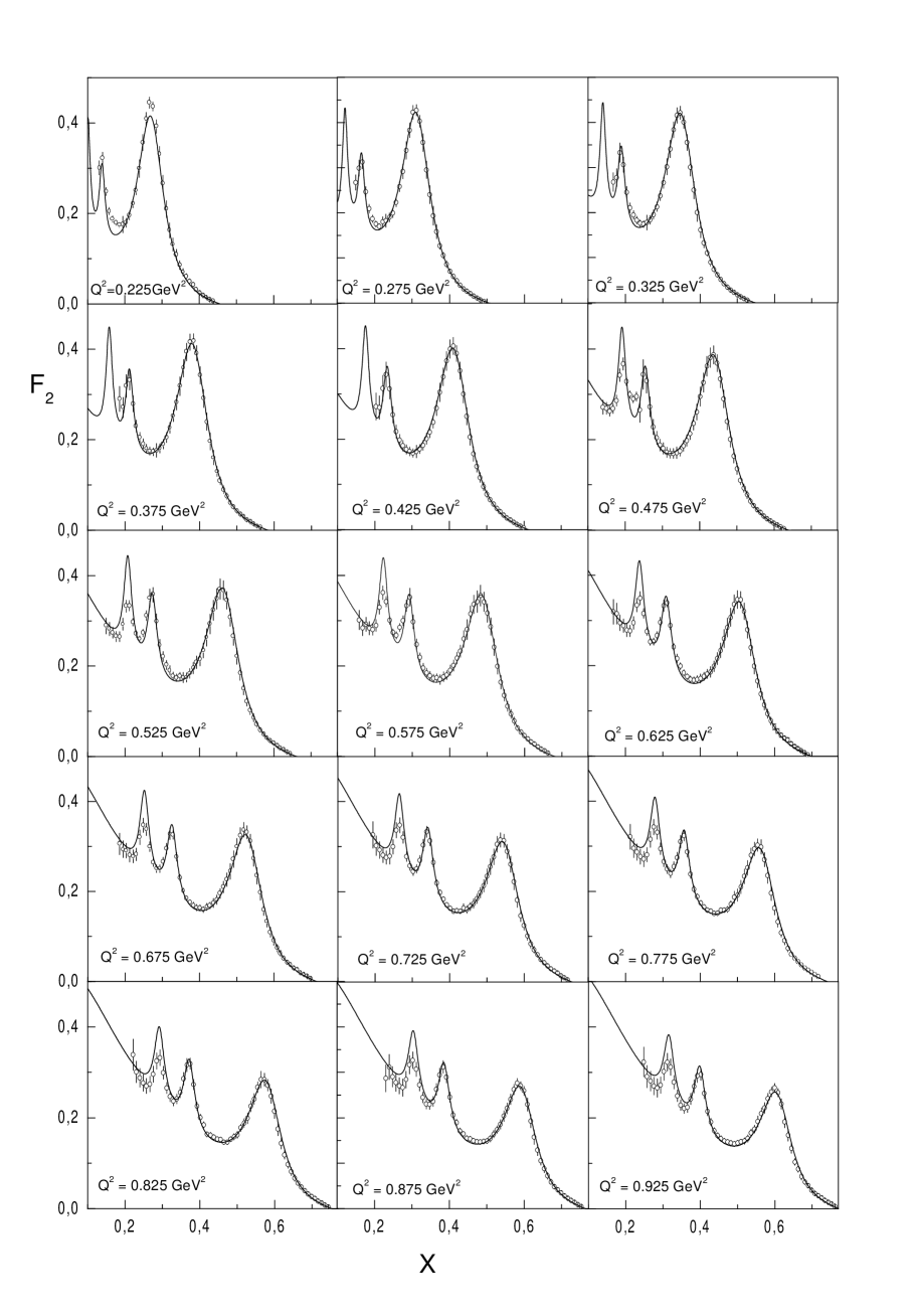
Figure 7: Structure function $F_{2}(x)$ for $Q^{2}=0.225-0.925$ GeV². Data are from Osipenko , whereas the straight line is the prediction of our dual model.

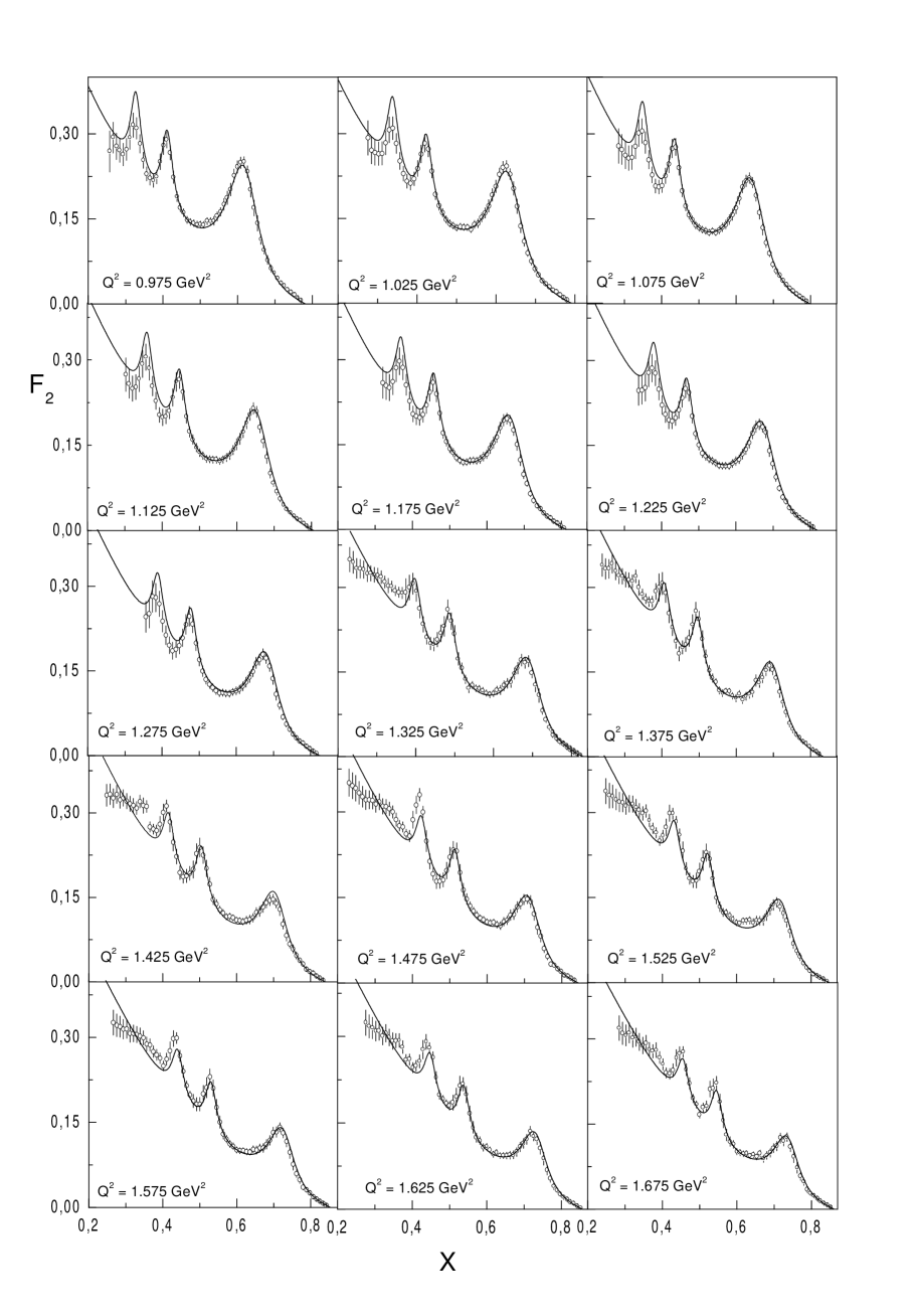
Figure 8: Structure function $F_{2}(x)$ for $Q^{2}=0.975-1.675$ GeV².

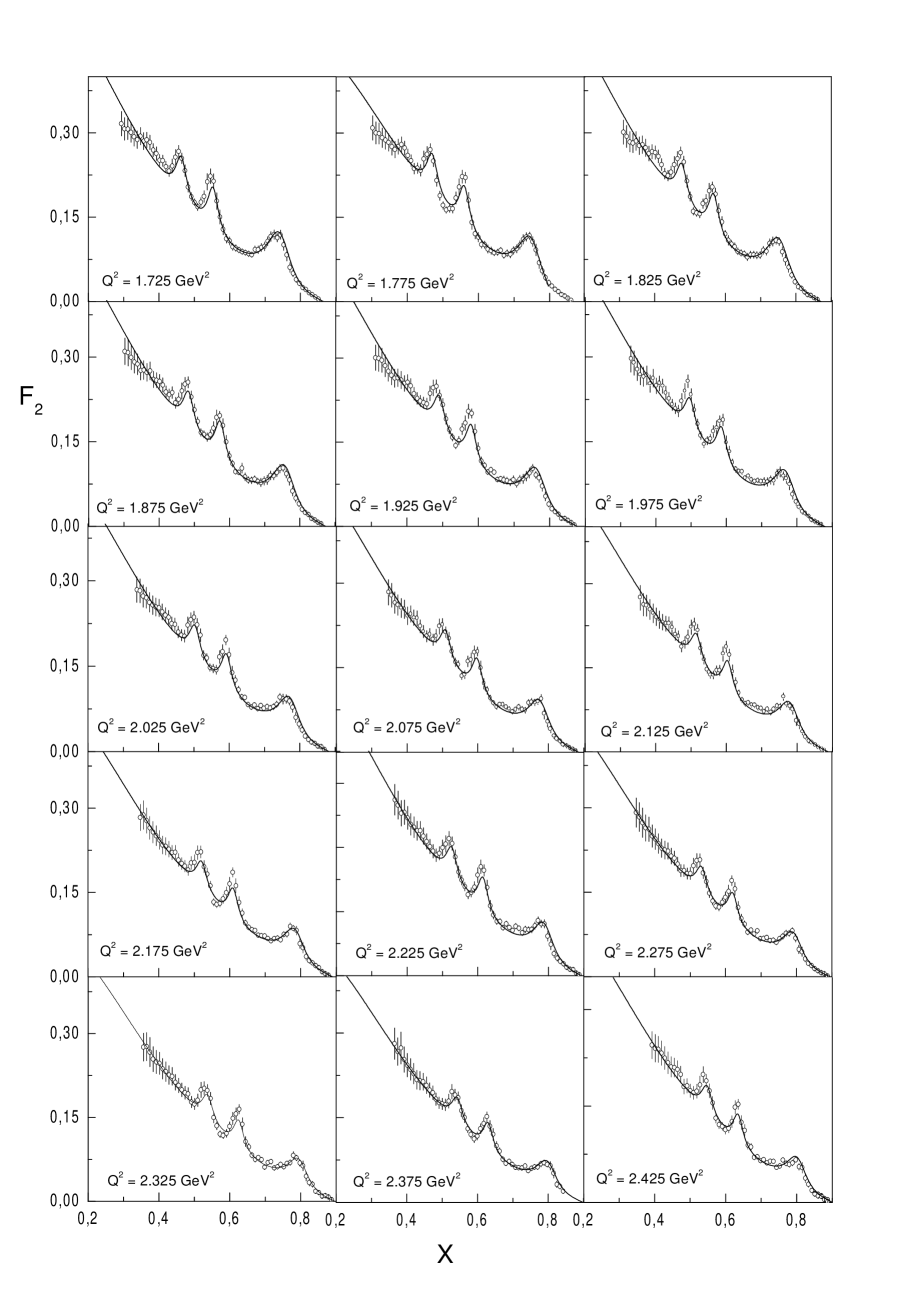
Figure 9: Structure function $F_{2}(x)$ for $Q^{2}=1.725-2.425$ GeV².

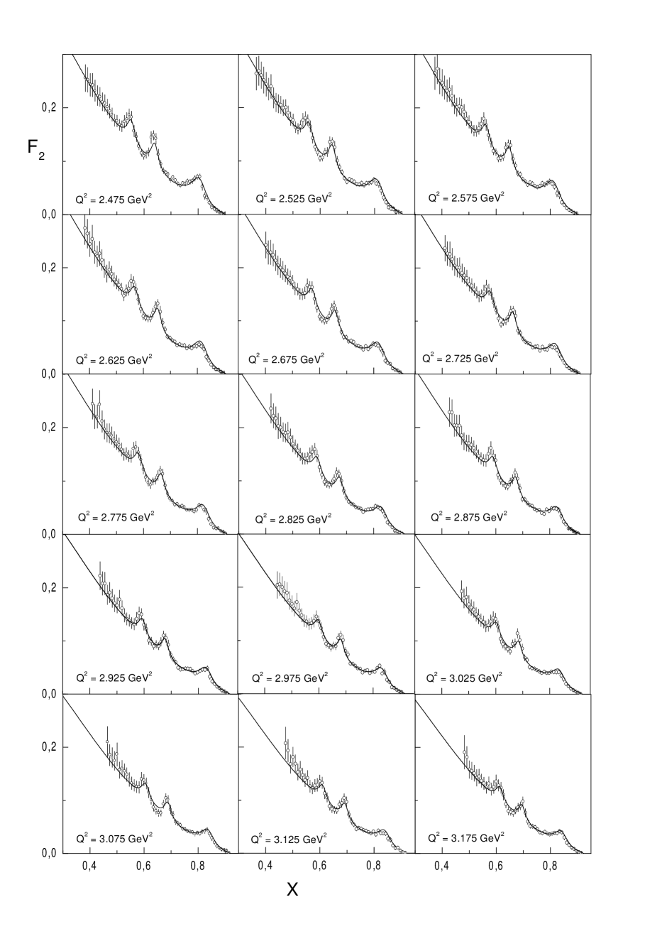
Figure 10: Structure function $F_{2}(x)$ for $Q^{2}=2.475-3.175$ GeV².

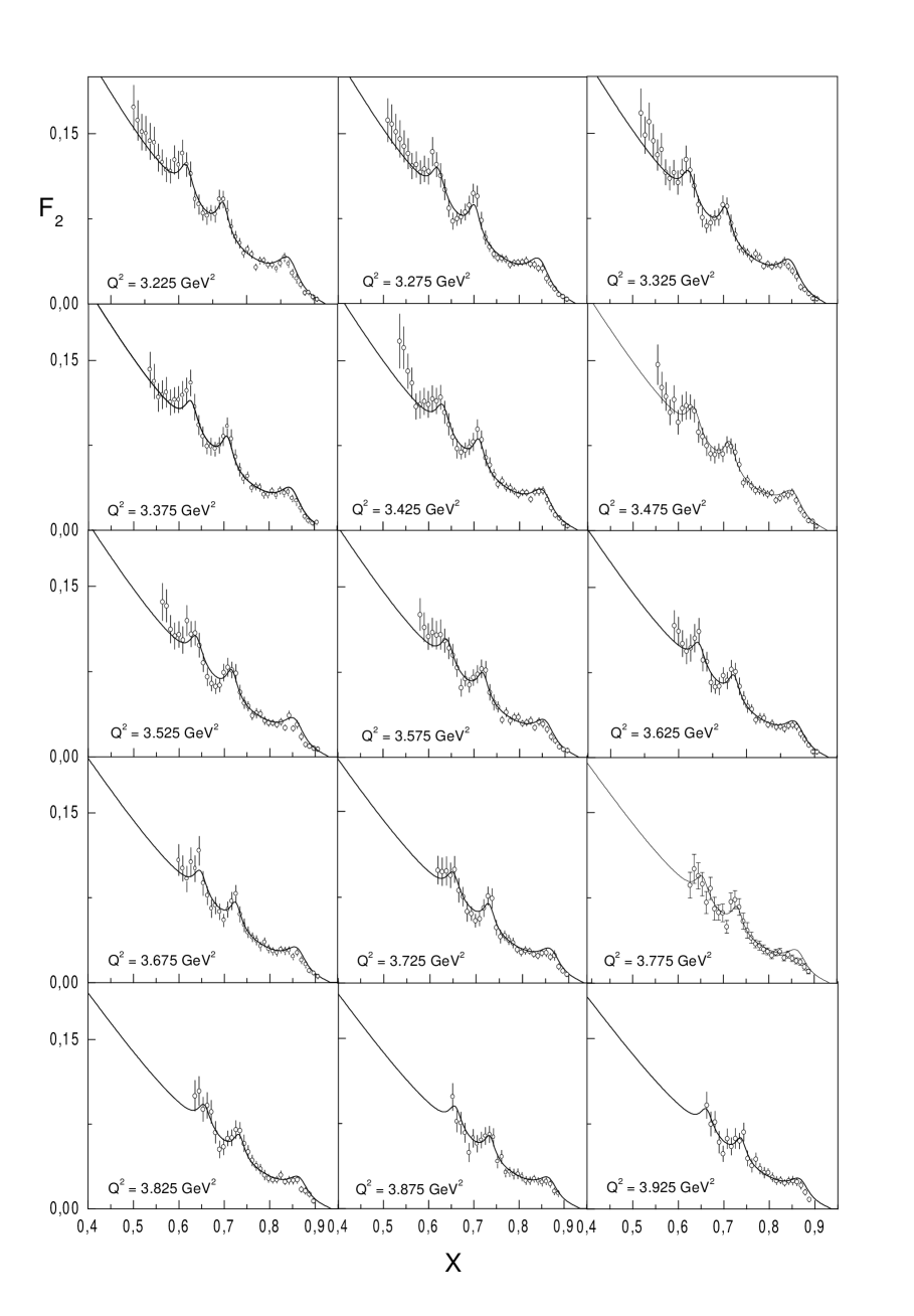
Figure 11: Structure function $F_{2}(x)$ for $Q^{2}=3.225-3.925$ GeV².

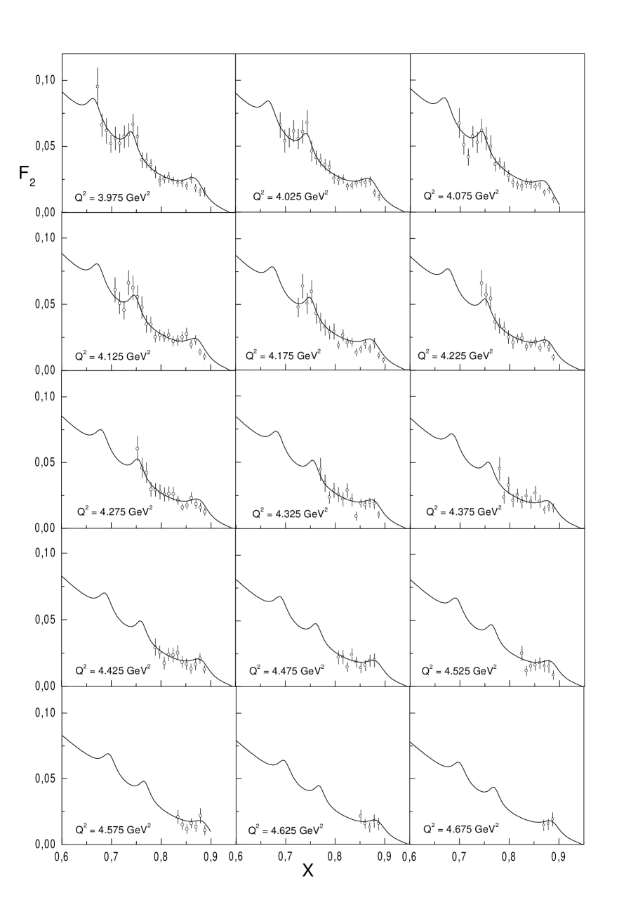
Figure 12: Structure function $F_{2}(x)$ for $Q^{2}=3.975-4.675$ GeV².

The resulting fits to the CLAS data, performed by using MINUIT minuit , are presented in Table 1 and together with the experimental data is shown for various $Q^{2}$ bins in Figs. (7-12).

	parameters	Fit 1	Fit 2	Fit 3
	$\alpha_{0}$	-0.8377⋄	-0.8377⋄	-0.8377⋄
	$\alpha_{1}$ [GeV-2]	0.9500⋄	0.9402	0.9825
$N_{1}^{*}$	$\alpha_{2}$ [GeV-1]	0.1473⋄	0.1757	0.0920
	$A^{2}(1/2)$ [GeV-1]	0.0484E-2⋄	0.0484E-2⋄	0.8647E-2
	$A^{2}(3/2)$ [GeV-1]	0.2789E-1⋄	0.2789E-1⋄	0.9634E-2
	$\alpha_{0}$	-0.3700⋄	-0.3700⋄	-0.3700⋄
	$\alpha_{1}$ [GeV-2]	0.9500⋄	0.9724	0.9551
$N_{2}^{*}$	$\alpha_{2}$ [GeV-1]	0.1471⋄	0.0575	0.0949
	$A^{2}(1/2)$ [GeV-1]	0.0289E-2⋄	0.0289E-2⋄	0.9724E-2
	$A^{2}(3/2)$ [GeV-1]	0.1613⋄	0.1613⋄	5.1973E-11
	$\alpha_{0}$	0.0038⋄	0.0038⋄	0.0038⋄
	$\alpha_{1}$ [GeV-2]	0.8500⋄	0.8758	0.8605
$\Delta$	$\alpha_{2}$ [GeV-1]	0.1969⋄	0.1724	0.2005
	$A^{2}(1/2)$ [GeV-1]	0.0199⋄	0.0199⋄	5.3432E-08
	$A^{2}(3/2)$ [GeV-1]	0.0666⋄	0.0666⋄	0.0866
	G${}_{E_{1}}$	6.5488	2.8473	3.6049
	$\alpha_{0}$	0.3635	0.7014	0.3883
	$\alpha_{2}$ [GeV-1]	0.1755	0.1575	0.3246
$E_{1}$	$Q_{E_{1}}^{2}$ [GeV2]	5.2645	4.5169	3.9774
	$s_{E_{1}}$ [GeV2]	1.14⋄	1.3038	1.14⋄
	G${}_{E_{2}}$	—	—	-0.6520
	$\alpha_{0}$	—	—	-0.8929
$E_{2}$	$\alpha_{2}$ [GeV-1]	—	—	1.7729
	$Q_{E_{2}}^{2}$ [GeV2]	—	—	2.4634
	$s_{E_{2}}$ [GeV2]	—	—	1.14⋄
	$s_{0}$ [GeV2]	1.14⋄	1.14⋄	1.14⋄
	$Q^{{}^{\prime}2}_{0}$ [GeV2]	0.4089	0.4580	0.9998
	$Q_{0}^{2}$ [GeV2]	3.1709	2.5180	1.8926
	${\it N}$ [GeV-2]	0.0408	0.0655	0.0567
	$\chi^{2}_{d.o.f.}$	12.92	4.6886	1.3005

Table 1. Parameters of the fits. The symbol ^⋄ refers to the fixed parameters.

To start with, we made a fit by keeping some of the parameters fixed, close to their physical values, particularly those of the Regge trajectories and of the photoproduction amplitudes. Also, a single-term background was used. The resulting fit (fit 1) is shown in Table 1. Next (fit 2) some of the parameters of the Regge trajectory were varied. Consequently the $\chi^{2}$ was improved, although still remaining unsatisfactory. Finally, we let all the parameters vary (fit 3) with the result reported in the Table. Fit 3 is good, with $\chi_{d.o.f.}=1.30$. It is worth mentioning that a comparison with a similar fit performed in dual2 leading to $\chi_{d.o.f.}=9.4$ needs care, since in dual2 only one term in the background was included, the helicity amplitudes were kept constant and the dataset used included both data from Nicu and Osipenko .

To show the progress in the fits, we plot against the experimental data the structure functions for four different values of $Q^{2}$ with the parameters from three different fits - see Fig. 3 .

Having fitted the parameters (from now on we will use parameters of fit 3), we can now proceed to further calculations (moments) and analyses (duality relations) of the model.

V Moments

We have calculated the moments of the structure functions using the explicit expressions and parameters fitted in the previous section. These moments can be used, in particular, to estimate the role of the non-perturbative effects (higher twists).

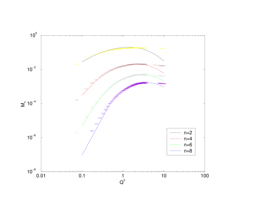
Figure 4: Nachtmann moments, $M_{n}^{N}$ for $n~{}=~{}2,~{}4,~{}6,~{}8$. The plot compares the moments calculated from the Regge-dual with those extracted from the data and reported in Osipenko (inelastic part).

From the operator product expansion (for a comprehensive review see e.g. Roberts ) the moments $M_{n}(Q^{2})$ of $F_{2}$ are defined as

$$M_{n}(Q^{2})=\sum_{J=2k}^{\infty}E_{nJ}(\mu,Q^{2})O_{nJ}(\mu)\left({\mu^{2}\over Q^{2}}\right)^{(J-2)/2}~{},$$ (23)

where $k=1,2,...$, $\mu$ is a factorization scale, $O_{nJ}(\mu)$ is the reduced matrix element of the local operators with definite spin $n$ and twist $J$, related to the non-perturbative structure of the target, $E_{nJ}(\mu,Q^{2})$ is a dimensionless coefficients related to the small distance behaviour.

The leading twist term $\tau=2$ is well established in pQCD, while higher twists are indicators of the non-perturbative and confining effects. In order to study the higher twists, it is essential to have a complete knowledge of the $F_{2}$ covering the entire $x-$range for each fixed $Q^{2}$. Higher twists can be well established only with higher moments ($n~{}>~{}2$), meanwhile for $M_{2}$ their contribution is small even at $Q^{2}\sim 1$ GeV². Therefore the most interesting kinematical region lies between $0$ and $5$ GeV² and large values of $x$, where the higher moments dominate. The JLab data and relevant calculations in Osipenko cover most of this region.

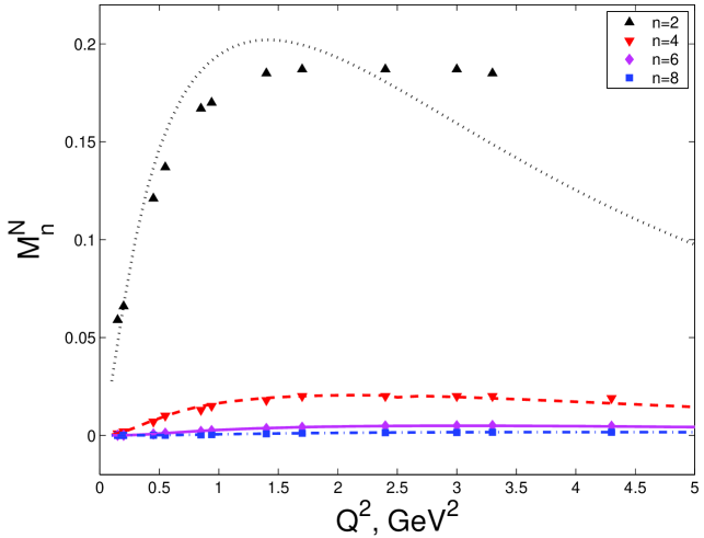
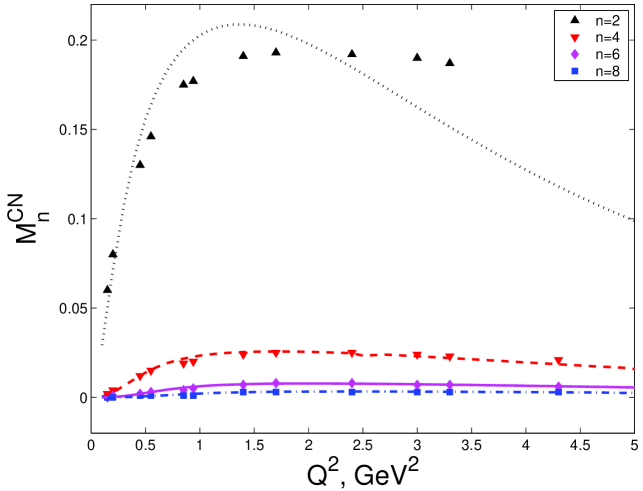
Figure 5: Nachtmann moments, $M_{n}^{N}$, and Cornwall-Norton moments, $M_{n}^{CN}$, for $n~{}=~{}2,~{}4,~{}6,~{}8$. These plots show the comparison between the moments evaluated according to our Regge-dual model and the values of the moments extracted from the electron-proton scattering data reported in armstrong (inelastic part).

In the present section we evaluate the Nachtmann (N) and Cornwall-Norton (CN) moments within our Regge-dual model and compare them with the data of the CLAS colaboration Osipenko as well as with those from ref. armstrong .

The relevant moments are defined as

$$M_{n}^{I}(Q^{2})=\int_{0}^{1}dxp_{n}^{I}(x)F_{2}(x,Q^{2})$$ (24)

where

$$p^{I}_{n}(x)=\left\{\begin{minipage}[c]{142.26378pt} ${\xi^{n+1}\over x^{3}}{\it P}(x,Q^{2})$ for I= N \\ $x^{n-2}$,~{}~{}~{}~{}~{}~{}~{}~{}~{}~{}for I = CN \end{minipage}\right.$$

$${\it P}(x,Q^{2}) = \left[{3+3(n+1)r+n(n+2)r^{2}\over(n+2)(n+3)}\right]~{},$$

$$r = \sqrt{1+4M^{2}x^{2}/Q^{2}}~{},$$

$$\xi = 2x/(1+r)~{}.$$

Please note that in our calculations the elastic part of the SF (for $x=1$) was not taken into account (see section III.G in Ref. Osipenko ).

It is a relatively simple task to obtain the moments by using the existing numerical integration methods. We have used the parameters of fit 3 from Table 1. In Fig. 4 we plot the Nachtmann moments for $n=2,~{}4,~{}6,~{}8$ together with the results from Osipenko . In Fig. 5, the calculated N- and CN-moments are compared with those from armstrong . On this second set of figures the errors in the momenta are not displayed; according to armstrong they should be less than 5$\%$.

As seen from the figures, the agreement between our model and the data is quite good in the region $Q^{2}<5$ GeV², where the SFs were fitted to the data. The discrepancies increase with $Q^{2}$, away from the measurements.

VI Duality Ratio

In this section we check the validity of the parton-hadron duality for our Regge-dual model by calculating the so-called ‘duality ratio’

$$I(Q^{2})={I_{Res}\over I_{Scaling}}$$ (25)

where

$$I_{scaling}(Q^{2}) = \int_{s_{min}}^{s_{max}}ds\ F_{2}^{scaling}~{},$$

$$I_{Res}(Q^{2}) = \int_{s_{min}}^{s_{max}}ds\ F_{2}^{Res}~{},$$

and we have fixed the lower integration limit $s_{min}=s_{0},$ varying the upper limit $s_{max}$ equal $5$ GeV ² and $10$ GeV². These limits imply ”global duality”, i.e. a relation averaged over some interval in $s$ (contrary to the so-called ”local duality”, assumed to hold at each resonance position). For fixed $Q^{2}$ the integration variable can be either $s$ (as in our case), $x$ or any of its modifications ($x^{\prime},\ \xi,...$) with properly scaled integration limits. The difference may be noticeable at small values of $Q^{2}$ due to the target mass corrections (for details see e.g. Osipenko ). These effects are typically non-perturbative and, apart from the choice of the variables, depend on detail of the model.

In choosing the smooth ”scaling curve” $F_{2}^{scaling}$ (actually, it contains scaling violation, in accord with the DGLAP evolution) we rely on a model developed in csernai and based on a soft non-perturbative Regge pole input with subsequent evolution in $Q^{2}$, calculated csernai from the DGLAP equation.

The function $F_{2}^{Res}$ is our SF with the parameters of fit 3 (see Table 1). The results of the calculations for different values of $s_{max}$ are shown in Fig. 6.

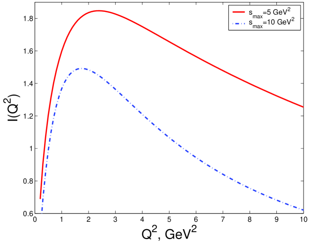
Figure 6: Global parton-hadron duality test for different values of $s_{max}$

Given the available variety and flexibility of the existing parameterizations for the SFs (see Sec. III) we do no attribute too much importance to the above duality test. Its validity or failure to large extent may be caused by accidental interplay of the details of different parameterizations. By this we do not intend to raise doubts about the very concept of parton-hadron duality. Moreover, in our opinion, explicit realization of this concept, similar to the Veneziano model, should exist and looked for. Work in this direction is in progress.

VII Conclusions

The main objective of the present study is a phenomenological analyses of the CLAS data in a model within the analytical $S$ matrix approach, complementary to approaches based on pQCD. This analyses, as well as similar attempts show that achieving good fits (with low $\chi^{2}$) to the data is a highly nontrivial task by itself. The origin of this difficulty is the large number and high statistics of the data and poor understanding of the non-perturbative dynamics, typical of the kinematical region where data are collected.

As repeatedly stressed, our approach does not compete with QCD; it is aimed to be complementary to QCD in the non-perturbative domain. The main virtue of our Regge-dual approach is its generality: potentially, it can be used for any value of its kinematical variable. From this point of view, of special interest is the possibility to link low-energy, resonance physics (and the JLab data) with the high-energy (or low x) physics (from HERA) by ”Veneziano duality” (apart from parton-hadron duality), inherent in the model.

The price for such generality is the available freedom or flexibility of the model. It can be, however, further limited by comparison with other models, pQCD calculations and the data. In particular,

1. Realistic parameterizations for baryonic trajectories, satisfying the theoretical constraints yet fitting the data, should be further elaborated. Work in this direction is in progress.

2. The separation of resonances from background is model-dependent. Our parameterization of the background differs from that introduced long ago (see e.g. Stein ) and used in all subsequent papers (e.g. Nicu ; Osipenko . Its non-orthodox motivation comes from dual analytical models. At the same time, fits to the data produce (see Sec. IV) a negative sign in front of the second term of the background, similar to the ”orthodox” models (e.g. Nicu ; Osipenko ).

3. The present Regge-dual approach generalizes the concept of transition form factors, continuous in spin. Moreover, higher spin resonance excitations are accompanied by higher powers of the relevant transition form factor, and since the Regge trajectories imply an analytic continuation in spin, the same applies for the transition form factors.

On the whole, the revival of the analytical methods, namely the study of various Riemann sheets of the scattering amplitude in the resonance region (for a recent interesting approach along these lines see osip ), and its combinations with the parton model and QCD is a promising new development in the strong interaction theory, that may shed new light on the confinement problem.

In estimating the predictive power (or flexibility) of the present model, we notice that the number of the free parameters here (23) is comparable or smaller to that in similar fits. For example I. Niculescu dissNicu uses 30 fitting parameters. The virtue of the present Regge-dual approach is the possibility to extend the model using the same set of the parameters to the small x domain, treated in Refs. FJM ; JMP ; JMP-1 . Matching the large-x (Jlab) and small-x (HERA) kinematical regions will remove or at least reduce substantially the number of the free parameters and the constrain the flexibility of the model. The realization of this ambitious goal, already discussed in Refs. FJM ; JMP ; JMP-1 , will depend on the right choice of the $Q^{2}$ dependence or, alternatively, the correct off mass shell continuation of the dual amplitude. In the present paper $Q^{2}-$ dependence was introduced in the resonance region via the transition form factors.

To conclude, let us once more emphasize that the Regge-dual approach to DIS and DVCS to large extent is complemental to the conventional one, based on the presence of a hard scale, when $Q$ (or a mass $M$) is large and the amplitude is calculable up to corrections of $1/Q$ times logarithms of $Q^{2}$. In this case hard-scattering factorization can be applied for any $x$, small or not.

In the standard approach the generalization of DIS structure functions to the DVCS amplitude can be illustrated Diehl by the following sequence of transitions

$$F_{2}\sim{\cal I}m\ A(\gamma^{*}p\rightarrow\gamma^{*}p)\rightarrow{\cal I}m\ A(\gamma^{*}p\rightarrow\gamma p)_{t=0}\rightarrow A(\gamma^{*}p\rightarrow\gamma p)_{t=0}\rightarrow A(\gamma^{*}p\rightarrow\gamma p)\,.$$ (26)

In phenomenological approaches, $t-$ dependence usually is introduced by simply multiplying the forward scattering amplitude by arbitrary exponential $e^{Bt}$, incompatible with the shrinkage of the cone. A consistent, non-factorizable form of the $t-$ dependence was discussed and derived within pQCD in a recent interesting paper by Freund R5 .

In the Regge-dual approach, on the other hand, the above sequence can be inverted: on starts with a complex, $t-$ dependent DVCS amplitude that can be reduced to the DIS structure function $F_{2}$ by taking its imaginary part, setting $t=0$ and equating the two photon momenta. This approach does not require the presence of any hard scale, such as large photon momenta. The external photons are assumed to couple to the proton by vector dominance (or generalized vector dominance Schild ). In this sense this approach is typically ”non-perturbative”. Partons (quarks and gluons) are not present explicitly but rather implicitly, manifest in the scaling behavior of the amplitude for large $s,t$ and/or $Q^{2}$, as well as in the values of the parameters (e.g. quark counting). The link between the scaling behavior of the analytic and quark models is a very interesting but still open problem. It was approached in a number of papers, e.g. in JMPac , where the large angle scaling behavior in a dual model was achieved by using Regge trajectories with logarithmic asymptotic behavior.

Although ours is a typically ”soft” approach, the quark structure, small-distance effects, etc are also present their due to the use of nonlinear Regge trajectories. In particular, the asymptotic logarithmic behavior of these trajectories could mimic hard scattering, quark counting etc. SchSch ; JMPac . These effects are not factorized, as in the standard approach of DVCS and in most of the related papers, but are continuous, i.e. the transition from ”hard” (perturbative) to ”soft” (non-perturbative) dynamics occurs smoothly, according to the properties of dual analytical models. The correspondence between the ”hard” sector of this dual model and pQCD (or the quark model) (see e.g.SchSch ; BJC ) is an interesting problem, meriting further studies.

VIII Acknowledgments

We thank M. Osipenko for a useful correspondence. L.J. and V. M. acknowledge the support by INTAS under Grant 00-00366. The work of A.F. is supported by the European Community via the award of a ‘Marie Curie’ postdoctoral Fellowship. A.F. acknowledges the support of FEDER under project FPA 2002-00748. This work has been partially supported by the Ministero dell’Istruzione dell’Universita’ e della Ricerca.

Appendix A Pole decomposition of the dual amplitude and the Breit-Wigner formula

In the vicinity of a resonance, the nucleon structure function can be can be written in a factorized form CM98 :

$$F_{2}(x,Q^{2})=\frac{m\nu Q^{2}}{\nu^{2}+Q^{2}}\delta(W^{2}-M^{2})\,\times P_{F}(Q^{2})\,$$ (27)

where $P_{F}(Q^{2})$ stands for some power of the nucleon (transition) form factor: this power is two in the standard approach, as e.g. in ref. Stein ; Nicu ; Osipenko ; DS , but varies (rises) with the resonances spin in the present Regge-dual approach; $\nu={p\,\cdot q\over m}=\frac{Q^{2}}{2mx}$ ($p$ is the four-dimensional momentum of the nucleon, $q$ is the four-dimensional momentum of photon, see Fig. 2), and $M$ is the mass of the resonance.

This formula determines the contribution of a single, infinitely narrow resonance to nucleon structure functions. For a wide resonance, if we replace the delta-function $\delta(W^{2}-M^{2})$ in the above expression by the familiar Breit-Wigner formula

$$\frac{1}{\pi}\,\frac{M\Gamma}{(W^{2}-M^{2})^{2}+M^{2}\Gamma^{2}}\,,$$ (28)

where $\Gamma$ is the resonance width, what leads to the following expression DS :

$$F_{2}(x,Q^{2})=\frac{2m^{2}x}{1+4m^{2}x^{2}/Q^{2}}\;\frac{1}{\pi}\frac{M\Gamma}{(m^{2}+Q^{2}(1/x-1)-M^{2})^{2}+M^{2}\Gamma^{2}}\times P_{F}(Q^{2})\,.$$ (29)

Now let us compare this expression with our eq. (22):

$$F_{2}(x,Q^{2})={Q^{2}(1-x)\over{4\pi\alpha(1+4m^{2}x^{2}/{Q^{2}})}}{\it N}{{\cal I}m_{j}\over{(n_{j}-{\cal R}e_{j})^{2}+{\cal I}m_{j}^{2}}}\times P_{F}(Q^{2})~{},$$ (30)

Expanding the Regge trajectory near a resonance: ${\cal R}e_{j}\approx n_{j}+\{{\cal R}e\ \alpha_{j}\}^{{}^{\prime}}(s-M^{2})=n_{j}+\{{\cal R}e\ \alpha_{j}\}^{{}^{\prime}}(m^{2}+Q^{2}(1/x-1)-M^{2})$ and introducing the notation: $\Gamma=\frac{{\cal I}m_{j}}{\{{\cal R}e\ \alpha_{j}\}^{{}^{\prime}}M}$, we get the expression:

$$F_{2}(x,Q^{2})={Q^{2}(1-x)\over{4\pi\alpha(1+4m^{2}x^{2}/{Q^{2}})}}\frac{\it N}{\{{\cal R}e\ \alpha_{j}\}^{{}^{\prime}}}\frac{M\Gamma}{(m^{2}+Q^{2}(1/x-1)-M^{2})^{2}+M^{2}\Gamma^{2}}\times P_{F}(Q^{2})~{}.$$ (31)

Notice that $Q^{2}(1-x)=(s-m^{2})x\approx(M^{2}-m^{2})x$ in the vicinity of the resonance and therefore eqs. (29) and (31) are approximately the same for

$${\it N}=\frac{8m^{2}\alpha\{{\cal R}e\ \alpha_{j}\}^{{}^{\prime}}}{(M^{2}-m^{2})}\,.$$ (32)

The obtained value for the normalization coefficient is approximately (for $M=\sqrt{2}\ m$ and $\{{\cal R}e\ \alpha_{j}\}^{{}^{\prime}}=1$ GeV^-2) ${\it N}\approx 8\alpha=0.058$ GeV^-2, in agreement with the results of the fit (see Table 1).

References

- (1) J. Blümlein, B. Geyer and D. Robaschik, Nucl. Phys. B560 (1999) 283; P.A.M. Guichon and M. Vanderhaeghen, Prog. Part. Nucl. Phys. 41 (1998) 125;
- (2) A.V. Belitsky, D. Müller, A, Kirschner, Nucl. Phys. B629 (2002) 323.
- (3) A. Freund, M. McDermott, M. Strikman, Phys.Rev. D67 (2003) 036001.
- (4) A. Freund, hep-ph/0306012.
- (5) D. Müller et al., Fotschr. Phys. 42 (1994) 101; M. Diehl et al., Phys. Lett. B411 (1997) 193; X. Ji, Phys. Rev. Lett. 78 (1997) 610; M. Diehl, hep-ph/0307382.
- (6) K. Goeke, M.V. Polyakov, M. Vanderhaeghen, Prog. Part. Nucl. Phys. 47 (2001) 401.
- (7) A. Mukherjee, I.V. Musatov, H.C. Pauli, A.V. Radyushkin, Phys.Rev. D67 (2003) 073014.
- (8) A.V. Radyushkin, Phys. Rev. D56 (1997) 5524.
- (9) A. Freund, M.F. McDermott Phys. Rev. D65 (2002) 056012, Erratum-ibid. D66 (2002) 079903.
- (10) J.P. Ralston, B. Pire, Phys. Rev. D66 (2002) 111501; B. Pire, hep-ph/0211093.
- (11) L.L. Frankfurt, A. Freund, M. Strickman, Phys. Lett. B460 (1999) 417; L.L. Frankfurt, A. Freund and M. Strickman, Phys. Rev. D58 (1998) 114001; D59 (1999) 119901.
- (12) L.L. Jenkovszky, E.S. Martynov, F. Paccanoni, hep-ph/9608384; R. Fiore, L.L. Jenkovszky, F. Paccanoni, Eur. Phys. J. C10 (1999) 461; E. Martynov, E. Predazzi , A. Prokudin, Eur. Phys. J. C26 (2002) 271; hep-ph/0211430.
- (13) M. Kuroda, D. Schildknecht Phys.Rev. D66 (2002) 094005.
- (14) L.L. Jenkovszky, V.K. Magas, E. Predazzi, Eur. Phys. J. A12 (2001) 361.
-
(15)
L.L. Jenkovszky, V.K. Magas, E. Predazzi, nucl-th/0110085;
L.L. Jenkovszky, V.K. Magas, hep-ph/0111398; R. Fiore et al., hep-ph/0212030. - (16) R. Fiore et al., Eur. Phys. J. A15 (2002) 505.
- (17) M. Osipenko et al., Phys. Rev. D 67 092001 (2003); hep-ex/0309052.
- (18) S. Stein et al., Phys. Rev. 12 (1975) 1884.
- (19) I. Niculescu et al., Phys. Rev. Lett. 85 (2000) 1182; ibid. 1186.
- (20) A. Flachi et al. Ukrainian Physics Journal 48 (2003) 507.
- (21) R.G. Roberts, The Structure of the Proton, Cambridge University Press, 1990.
- (22) P. Desgrolard, A. Lengyel, E. Martynov Eur. Phys. J. C7 (1999) 655.
- (23) G. Cohen-Tannoudji, V.V. Ilyin, L.L. Jenkovszky, R.S. Tutik, Lett. Nuovo Cim. 5 (1972) 957; A.I. Bugrij, N.A. Kobylinsky, Annalen der Phys. 32 (1975) 297; A.A. Trushevsky, Ukr. Fiz. Zh. 22 (1977) 353; L.L. Jenkovszkly, Fortschr. Phys. 34 (1986) 791; R. Fiore et al, Eur. Phys. J. A10 (2001) 217; Nucl. Phys. Proc. Suppl. 99A (2001) 68.
- (24) A.I. Bugrii et al., Z. Phys. C4 (1980) 45.
- (25) L.L. Jenkovszky, V.K. Magas and F. Paccanoni, Phys. Rev. D 60 (1999) 116003.
- (26) V.V. Davydovsky and B.V. Struminsky, Ukrainian Journal of Physics 47 (2002) 1123, hep-ph/0205130.
- (27) J.D. Bjorken, J.D. Walecka, Ann. Physics 38 (1966) 35.
- (28) C.E. Carlson, Phys. Rev. D34 (1986) 2704.
- (29) C.E. Carlson, N.C. Mukhopadhyay, Phys. Rev. D58 (1998) 094029.
- (30) A.I. Bugrij, L.L. Jenkovszky, N.A. Kobylinsky, Lett. Nuovo Cim. 5 (1972) 389.
- (31) MINUIT - function minimization and error analysis, CERN program library entry D506, CERN.
- (32) C.S. Armstrong et al., Phys. Rev. D63 (2001) 094008.
- (33) L. Csernai et al., Eur. Phys. J. C24 (2002) 205.
- (34) M. Osipenko, hep-ph/0307316.
- (35) I. Niculescu, Inclusive resonance eletroproduction data from hydrogen and deutherium and studies of quark-hadron duality, Thesis, Hampton University, 1999.
- (36) R. Fiore, L. L. Jenkovszky, V. Magas, Nucl. Phys. Proc. Suppl. 99A (2001) 131.
- (37) M. Diehl, J.Phys. G28 (2002) 1127.
- (38) G. Schierholz, M. Schmidt, Phys. Rev. D 10 (1974) 175.