Symmetry restoration of the soft pion corrections for the light sea quark distributions in the small $x$ region

Abstract

The soft pion correction at high energy may play a crucial role in non-perturbative parts of sea quark distributions. In this paper, we show that, while the soft pion correction for the strange sea qaurk distribution is suppressed in the large and the medium $x$ region compared with that for the up and the down sea quark one, it can become large and $SU(3)$ flavor symmetric in the very small $x$ region. This gives us a good reason for the symmetry restoration of light sea quark distributions required by the mean charge sum rule for the light sea quarks. Then, by estimating this sum rule with the help of the results obtained by the soft pion correction, it is argued that there is a large symmetry restoration of the strange sea quark in the region from $x=10^{-2}$ to $10^{-6}$ at $Q^{2}\sim 1$ GeV.

I Introduction

The soft pion theorem in exclusive reactions at low energy has been well established. The same theorem can be applied to inclusive reactions. However, in this case, what kind of physical processes could be identified as the one in the soft pion limit was unclear. Many years ago, an interesting proposal that the pions in the central region with the low transverse momentum in the center of the mass (CM) frame might be identified as the soft pion was givensakai . Though this proposal was turned out to be false, it had been recognized that it might be physically meaningful if we restricted the pions to the ones produced directly in the reaction, where the directly produced meant that among the pions in the final state the ones in decay products of resonance particles should be excludedkore78 ; kore78reso ; kore82 . In this sense, the proposal in Ref.sakai had opened up the way to relate the soft pion theorem at high energy to physical reactions. Let us explain the fact in the semi-inclusive reactions $\pi(q)+N(p)\to\pi_{s}(k)+anythings(X_{0})$, where $\pi_{s}$ is the soft pion, and $anythings(X_{0})$ includes no soft pion. In the CM frame, we regard the directly produced pion below a low transverse momentum and a small Feynman scaling variable as the soft pion and the one above this cut as the hard pion. Then we identify this soft pion as the one in the soft pion limit through the refined scaling assumption which states that the differential cross section of the directly produced pions divided by the total cross section behaves smoothly near $x_{F}=0$ for each energy. Here, the energy dependence of the value of the normalized invariant cross section at $x_{F}=0$ is allowed. We call this refined scaling as the smoothness assumption. Though the experimental value of the inclusive cross section in general includes the multi-soft pion processes, by taking the ratio with the total cross section, this multi-soft pion effect cancels out, and we can compare the theoretical value of the one soft pion process with the experimental value. In this way, a theoretical ambiguous part in the infra-red structure in the hadronic reaction originating from the soft pion has been replaced by the experimental value, and applicability of the soft pion theorem is extended to the high energy region. Based on this observation, the soft pion contribution to the Gottfried sum was investigatedkore20 , and it was found that it gave a sizable contribution to it and that its magnitude was just the one to compensate the typical contribution based solely on the meson cloud modelkumano . This fact was consistent with the study based on the modified Gottfried sum rulekore93 ; kore-ichep in the sense that about $40\%$ of the departure from the value $1/3$ came from the region where the momentum of the kaon in the laboratory frame was above 4GeV/$c$. In this paper, we derive the soft pion corrections for the light sea quark distributions. In sect.II, we give a kinematics of the single soft pion observed inclusive reaction. In sect.III, we give soft pion contribution to the light sea quark distribution, and show that the soft pion correction for the strange sea quark one is greatly suppressed compared with that of the up and the down sea quark one in the large and the medium $x$ region. In sect.IV, we show that, under a certain condition, the soft pion correction for the light sea quark distributions becomes $SU(3)$ flavor symmetric in the very small $x$ region. Then, using the mean charge sum rule for the light sea quarks, we discuss the behavior of the light sea quark distributions in the small $x$ region. In sect.V, we give a conclusion. In Appendix A, we give a detailed explanation of the kinematics of the method, and in Appendix B, we explain how the soft pion contribution to the phenomenologically determined up and down sea quarks enters.

II Kinematics

Let us consider the semi-inclusive current induced reaction $V_{a}^{\mu}(q)+N(p)\to\pi_{s}(k)+anythings(X_{0})$, where $V_{a}^{\mu}$ is the electromagnetic or weak hadronic currents, and $anythings(X_{0})$ includes no soft pion. The soft pion limit of this reaction can be obtained by the Adler consistency conditionAdler . By keeping the pion mass $m_{\pi}\neq 0$, we take $k^{\mu}\to 0$ limit of the amplitude where the soft pion is off-shell and the rest of the particles are on-shell. We first take $k^{+}=0$ and $\vec{k}^{\bot}=0$, and after that we take $k^{-}=0$. In this limit, $k^{2}$ is restricted to be 0, but the momentum of the initial particles are unrestricted. Here we use the PCAC relation $\partial_{\mu}J_{a}^{5\mu}(x)=m_{\pi}^{2}F\phi_{\pi}(x)$, where $F=\sqrt{2}f_{\pi}$ for $a=1\pm i2$ and $F=f_{\pi}$ for $a=3$. The resulting expressions are given by the terms free from the pion pole terms and the null-plane commutator term as in Fig.1.

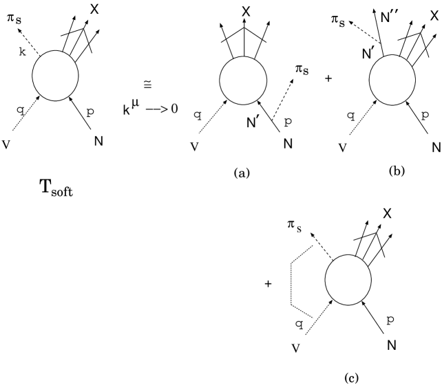
Figure 1: The soft pion theorem in the inclusive reaction. The graph (a) is the one where the proper part of the axial-vector current is attached to the initial nucleon, the graph (b) is the one to the final nucleon (anti-nucleon), and the graph (c) is the one which comes from the null-plane commutator.

The graph (a) is the one where the proper part of the axial-vector current is attached to the initial nucleon. We call the term which comes from this type of the graph as the pion emission from the initial nucleon. The graph (b) is the one where the proper part of the axial-vector current is attached to the final nucleon (anti-nucleon). We call the term which comes from this type of the graph as the pion emission from the final nucleon. The graph (c) is the one which comes from the null-plane commutator. We call the term of this kind as the commutator term. The hadronic tensor can be obtained by squaring this amplitude, and we have several terms corresponding to the three origins in the amplitude. Among them, the term where the one soft pion is attached to the one final nucleon (anti-nucleon) and the other to the initial nucleon or the term where the two soft pions are attached to the different final nucleons can be neglected at high energy. In these cases we have the odd number of the helicity factors in the same nucleon(anti-nucleon) line in the final state arising from the matrix element of the following form $\langle p(p),h|J^{5+}_{a}(0)|n(p),h^{\prime}\rangle=2p^{+}hg_{A}(0)\delta_{hh^{\prime}}$, where $p$ means the proton, $n$ means the neutron, $h$ means the helicity factor, and we take $a=1+i2$ by way of illustration. Since, at high energy, we can expect that the production of the $+$ helicity nucleon (anti-nucleon) and that of the $-$ helicity one are the same order, the contributions from these terms are expected to be small compared with those terms where the helicity factors in the same nucleon(anti-nucleon) line in the final state are even. Typical graphs contributing to the hadronic tensor are given in Fig.2.

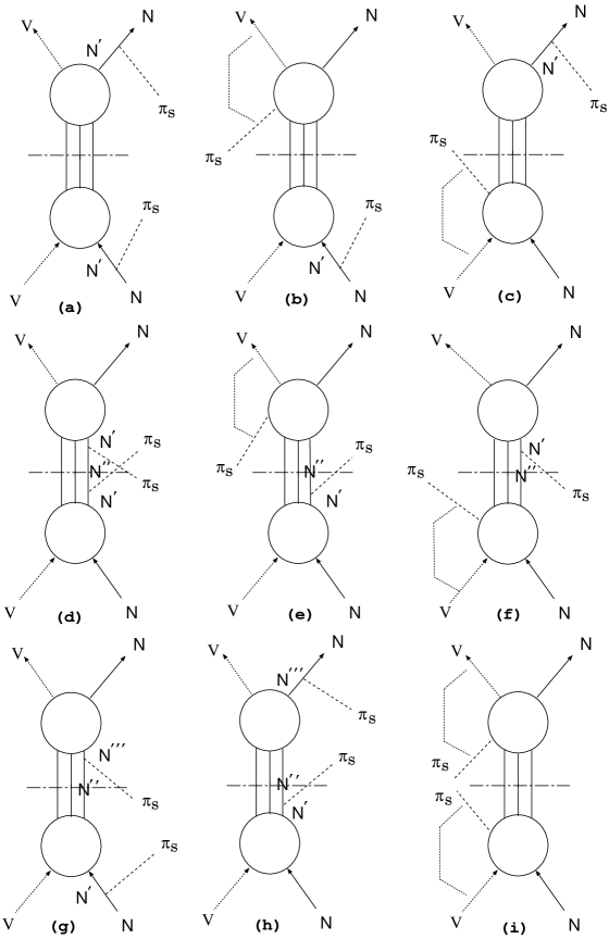
Figure 2: Graphical representation of the soft pion correction for the hadronic tensor.

Thus, among the graphs in Fig.2, we take the contribution from the graphs $(a),(b),(c),(d)$, and $(i)$ into consideration, and discard those from the graphs $(e),(f),(g)$, and $(h)$. Now the contributions from the graphs $(a)$ and $(d)$ are related to the known process directly. Hence, to estimate these, we need no assumption except the one necessary to apply the soft pion theorem. However, to estimate the contribution from the graphs from $(b),(c)$,and $(i)$, we need further theoretical consideration. A detailed explanation to estimate these parts are given in Appendix A.

III Soft pion contribution to the sea quarks

Now we denote the structure functions $F_{2}^{lp(n)}$ where the suffix $l$ means the lepton and $p(n)$ means the proton (the neutron). Further, we define $F_{2}^{\mu N}=\frac{1}{2}(F_{2}^{\mu p}+F_{2}^{\mu n}),$ and $F_{2}^{\nu N}=\frac{1}{4}(F_{2}^{\nu p}+F_{2}^{\nu n}+F_{2}^{\bar{\nu}p}+F_{2}^{\bar{\nu}n}).$ Let us first give the soft pion correction for the differential between the up and the down sea quark distributionkore20 . Since the separation of the sea and the valence part in the up and the down quark distribution has some ambiguity, we use here the Adler sum rule. This sum rule is considered to be exactly satisfied at the structure function level. We require this also at the quark distribution level as is usually fulfilled in a phenomenological analysis. Thus the valence up and down quarks need no correction from the soft pion since they are defined through the experimentally measurable quantity such as the structure function where the soft pion effect is already included. This causes a subtlety in the separation of the up and the down sea quark distribution into the soft pion part and the other one. A detailed explanation of this fact is given in Appendix B. Then, the soft pion correction for $x(\lambda_{d}-\lambda_{u})$ where $\lambda_{i}$ for $i=u,d,s$ denotes the sea quark distribution for each flavor has been determined from the soft pion correction for the structure function $(F_{2}^{ep}-F_{2}^{en})$ as $(F_{2}^{ep}-F_{2}^{en})|_{{\rm soft}}=-2x(\lambda_{d}-\lambda_{u})|_{{\rm soft}}/3$. Here the $\lambda_{d}|_{{\rm soft}}$ and $\lambda_{u}|_{{\rm soft}}$ are $\lambda_{d}|_{{\rm soft}}^{1}$ and $\lambda_{u}|_{{\rm soft}}^{1}$ in Appendix B respectively(see Eqs.(B12) and (B13)). Thus we obtain

$$x(\lambda_{d}-\lambda_{u})|_{{\rm soft}}=\frac{-3I_{\pi}}{8f_{\pi}^{2}}[g_{A}^{2}(0)(F_{2}^{ep}-F_{2}^{en})(3<n>-1)-16xg_{A}(0)(g_{1}^{ep}-g_{1}^{en})].$$ (1)

The various expressions on the right-hand side of this equation are as follows: The mean multiplicity $\langle n\rangle$ is the sum of the nucleon and the anti-nucleon multiplicity, and the factor $I_{\pi}$ is the phase space factor of the soft pion defined as

$$I_{\pi}=\int\frac{d^{2}\vec{k}^{\bot}dk^{+}}{(2\pi)^{3}2k^{+}},$$ (2)

with a kinematical constraint explained later in this section. The spin dependent structure function $g_{1}^{ep(n)}$ is a usual one. For example, $g_{1}^{ep}$ can be expressed as $\displaystyle{\frac{1}{2}\sum[\frac{4}{9}\triangle u+\frac{1}{9}\triangle d+\frac{1}{9}\triangle s]}$, where $\triangle q$ with $q=u,d,s$ is a sum of the quark and the antiquark of the differential between the helicity $+$ distribution and the helicity $-$ one along the direction of the proton spin in the infinite momentum frame in the parton model. The spin-dependent term in Eq.(1) is obtained in the approximation in which the sea quark contribution to $(g_{1}^{ep}-g_{1}^{en})$ is ignored. Without this approximation, $16(g_{1}^{ep}-g_{1}^{en})$ in Eq. (1) should be replaced by $\displaystyle{24(g_{1}^{ep}-g_{1}^{en})-\frac{4}{3}(g_{1}^{\bar{\nu}p}-g_{1}^{\nu p})}$. The graphs in Fig.2 can be identified to the various expressions in Eq.(1) as follows. The term proportional to the $\langle n\rangle$ comes from the graph $(d)$, the term proportional to $g_{A}^{2}(0)$ without the nucleon multiplicity factor comes from the graph $(a)$, and the term proportional to $g_{A}(0)$ comes from the graphs $(b)$ and $(c)$. The contribution from the graph $(i)$ is canceled out by adding the contributions from the $\pi_{s}^{+}$,$\pi_{s}^{-}$, and $\pi_{s}^{0}$.

The soft pion correction for the strange sea quark distribution can be obtained by calculating the soft pion contribution to the structure function $(\frac{5}{6}F_{2}^{\nu N}-3F_{2}^{\mu N})$. In the $SU(4)$ model with the Cabibbo angle being 0 we obtain

$$(\frac{5}{6}F_{2}^{\nu N}-3F_{2}^{\mu N})|_{{\rm soft}}=\frac{I_{\pi}}{f_{\pi}^{2}}[\frac{1}{12}(F_{2}^{\nu p}+F_{2}^{\bar{\nu}p})_{0}+\frac{5}{16}g_{A}^{2}(0)(F_{2}^{\nu p}+F_{2}^{\bar{\nu}p})(1+\langle n\rangle^{\nu N})$$ (3)

$$- \frac{9}{8}(F_{2}^{ep}+F_{2}^{en})g_{A}^{2}(0)(1+\langle n\rangle^{eN})-10xg_{A}(0)(g_{1}^{ep}-g_{1}^{en})].\hskip 113.81102pt$$

Since $(\frac{5}{6}F_{2}^{\nu N}-3F_{2}^{\mu N})$ is expressed as $x(\lambda_{s}-\lambda_{c})$, in the kinematical region where the charm sea quark can be neglected, we can set $(\frac{5}{6}F_{2}^{\nu N}-3F_{2}^{\mu N})=x\lambda_{s}$. The suffix 0 in the expression $(F_{2}^{\nu p}+F_{2}^{\bar{\nu}p})_{0}$ on the right hand side of Eq.(3) means the structure function defined in the $SU(3)$ model, and it comes from the graph $(i)$ in Fig.2. The reason why we meet here such structure functions is as follows. The flavor suffix of the axial-vector current corresponding to the pion is $1\pm i2$ or $3$. We use the commutation relation on the null-plane between the hadronic weak currents and the axial-vector current, hence the part related to the strange sea quark and the charm sea quark in the weak hadronic current drops out in this step. The structure function obtained after such a manipulation is equivalent to the structure function in the $SU(3)$ model with the Cabibbo angle being 0. Thus in the kinematical region where the charm sea quark contribution is neglected we obtain

$$x\lambda_{s}|_{{\rm soft}}=\frac{I_{\pi}}{f_{\pi}^{2}}[\frac{x}{6}(d_{v}+u_{v})+\frac{x}{3}(\lambda_{u}+\lambda_{d})+\frac{3}{4}xg_{A}^{2}(0)(1+\langle n\rangle)\lambda_{s}$$ (4)

$$-\frac{5}{3}xg_{A}(0)(\triangle u_{v}-\triangle d_{v})],$$

where we set $\langle n\rangle^{\nu N}=\langle n\rangle^{eN}=\langle n\rangle$, and the $\triangle u_{v}$($\triangle d_{v}$) is the valence part in the $\triangle u$($\triangle d$). Now both hand sides of Eq.(3) get contribution from the charm sea quark. The equation which does not neglect the charm sea quark contribution is the one where the $\lambda_{s}|_{{\rm soft}}$ on the left-hand side of Eq.(4) is simply replaced by the $(\lambda_{s}-\lambda_{c})|_{{\rm soft}}$ and the $\lambda_{s}$ on the right-hand side of it by the $(\lambda_{s}-\lambda_{c})$. Since the main contribution in the small $x$ region comes from the term proportional to the factor $(1+\langle n\rangle)$ and the charm sea quark begins to contribute also in this region, the additional parts which is added to both hands side of Eq.(4) can be equated as

$$x\lambda_{c}|_{{\rm soft}}=\frac{I_{\pi}}{f_{\pi}^{2}}\left[\frac{3}{4}xg_{A}^{2}(0)(1+\langle n\rangle)\lambda_{c}\right].$$ (5)

With this assumption, we regard Eq.(4) as the formula to determine the soft pion contribution to the strange sea quark distribution even in the region where the charm sea quark contribution can not be neglected. Now, following Eqs.(B12) and (B13) in Appendix B, we have the relation $F_{2}^{\nu N}|_{{\rm soft}}=2x(\lambda_{u}|_{{\rm soft}}+\lambda_{d}|_{{\rm soft}}+\lambda_{s}|_{{\rm soft}}+\lambda_{c}|_{{\rm soft}})$, where $\lambda_{u}|_{{\rm soft}}=\lambda_{u}|_{{\rm soft}}^{1}$ and $\lambda_{d}|_{{\rm soft}}=\lambda_{d}|_{{\rm soft}}^{1}$ as is already stated. The soft pion correction for the $F_{2}^{\nu N}|_{{\rm soft}}$ can be calculated as

$$F_{2}^{\nu N}|_{{\rm soft}}=\frac{I_{\pi}}{f_{\pi}^{2}}[2(F_{2}^{\nu N})_{0}+\frac{3}{4}g_{A}^{2}(0)(1+\langle n\rangle)F_{2}^{\nu N}-12xg_{A}(0)(g_{1}^{ep}-g_{1}^{en})],$$ (6)

where the suffix 0 in the expression $(F_{2}^{\nu N})|_{0}$ means the structure function in the $SU(3)$ model as in Eq.(3). Thus, using Eqs.(1),(4),(5) and (6) we obtain

$$x\lambda_{u}|_{{\rm soft}}=\frac{I_{\pi}}{f_{\pi}^{2}}[\frac{5x}{12}(d_{v}+u_{v})+\frac{5x}{6}(\lambda_{u}+\lambda_{d})+\frac{x}{8}g_{A}^{2}(0)(1+3\langle n\rangle)u_{v}+\frac{x}{4}g_{A}^{2}(0)d_{v}$$ (7)

$$-\frac{x}{6}g_{A}(0)(\triangle u_{v}-\triangle d_{v})+\frac{1}{4}xg_{A}^{2}(0)(1+3\langle n\rangle)\lambda_{u}+\frac{1}{2}xg_{A}^{2}(0)\lambda_{d}],$$

$$x\lambda_{d}|_{{\rm soft}}=\frac{I_{\pi}}{f_{\pi}^{2}}[\frac{5x}{12}(d_{v}+u_{v})+\frac{5x}{6}(\lambda_{u}+\lambda_{d})+\frac{x}{8}g_{A}^{2}(0)(1+3\langle n\rangle)d_{v}+\frac{x}{4}g_{A}^{2}(0)u_{v}$$ (8)

$$+\frac{5x}{6}g_{A}(0)(\triangle u_{v}-\triangle d_{v})+\frac{1}{4}xg_{A}^{2}(0)(1+3\langle n\rangle)\lambda_{d}+\frac{1}{2}xg_{A}^{2}(0)\lambda_{u}].$$

Let us now consider the phase space factor $I_{\pi}$. We assume the soft pion satisfies the following two conditions:

(1)

The transverse momentum satisfies $|\vec{k}^{\bot}|\leq bm_{\pi}$.

(2)

Feynman scaling variable $x_{F}=2k^{3}/\sqrt{s}$ satisfies $|x_{F}|\leq c$, where $s=(p+q)^{2}$.

Then, $I_{\pi}$ at high energy can be calculated explicitly as

$$I_{\pi} = \frac{1}{16\pi^{2}}\Bigg{(}(b^{2}+1)m_{\pi}^{2}\log\left(\frac{\sqrt{(1+b^{2})m_{\pi}^{2}+\frac{c^{2}s}{4}}+\frac{c\sqrt{s}}{2}}{\sqrt{(1+b^{2})m_{\pi}^{2}+\frac{c^{2}s}{4}}-\frac{c\sqrt{s}}{2}}\right)$$

$$- m_{\pi}^{2}\log\left(\frac{\sqrt{m_{\pi}^{2}+\frac{c^{2}s}{4}}+\frac{c\sqrt{s}}{2}}{\sqrt{m_{\pi}^{2}+\frac{c^{2}s}{4}}-\frac{c\sqrt{s}}{2}}\right)+c\sqrt{s}\left(\sqrt{(1+b^{2})m_{\pi}^{2}+\frac{c^{2}s}{4}}-\sqrt{m_{\pi}^{2}+\frac{c^{2}s}{4}}\right)\Bigg{)}.$$

Following the previous studykore98 ; kore20 , we set $b=1$ and $c=0.1$. Though a large ambiguity exists here, these are the parameters which explain the pion charge asymmetry in the central region with low transverse momentum in the experimentBebek fairly wellkore78reso ; kore82 , and gave an adequate quantity required by the Gottfried defectkore98 . Of course these parameters should be determined more accurately. For example, the energy dependence of the parameter $c$ should be studied by the high energy experiment such as a pion charge asymmetry measurement in the central region with the low transverse momentum. Now as to the mean multiplicity $\langle n\rangle$, We take $\langle n\rangle=1+a\log(s)$. The parameter $a$ is fixed as 0.21 in consideration of the (nucleon + anti-nucleon) multiplicity in the $e^{+}e^{-}$ annihilation such that $a\log\sqrt{s}$ with $\sqrt{s}$ replaced by the CM energy of that reaction agrees with the multiplicity of that reactionDELPHI . Now we can check the magnitude of the soft pion correction for the sea quarks if we specify the input distributions which can be used on the right hand side of Eqs.(4),(7),and (8). The exact magnitude of the soft pion correction greatly depends on this input. Let us first estimate the various terms by using typical sea quark distributions given in Ref.GS at $Q_{0}^{2}=4{\rm GeV}^{2}$.

Figure 3: A typical example of the soft pion correction for the down sea quark distribution $x\lambda_{d}$ and the strange sea quark distribution $x\lambda_{s}$. The soft pion correction for $x\lambda_{d}$ is decomposed into three types. XDBAR_1(x) is the contribution from the valence quark, XDBAR_2(x) is the one from the sea quark from the graph (a) and (i) in Fig.2, and XDBAR_3(x) is the one from the sea quark from the graph (d) in Fig.(2)

In FIG.3, the contribution to the $x\lambda_{d}|_{\rm soft}$ decomposed into the three types are given. The XDBAR_1(x) is the one from the valence quarks coming from all the graphs considered in Fig.(2). The XDBAR_2(x) is the one from the sea quark coming from the graph $(a)$ and $(i)$ in Fig.2. The XDBAR_3(x) is the one from the sea quark coming from the graph $(d)$ in Fig.2. The estimate given in Fig.3 is overestimate since the phenomenologically determined quark distribution already includes the soft pion correction, and the distributions on the right hand side of Eqs.(4),(7),and (8) should be the ones without the soft pion correction. However, as far as its correction is small, we can discard this fact and study its magnitude roughly. In the region above $x\sim 0.1$, the soft pion corrections are dominated by the terms originating from the valence quarks and its magnitude is large in the up and the down sea quark distribution. On the other hand, the correction for the strange sea quark distribution is greatly suppressed in this region. This reflects the fact that the contribution from the commutator terms is suppressed. Below the region $x\sim 0.1$, the corrections originating from the sea quarks begin to become large and they take over the ones from the valence quarks. They come both from the pion emission terms and the commutator term. In accord with this, the correction for the strange sea quark distribution begins to become sizable. We find that the correction from the soft pion for the strange sea quark distribution is yet suppressed, but near the region $x\sim 0.01$, its magnitude becomes about 1/3 of the correction for the up or the down sea quark one. In the region below $x\sim 0.01$, among the above terms the pion emission from the final nucleon(anti-nucleon) term being proportional to $\langle n\rangle$ begins to become very large, and, in the region below $x\sim 0.001$, its magnitude rapidly becomes dominant one. Thus in the region below $x\sim 0.01$, by keeping the contribution only from the sea quark, the soft pion correction to the down sea quark distribution can be set effectively as

$$x\lambda_{d}|_{\rm soft}=\frac{I_{\pi}}{f_{\pi}^{2}}[\frac{5x}{3}\lambda_{d}+\frac{3}{4}xg_{A}^{2}(0)(1+\langle n\rangle)\lambda_{d}],$$ (10)

where we set $x\lambda_{u}=x\lambda_{d}$ because, in this small $x$ region, the differential between the up and the down sea quark distribution is very small compared with their sum. Further we set $x\lambda_{d}|_{\rm soft}=x\lambda_{u}|_{\rm soft}$ by this same reason. Similarly, the strange sea qaurk distribution can be set as

$$x\lambda_{s}|_{\rm soft}=\frac{I_{\pi}}{f_{\pi}^{2}}[\frac{2x}{3}\lambda_{d}+\frac{3}{4}xg_{A}^{2}(0)(1+\langle n\rangle)\lambda_{s}].$$ (11)

It should be noted that the distinction of the sea quark distributions classified by the superscript 0 and 1 discussed in Appendix B does not matter since both give the same result (10). This is because the differential between the two definitions lies in the soft pion correction to the valence quark distribution and it is given only by the valence quark distributions.

IV The behavior of the soft pion correction in the small $x$ region

Now the distribution on the right hand side of Eqs.(4),(7),and (8) should be the ones without the soft pion correction as is already noted. We can discard this fact as far as the soft pion correction is small as in the case of the differential of the up and the down sea quark distributions in the modified Gottfried sum rule. However, when it comes to the sea quark distribution itself, we must take into account this fact since its correction is large in the small $x$ region. Here we consider this by using Eqs.(10) and (11). In the approximation to neglect the higher order soft pion corrections, we can express the phenomenologically determined sea qaurk distribution $x\lambda_{i}|_{\rm ph}$ for $i=u,d,s$ as $\lambda_{i}|_{\rm ph}=\lambda_{i}|_{\rm ns}+\lambda_{i}|_{\rm soft}$, where the distribution $x\lambda_{i}|_{\rm ns}$ is the one with no soft pion. In this case the $x\lambda_{d}$ and $x\lambda_{s}$ on the right hand side of Eqs.(10) and (11) should be $x\lambda_{d}|_{\rm ns}$ and $x\lambda_{s}|_{\rm ns}$ respectively. Then it may be thought that even if $x\lambda_{d}|_{\rm ns}$ and $x\lambda_{s}|_{\rm ns}$ becomes symmetric in the very small $x$ region the soft pion correction is asymmetric because of the difference between the first term on the right hand side of Eq.(10) and that of Eq.(11). This is not the case if a certain condition is satisfied as discussed below. Let us first assume $x\lambda_{d}|_{\rm ns}$ and $x\lambda_{s}|_{\rm ns}$ becomes symmetric somewhere in the very small $x$ region. We call the terms proportional to $g_{A}^{2}(0)$ on the right hand side of Eqs.(10) and (11) as symmetric terms, and the rest as the commutator terms since they come from the graph (i) in Fig.2. In the small $x$ region, Eq.(10) and the definition of the phenomenologically determined distribution $\lambda_{d}|_{\rm ph}$ gives us the relation $x\lambda_{d}|_{\rm ns}=x\lambda_{d}|_{\rm ph}/(1+K_{d})$ with $K_{d}=\frac{I_{\pi}}{f_{\pi}^{2}}(\frac{5}{3}+\frac{3g_{A}^{2}(0)}{4}(1+\langle n\rangle))$. Since $\langle n\rangle$ becomes very large as $x\to 0$, $x\lambda_{d}|_{\rm ns}$ behaves as $x\lambda_{d}|_{\rm ns}\sim x\lambda_{d}|_{\rm ph}/(\langle n\rangle I_{\pi})$ apart from a numerical factor. Thus the commutator term in Eq.(10) behaves as $x\lambda_{d}|_{\rm ph}/\langle n\rangle$, while the rest as $x\lambda_{d}|_{\rm ph}(\langle n\rangle+1)/\langle n\rangle$. Thus if the condition

$$\lim_{x\to 0}\frac{x\lambda_{d}|_{\rm ph}}{\langle n\rangle}=0,$$ (12)

is satisfied, the commutator term being asymmetric vanishes and, among the remaining symmetric term, the one which comes from the pion emission from the final nucleon(anti-nucleon) remains. The important point is that this fact does not depend on the soft pion phase space factor. At small $Q^{2}\sim 1$ GeV², the experiment at HERA shows that the behavior of the structure function in the small $x$ region is like the soft pomeron. Though the nucleon multiplicity is assumed to behave as $\log(s)$ in this paper, it can be also parameterized as if it behaves like $s^{0.15}$, and we cannot distinguish between these two casesDELPHI . Thus the Eq.(12) have a good chance to be satisfied. Even if it is not satisfied, the contribution from the commutator term becomes far smaller than that from the pion emission terms as we go to the smaller $x$ region. Thus the multi-soft pion effect from the pion emission from the nucleon(anti-nucleon) in the final state enhances the symmetric term and the commutator term becomes negligible. In this way, we can understand why the soft pion correction for the sea quark distribution becomes $SU(3)$ flavor symmetric. Now the $SU(3)$ flavor symmetry in the limit $x\to 0$ is the necessary condition for the mean charge sum rule which holds under the same theoretical basis with the modified Gottfried sum rule. It takes the form

$$\int_{0}^{1}dx\{\frac{2}{3}\lambda_{u}-\frac{1}{3}\lambda_{d}-\frac{1}{3}\lambda_{s}\}\sim 0.2.$$ (13)

This sum rule is $Q^{2}$ independent and the perturbative correction is negligibly small as in the modified Gottfried sum rule. On the one hand the soft pion correction for the strange sea quark distribution has a phenomenologically favorable property being suppressed in the large and the medium $x$ region, but on the other hand it can have a theoretically favorable property being symmetric in the very small $x$ region. Since the sum rule is very sensitive about the way how the symmetry of the strange sea quark distribution is restored in the small $x$ regionkore98 ; kore21 , let us study the sea quark distributions at $Q^{2}\sim 1$ GeV² quantitably by using this sum rule. Since the sea quark distributions above $x=0.01$ can be expected to be relatively well determined phenomenologically, we use, for example, the distributions given by MRSTMRST in this region and find that it takes the value about 0.03. Then,below $x=0.01$, we consider that $x\lambda_{d}|_{\rm ns}$ is determined through Eq.(10) as $x\lambda_{d}|_{\rm ns}=x\lambda_{d}|_{\rm ph}/(1+K_{d})$, where we use $x\lambda_{d}|_{\rm ph}$ as the one given by MRST. By setting $x\lambda_{s}|_{\rm ns}=x\lambda_{d}|_{\rm ns}/2$ at $x=0.01$, we take the interpolating function as $I(x)=1.085\exp[156.6x-5848x^{2}-17.65\sqrt{x}]$, and set $\lambda_{s}|_{\rm ns}=I(x)\lambda_{d}|_{\rm ns}$ from $x=0.01$ up to $x=10^{-6}$, and determine the $x\lambda_{s}|_{\rm ph}$ by using Eq.(11) as $x\lambda_{s}|_{\rm ph}=x\lambda_{s}|_{\rm ns}+x\lambda_{s}|_{\rm soft}$. The interpolating function is constructed to ensure that the strange sea quark distribution determined in this way can be continued to the one of the MRST at $x=0.01$, and that near $x=10^{-6}$ it becomes almost symmetric as is seen in Fig.4. Then, below $x=0.01$, using this strange sea quark distribution together with the MRST distribution for the down and the up sea quark distributions we find that their contribution to the sum rule is about 0.19, where the contribution below $x=10^{-6}$ is set zero by regarding the sea quark distribution being $SU(3)$ flavor symmetric in this region. Thus combining the value above $x=0.01$, the sum rule takes the value about 0.22. Though the extrapolation is rather arbitrary, we should see the behavior of the strange sea quark distribution in the region from $x=10^{-2}$ to $10^{-6}$. If we use the MRST sea quark distributions even for the strange sea quark one in the sum rule (13), their contribution to it in this region is 0.72. Thus the sum rule is badly broken already in this region.

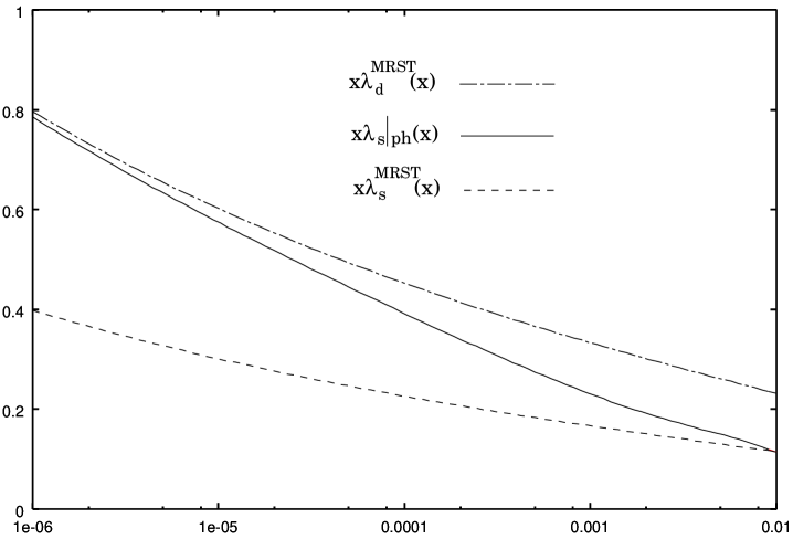
Figure 4: The strange sea quark distribution $x\lambda_{s}|_{\rm ph}$ together with the down and the strange sea quark distribution $x\lambda_{d}^{MRST}$ and $x\lambda_{s}^{MRST}$ given by MRST,MRST where the $x\lambda_{d}^{MRST}$ is identified as the down sea quark distribution $x\lambda_{d}|_{\rm ph}$ in the analysis in sect.IV.

V Conclusion

The soft pion may contribute to the experimentally measured quantity even at high energy. If this is the case, we must either subtract the soft pion effect from the experimental data or include it in the parameters of the theoretical model considered. In this paper, we have shown that, while the soft pion correction for the strange sea quark distribution is suppressed in the large and the medium $x$ region, it becomes $SU(3)$ flavor symmetric in the very small $x$ region somewhere below $x\sim 0.01$. Based on this fact, by interpolating the asymmetric strange sea quark distribution to the symmetric one, the mean charge sum rule for the light sea quark which holds under the same theoretical basis with the modified Gottfried sum rule has been studied. This sum rule requires the symmetric light sea quark distributions in the limit $x\to 0$. However, there was no theoretical reason why the strange sea quark distribution being suppressed in the large $x$ region became large and flavor symmetric in the very small $x$ region. The soft pion correction has these properties. Moreover, the sum rule is very sensitive about the way how the symmetry of the strange sea quark distribution is restored. Then, by estimating the sum rule, it has been discussed that the large symmetry restoration of the light sea quarks originating from the soft pion emission from the nucleon(antinucleon) in the final state should exist in the region from $x=10^{-2}$ to $10^{-6}$ at $Q^{2}\sim 1$ GeV.

Appendix A

The hadronic tensor of the reaction $V^{\mu}(q)+N(p)\to\pi_{s}(k)+anythings(X_{0})$kore78 can be expressed as

$$T^{\mu\nu}_{abcd}=(m_{\pi}^{2}-k^{2})^{2}\int d^{4}xd^{4}yd^{4}z\exp[-ik\cdot(x-z)+iq\cdot y]$$

$$\times \langle N(p)|[T^{\dagger}(\phi_{\pi}^{a^{\prime}}(x)V^{\mu}_{b^{\prime}}(y)),T(\phi_{\pi}^{c}(z)V^{\nu}_{d}(0))]|N(p)\rangle_{c},$$ (14)

where the spectral condition is used to express the tensor as the matrix element of the commutator, $a^{\prime\dagger}=a,b^{\prime\dagger}=b$, and the sum over the intermediate state $X_{0}$ is understood. Then we define the soft pion limit of the hadronic tensor as $W^{\mu\nu}_{abcd}(p,q)$, where we neglect the argument $k$ since the limit $k^{\mu}\to 0$ is taken. Under the exchange $q\to-q$ and $a\leftrightarrow c,b\leftrightarrow d$, the each structure function defined by the hadronic tensor has a definite crossing property. Among the terms in $W^{\mu\nu}_{abcd}(p,q)$, the term coming from the graph (b) in Fig.2 is given, for example, as

$$A^{\mu\nu}_{2}=\frac{-1}{4f_{\pi}^{2}p^{+}}\int d^{4}x\int d^{4}y\exp(iq\cdot y)\delta(x^{+}-y^{+})$$

$$\times \{\langle N(p)|[J_{a}^{5+}(x),V_{b}^{\mu}(y)]V_{d}^{\nu}(0)|N^{\prime}(p)\rangle\langle N^{\prime}(p)|J_{c}^{5+}(0)|N(p)\rangle$$

$$+ \langle N(p)|J_{c}^{5+}(0)|N^{\prime}(p)\rangle\langle N^{\prime}(p)|V_{d}^{\nu}(0)[J_{a}^{5+}(x),V_{b}^{\mu}(y)]|N(p)\rangle\}.$$ (15)

If we set $a=1+i2,c=1-i2,$ and $b=d^{\dagger}$ and take the target as the proton, the second term in the brace on the right hand side of Eq.(A2) is zero. While, by taking $\mu=\nu=+$ and using the current commutation relation on the null-plane, the first term becomes the product of the currents if we replace the sum over the intermediate state $X_{0}$ to the complete set of the state. We can not change this product to the commutation relation which may be obtained as the imaginary part of the retarded product, since it changes the crossing property. Thus we must use the method which can be applied directly to the light-cone dominated process such as the cut vertex formalismMue . Further this example shows that the quantity which we must calculate is the nucleon matrix element of the currents product, hence we see that this part is related to the structure function in the total inclusive reactions. For the purpose of searching such a relation, we can use the light-cone current algebrafg at some $Q^{2}=Q_{0}^{2}$. We take this as the point where the perturbative evolution is started. Now we encounter the symmetric bilocal current and the antisymmetric one. The nucleon matrix element of these currents distinguish how the quark and the antiquark contribute. Let us explain this fact in details.

We define

$$W^{\mu\nu}_{ab}=\frac{1}{4\pi M}\int d^{4}x\exp[iq\cdot x]\langle N(p)|J_{a}^{\mu}(x)J_{b}^{\nu}(0)|N(p)\rangle_{c}.$$ (16)

In the light-cone limit $q^{-}\to\infty$, the leading term comes from the region $x^{+}=0$ and $x^{2}=0$. Hence we take $\vec{x}^{\bot}=0$ but $x^{-}$ is left arbitrary. Using the light-cone current algebra, we see that $F_{2}$ is proportional to $\eta\widetilde{F}_{ab}(\eta)$ with $\eta=-q^{2}/2p\cdot q$ and $\widetilde{F}_{ab}(\eta)$ being defined as

$$F_{ab}(p\cdot x,x^{2}=0)=\int d\eta\exp[i\eta p\cdot x]\tilde{F}_{ab}(\eta),$$ (17)

where $F_{ab}(p\cdot x,x^{2})$ is defined as

$$\langle N(p)|F_{ab}^{\mu}(x|0)|N(p)\rangle_{c}=p^{\mu}F_{ab}(p\cdot x,x^{2})+x^{\mu}\bar{F}_{ab}(p\cdot x,x^{2}).$$ (18)

The bilocal currents $F_{ab}^{\mu}(x|0)$ is decomposed into the symmetric and the antisymmetric bilocal as $F_{ab}^{\mu}(x|0)=f_{abc}S_{c}^{\mu}(x|0)+d_{abc}A_{c}^{\mu}(x|0)$, where

$$S_{c}^{\mu}(x|0) = \frac{1}{2}\{:\bar{q}(x)\gamma^{\mu}\frac{\lambda_{c}}{2}q(0)+\bar{q}(0)\gamma^{\mu}\frac{\lambda_{c}}{2}q(x):\},$$

$$A_{c}^{\mu}(x|0) = \frac{1}{2i}\{:\bar{q}(x)\gamma^{\mu}\frac{\lambda_{c}}{2}q(0)-\bar{q}(0)\gamma^{\mu}\frac{\lambda_{c}}{2}q(x):\}.$$ (19)

Here the phase factor is discarded by taking the light cone gauge$A^{+}=0$ for simplicity, but the following discussion is unchanged if we do not take this gauge and include it. Corresponding to the decomposition of the symmetric and antisymmetric bilocals, we define $\widetilde{F}_{ab}(\eta)=f_{abc}S_{c}(\eta)+d_{abc}A_{c}(\eta)$. Now we expand the quark field on the null-plane $x^{+}=0,\vec{x}^{\bot}=0$ into the creation and the annihilation operator as

$$q(x)=\sum_{n}a_{n}\phi_{n}^{(+)}(x)+\sum_{n}b_{n}^{\dagger}\phi_{n}^{(-)}(x),$$ (20)

where the sum over the subscript $n$ means the spin sum and the momentum integral collectively. Here $(+)$ means the positive energy solution and $(-)$ the negative one. The normal ordered product is given as

$$:\bar{q}(x)\gamma^{+}\frac{\lambda_{a}}{2}q(0):=\sum_{n,m}a_{n}^{\dagger}a_{m}\bar{\phi}_{n}^{(+)}(x)\gamma^{+}\frac{\lambda_{a}}{2}\phi_{m}^{(+)}(0)-\sum_{n,m}b_{m}^{\dagger}b_{n}\bar{\phi}_{n}^{(-)}(x)\gamma^{+}\frac{\lambda_{a}}{2}\phi_{m}^{(-)}(0).$$ (21)

Then, when the matrix $\lambda_{a}/2$ is diagonal, we define a part contributing to the quark distribution function of the proton as

$$<a>f_{a}(x)=\frac{1}{2\pi p^{+}}\int_{-\infty}^{\infty}d\alpha\exp[-ix\alpha]\langle p|\sum_{n,m}a_{n}^{\dagger}a_{m}\bar{\phi}_{n}^{(+)}(y^{-})\gamma^{+}\frac{\lambda_{a}}{2}\phi_{m}^{(+)}(0)|p\rangle_{c},$$ (22)

and a part contributing to the antiquark one as

$$<\bar{a}>g_{\bar{a}}(x)=-\frac{1}{2\pi p^{+}}\int_{-\infty}^{\infty}d\alpha\exp[-ix\alpha]\langle p|\sum_{n,m}b_{m}^{\dagger}b_{n}\bar{\phi}_{n}^{(-)}(0)\gamma^{+}\frac{\lambda_{a}}{2}\phi_{m}^{(-)}(y^{-})|p\rangle_{c},$$ (23)

where $\alpha=p^{+}y^{-}$, $<a>$ is a symmetry factor originating from the flavor symmetry, and $<\bar{a}>=-<a>$. Here we use an abbreviated notation. For example, when $a=3$, $\displaystyle{<a>f_{a}=\frac{1}{2}f_{u}-\frac{1}{2}f_{d}}$ and $\displaystyle{<\bar{a}>g_{\bar{a}}=-\frac{1}{2}g_{\bar{u}}+\frac{1}{2}g_{\bar{d}}}$. Corresponding to the decomposition of the normal ordered product, we classify the matrix element of the bilocal current into the quark part and the antiquark part as

$$S_{a}(\alpha)=S_{a}^{q}(\alpha)+S_{a}^{\bar{q}}(\alpha),\qquad A_{a}(\alpha)=A_{a}^{q}(\alpha)+A_{a}^{\bar{q}}(\alpha).$$ (24)

The moments becomes

$$\int_{0}^{\infty}dxx^{n-1}<a>f_{a}(x)=\frac{(n-1)!(-i)^{n}}{2\pi p^{+}}$$

$$\times \int_{-\infty}^{\infty}d\alpha\frac{1}{(\alpha-i\epsilon)^{n}}\langle p|\sum_{n,m}a_{n}^{\dagger}a_{m}\bar{\phi}_{n}^{(+)}(y^{-})\gamma^{+}\frac{\lambda_{a}}{2}\phi_{m}^{(+)}(0)|p\rangle_{c},$$ (25)

and

$$\int_{0}^{\infty}dxx^{n-1}<\bar{a}>g_{\bar{a}}(x)=\frac{-(n-1)!(i)^{n}}{2\pi p^{+}}$$

$$\times \int_{-\infty}^{\infty}d\alpha\frac{1}{(\alpha+i\epsilon)^{n}}\langle p|\sum_{n,m}b_{m}^{\dagger}b_{n}\bar{\phi}_{n}^{(-)}(y^{-})\gamma^{+}\frac{\lambda_{a}}{2}\phi_{m}^{(-)}(0)|p\rangle_{c}.$$ (26)

Then, using the facts $:\bar{q}(x)\gamma^{\mu}\frac{\lambda_{a}}{2}q(0):=S_{a}^{\mu}+iA_{a}^{\mu}$ and the support property of the quark distribution function we obtain

$$\int_{0}^{1}dxx^{n-1}<a>f_{a}(x)=\frac{(n-1)!(-i)^{n}}{2\pi}\int_{-\infty}^{\infty}d\alpha\frac{1}{(\alpha-i\epsilon)^{n}}[S_{a}^{q}(\alpha)+iA_{a}^{q}(\alpha)],$$ (27)

and

$$\int_{0}^{1}dxx^{n-1}<\bar{a}>g_{\bar{a}}(x)=\frac{(n-1)!(-i)^{n}}{2\pi}\int_{-\infty}^{\infty}d\alpha\frac{1}{(\alpha-i\epsilon)^{n}}[S_{a}^{\bar{q}}(\alpha)-iA_{a}^{\bar{q}}(\alpha)],$$ (28)

where $S_{a}^{\bar{q}}(-\alpha)=S_{a}^{\bar{q}}(\alpha)$ and $A_{a}^{\bar{q}}(-\alpha)=-A_{a}^{\bar{q}}(\alpha)$ are used to obtain the last equation. Similar equation can be obtained for the normal ordered product $:\bar{q}(0)\gamma^{+}\frac{\lambda_{a}}{2}q(x):$ and we obtain,

$$\int_{-1}^{0}dxx^{n-1}<a>f_{a}(x)=(-1)^{n-1}\int_{0}^{1}dxx^{n-1}<a>f_{a}(-x)$$

$$=\frac{(-1)^{n-1}(n-1)!(-i)^{n}}{2\pi}\int_{-\infty}^{\infty}d\alpha\frac{1}{(\alpha-i\epsilon)^{n}}[S_{a}^{q}(\alpha)-iA_{a}^{q}(\alpha)],$$ (29)

and

$$\int_{-1}^{0}dxx^{n-1}<\bar{a}>g_{\bar{a}}(x)=(-1)^{n-1}\int_{0}^{1}dxx^{n-1}<\bar{a}>g_{\bar{a}}(-x)$$

$$=\frac{(-1)^{n-1}(n-1)!(-i)^{n}}{2\pi}\int_{-\infty}^{\infty}d\alpha\frac{1}{(\alpha-i\epsilon)^{n}}[S_{a}^{\bar{q}}(\alpha)+iA_{a}^{\bar{q}}(\alpha)].$$ (30)

Then, since we have the relation

$$\frac{(-1)^{(n-1)}(n-1)!}{(\alpha-i\epsilon)^{n}}=\frac{d^{n-1}}{d\alpha^{n-1}}\left(\frac{1}{(\alpha-i\epsilon)}\right)=(-1)^{(n-1)}(n-1)!P\frac{1}{\alpha^{n}}+i\pi\delta^{n-1}(\alpha),$$ (31)

at $n=even$, we obtain

$$<a>\int_{0}^{1}dxx^{n-1}[\{f_{a}(x)+f_{a}(-x)\}-\{g_{\bar{a}}(x)+g_{\bar{a}}(-x)]$$

$$=\frac{(n-1)!(-i)^{n}}{\pi}P\int_{-\infty}^{\infty}d\alpha\frac{1}{\alpha^{n}}S_{a}(\alpha),$$ (32)

$$<a>\int_{0}^{1}dxx^{n-1}[\{f_{a}(x)-f_{a}(-x)\}+\{g_{\bar{a}}(x)-g_{\bar{a}}(-x)]$$

$$=i^{n}\int_{-\infty}^{\infty}d\alpha\delta^{n-1}(\alpha)A_{a}(\alpha),$$ (33)

and at $n=odd$

$$<a>\int_{0}^{1}dxx^{n-1}[\{f_{a}(x)+f_{a}(-x)\}-\{g_{\bar{a}}(x)+g_{\bar{a}}(-x)]$$

$$=i^{n-1}\int_{-\infty}^{\infty}d\alpha\delta^{n-1}(\alpha)S_{a}(\alpha),$$ (34)

$$<a>\int_{0}^{1}dxx^{n-1}[\{f_{a}(x)-f_{a}(-x)\}+\{g_{\bar{a}}(x)-g_{\bar{a}}(-x)]$$

$$=\frac{(n-1)!(-i)^{n-1}}{\pi}P\int_{-\infty}^{\infty}d\alpha\frac{1}{\alpha^{n}}A_{a}(\alpha).$$ (35)

Eqs.(A19) and (A22) correspond to the moments of the missing integers in the classical derivation of the moment sum rule and that they are expressed by the nonlocal quantity. Information of these missing parts are supplied by the cut vertex formalism. The moment at $n=1$ stands on a particular status, since we have another method to get information of it. This method is very general. It is independent of the light-cone limit and needs no particular form of the currents. For a detail of this method and the definition of the quark distributions in this method see Ref.kore93 ; kore-ichep and the paper cited therein. As it is explained there, the moments of the structure functions at $n=1$ can be decomposed into the expressions which can be regarded as the moments of the quark distribution functions at $n=1$. The mean charge sum rule discussed in this paper is one example obtained by this method and it holds at any $Q^{2}$. The reason why we obtain the moments like (A19) and (A22) lies in the fact that the current product decomposes into the commutator and the anticommutator. Hence we have the structure function defined by the current commutator and the one by the current anticommutator. They are identically the same in the $s$ channel but opposite in sign in the $u$ channel. Thus the crossing property is opposite. In terms of the quark distribution, this appears as $\int_{-1}^{1}dxx^{n-1}f_{a}(x)$ and $\int_{-1}^{1}dxx^{n-1}\epsilon(x)f_{a}(x)$, where $\epsilon(x)$ is a sign function, and explains why we have two moments for each $n$. The fact is important when we consider the analytical continuation to the complex $n$ plane to obtain the anomalous dimension in the missing integer in the classical derivationRS ; kore83 . Finally, we see that the (quark - antiquark) and the (quark + antiquark) corresponds to the symmetric bilocal and the antisymmetric bilocal respectively. We know that the two different combinations of the quark and the antiquark evolve differentlyRS ; CFP , hence the distinction of these two bilocals is important . However, under the approximation to neglect the sea quark which is equivalent to neglect the antiquark, we need not distinguish the symmetric and antisymmetric bilocals.

Appendix B

Let us consider how the soft pion contribution enters into the correction to $1/3$ in the Gottfried sum. In the parton model, we have

$$x(\lambda_{\bar{d}}-\lambda_{\bar{u}})=-\frac{1}{4}(F_{2}^{\nu p}-F_{2}^{\bar{\nu}p})-\frac{3}{2}(F_{2}^{ep}-F_{2}^{en}).$$ (36)

Thus we can obtain the soft pion contribution to the distribution $x(\lambda_{\bar{d}}-\lambda_{\bar{u}})$ by calculating the soft pion contribution to the structure function $(F_{2}^{\nu p}-F_{2}^{\bar{\nu}p})$ in addition to the structure function $(F_{2}^{ep}-F_{2}^{en})$. Then we can express

$$x(\lambda_{\bar{d}}-\lambda_{\bar{u}})=x(\lambda_{\bar{d}}-\lambda_{\bar{u}})|_{\rm bare}^{0}+x(\lambda_{\bar{d}}-\lambda_{\bar{u}})|_{\rm soft}^{0},$$ (37)

where the superscript 0 distinguish the difference of the definition of the sea quark distribution as explained below and the suffix bare means the contribution other than the soft pion one in this case. The valence part is determined by the Adler sum rule, and we express it as

$$x(u_{v}-d_{v})=x(u_{v}-d_{v})|_{\rm bare}+x(u_{v}-d_{v})|_{\rm soft},$$ (38)

where

$$x(d_{v}-u_{v})|_{\rm soft}=\frac{1}{2}(F_{2}^{\nu p}-F_{2}^{\bar{\nu}p})|_{\rm soft}.$$ (39)

The Adler sum rule determines $\int_{0}^{1}dx\{u_{v}(x)-d_{v}(x)\}=1$. Now, the structure function $(F_{2}^{ep}-F_{2}^{en})$ can be expressed as

$$(F_{2}^{ep}-F_{2}^{en})=\frac{x}{3}(u_{v}-d_{v})|_{\rm bare}-\frac{2x}{3}(\lambda_{\bar{d}}-\lambda_{\bar{u}})|_{\rm bare}^{0}+(F_{2}^{ep}-F_{2}^{en})|_{\rm soft}.$$ (40)

Then, expressing the valence part by the $(u_{v}-d_{v})$, we obtain

$$(F_{2}^{ep}-F_{2}^{en})=\frac{x}{3}(u_{v}-d_{v})$$ (41)

$$-\frac{x}{3}(u_{v}-d_{v})|_{\rm soft}-\frac{2x}{3}(\lambda_{\bar{d}}-\lambda_{\bar{u}})|_{\rm bare}^{0}+(F_{2}^{ep}-F_{2}^{en})|_{\rm soft},$$

and hence

$$(F_{2}^{ep}-F_{2}^{en})=\frac{x}{3}(u_{v}-d_{v})$$ (42)

$$+\frac{1}{6}(F_{2}^{\nu p}-F_{2}^{\bar{\nu}p})|_{\rm soft}-\frac{2x}{3}(\lambda_{\bar{d}}-\lambda_{\bar{u}})|_{\rm bare}^{0}+(F_{2}^{ep}-F_{2}^{en})|_{\rm soft}.$$

By using Eqs.(B1) and (B2), we can rewrite this expression as

$$(F_{2}^{ep}-F_{2}^{en})=\frac{x}{3}(u_{v}-d_{v})-\frac{2x}{3}(\lambda_{\bar{d}}-\lambda_{\bar{u}})$$ (43)

as it should be. However, in a phenomenological analysis, we use the valence quark distribution determined by the Adler sum rule from the first, and, in stead of Eq.(B5), we express $(F_{2}^{ep}-F_{2}^{en})$ as

$$(F_{2}^{ep}-F_{2}^{en})=\frac{x}{3}(u_{v}-d_{v})-\frac{2x}{3}(\lambda_{\bar{d}}-\lambda_{\bar{u}})|_{\rm bare}^{1}+(F_{2}^{ep}-F_{2}^{en})|_{\rm soft}.$$ (44)

Here we discriminate the bare part of the sea quark distribution by the superscript 1 from that specified by the superscript 0. In this case, the soft pion contribution can be expressed simply as

$$x(\lambda_{\bar{d}}-\lambda_{\bar{u}})|_{\rm soft}^{1}=-\frac{3}{2}(F_{2}^{ep}-F_{2}^{en})|_{\rm soft}.$$ (45)

where $(\lambda_{\bar{d}}-\lambda_{\bar{u}})=(\lambda_{\bar{d}}-\lambda_{\bar{u}})|_{\rm bare}^{1}+(\lambda_{\bar{d}}-\lambda_{\bar{u}})|_{\rm soft}^{1}$. By comparing Eqs.(B5) and (B9) with use of the relation (B3), we see that the bare part of the sea quark distribution discriminated by the superscript 1 includes the soft pion piece as

$$x(\lambda_{\bar{d}}-\lambda_{\bar{u}})|_{\rm bare}^{1}=x(\lambda_{\bar{d}}-\lambda_{\bar{u}})|_{\rm bare}^{0}-\frac{1}{2}x(d_{v}-u_{v})|_{\rm soft}.$$ (46)

Since we have $\lambda_{\bar{d}}|_{\rm bare}^{0}+\lambda_{\bar{d}}|_{\rm soft}^{0}=\lambda_{\bar{d}}|_{\rm bare}^{1}+\lambda_{\bar{d}}|_{\rm soft}^{1}$ and similar equation for $\lambda_{\bar{u}}$, we have

$$x\lambda_{\bar{d}}|_{\rm soft}^{1} = x\lambda_{\bar{d}}|_{\rm soft}^{0}+\frac{x}{2}d_{v}|_{\rm soft},$$ (47)

$$x\lambda_{\bar{u}}|_{\rm soft}^{1} = x\lambda_{\bar{u}}|_{\rm soft}^{0}+\frac{x}{2}u_{v}|_{\rm soft},$$ (48)

where $\lambda_{d}=\lambda_{\bar{d}}$ and $\lambda_{u}=\lambda_{\bar{u}}$. These $\lambda_{u}|_{\rm soft}^{1}$ and $\lambda_{d}|_{\rm soft}^{1}$ are expressed as $\lambda_{u}|_{\rm soft}$ and $\lambda_{d}|_{\rm soft}$ respectively in sects.III and IV. Now, from Eq.(B1) we obtain the soft pion contribution classified by the superscript as 0 by calculating that of the neutrino reactions as

$$x(\lambda_{\bar{d}}-\lambda_{\bar{u}})|_{\rm soft}^{0}=\frac{I_{\pi}}{f_{\pi}^{2}}[\frac{x}{2}(u_{v}-d_{v})-g_{A}(0)x(-\triangle u_{v}+2\triangle d_{v})],$$ (49)

where we use the relation

$$(F_{2}^{ep}-F_{2}^{en})|_{\rm soft}$$ (50)

$$= \frac{I_{\pi}}{4f_{\pi}^{2}}[g_{A}^{2}(0)(F_{2}^{ep}-F_{2}^{en})(3<n>-1)-16xg_{A}(0)(g_{1}^{ep}-g_{1}^{en})].$$

Here we assume the symmetry for unpolarized sea quark distribution and neglect the polarized sea quark distribution by the same reason as explained in the text. The correction to $1/3$ depends largely on the bare part of the sea quark distribution, and it may be possible to expect the part defined by the superscript 0 is not so large. By assuming the bare part $x(\lambda_{\bar{d}}-\lambda_{\bar{u}})|_{\rm bare}^{0}$ is zero, the numerical integration of the $(\lambda_{\bar{d}}-\lambda_{\bar{u}})|_{\rm soft}^{0}$ from $x=0.0001$ to $x=1$ gives us the value 0.11 by using the distribution by MRS and GSGS at $Q_{0}^{2}=4$GeV² and the parameters $a=0.2,b=1,c=0.1$ . Since the integral converges well in the small $x$ region, only by the soft pion contribution we can explain the NMC deficit. Now the contribution to the NMC deficit from the low energy region has been investigated extensively by the mesonic modelskumano . They have more or less related to the spontaneous chiral symmetry breakings, and hence will be related to the soft pions in some sense. While the soft pion studied here contributes also at low energy. Some of it should be effectively taken into account in the low energy models. From this point of view, it is natural to consider that the sum of the soft pion contribution to the valence quark distribution and the bare part $x(\lambda_{\bar{d}}-\lambda_{\bar{u}})|_{\rm bare}^{0}$, which is given in Eq.(B11) as $x(\lambda_{\bar{d}}-\lambda_{\bar{u}})|_{\rm bare}^{1}$, is the quantity given by the low energy models. In this sense the additional contribution which is not included in the low energy models is given by the $x(\lambda_{\bar{d}}-\lambda_{\bar{u}})|_{\rm soft}^{1}=-\frac{3}{2}(F_{2}^{ep}-F_{2}^{en})|_{\rm soft}$. The contribution of this part to the NMC deficit is about 0.03 for the parameter $a=0.2,b=1,c=0.1$kore20 .

References

-
(1)
N. Sakai and M. Yamada, Phys. Lett. 37B, 505(1971);
N. Sakai, Nucl. Phys. B39, 119 (1972). - (2) S. Koretune, Prog. Theor. Phys. 59, 1989 (1978); and early references cited therein.
- (3) S. Koretune,Y. Masui, and M. Aoyama, Phys. Rev. D18, 3248 (1978).
- (4) S. Koretune, Phys. Lett. 115B, 261 (1982).
- (5) S.Koretune, Prog. Theor. Phys. 103, 127 (2000).
- (6) S.Kumano, Phys. Rep. 303, 183 (1998).
- (7) S.Koretune, Phys. Rev. D47, 2690 (1993).
- (8) S.Koretune, Nucl. Phys. B526, 445 (1998);in Proceedings of the 29th International Conference on High Energy Physics edited by A.Astbury, D.Axen and J.Robinson,(World Scientific, Singapore,1999)p.862.
- (9) S.L.Adler, Phys.Rev. 139B, 1638 (1965).
- (10) H.Fritzsch and M.Gell-mann, in Proceedings of the International Conference on Duality and Symmetry in Hadron Physics, edited by E.Gotsman(Weizmann Science Physics, Jerusalem,1971)p.317.
- (11) S.Koretune, Prog. Theor. Phys. 98, 749 (1998).
- (12) C.J.Bebek et al, Phys. Rev. D16, 1986 (1977).
- (13) DELPHI collaboration, Phys. Letts. B347, 447 (1995); Nucl. Phys. B444,3 (1995);Eur. Phys. J. C 18,203 (2000).
-
(14)
T.Gehrmann and W.J.Stirling, Phys. Rev. D 53,6100 (1996);
A.D.Martin, R.G.Roberts, and W.J.Stirling, Phys. Lett. B354, 155(1995). - (15) S.Koretune, hep-ph/0004149.
- (16) A.D.Martin,R.G.Roberts,W.J.Stirling,and R.S.Thorne, hep-ph/0201127.
- (17) A.H.Mueller, Phys. Rev . D 18 (1978) 3705 .
- (18) D.A.Ross and C.T.Sachrajda, Nucl. Phys. B149 (1978) 497.
- (19) S.Koretune, Phys. Lett. 124B (1983) 113.
- (20) G.Curci, W.Furmanski and R.Petronzio, Nucl. Phys. B175 (1980) 27.