Neutrino Interferometry In Curved Spacetime

Abstract

Gravitational lensing introduces the possibility of multiple (macroscopic) paths from an astrophysical neutrino source to a detector. Such a multiplicity of paths can allow for quantum mechanical interference to take place that is qualitatively different to neutrino oscillations in flat space. After an illustrative example clarifying some under-appreciated subtleties of the phase calculation, we derive the form of the quantum mechanical phase for a neutrino mass eigenstate propagating non-radially through a Schwarzschild metric. We subsequently determine the form of the interference pattern seen at a detector. We show that the neutrino signal from a supernova could exhibit the interference effects we discuss were it lensed by an object in a suitable mass range. We finally conclude, however, that – given current neutrino detector technology – the probability of such lensing occurring for a (neutrino-detectable) supernova is tiny in the immediate future.

I Introduction

Spacetime curvature allows, in general, for there to be more than one macroscopic path from a particle source to a detector. This means that there is a quantum mechanical interference phenomenon that may occur – at least in principle – with gravitationally-lensed, astrophysical neutrinos that is qualitatively different from ‘conventional’ neutrino oscillation. The possibility for this different type of interference arises because – with, generically, each path from source to detector having a different length – a phase difference may develop at the detector due to affine path difference(s). This is to be contrasted with flat spacetime neutrino oscillations which arise because different mass eigenstates generically have different phase velocities. One might expect, in fact, that gravitationally-induced neutrino interference (‘GINI’) exhibit a phenomenology partially analogous to that produced by a Young’s double slit experiment, viz., regular patterns of maxima and minima across a detected energy spectrum. As we show below, for ultra-relativistic neutrinos, each maximum and minimum at some particular energy is characterised by, respectively, enhancement and depletion of all neutrino species (not relative depletion of one species with respect to another which characterizes flat space neutrino oscillations).

Below we shall provide the theoretical underpinning to all the contentions made above. We also sketch a proof-of-principle that this interference effect could actually be seen in the neutrinos detected from a supernova given a suitable lens. There are other situations where the GINI effect might, in principle, also be evident. Reluctantly, however, we conclude that pragmatic considerations mean that GINI effects will be very difficult to see in these cases.

II Survey

Particle interferometry experiments enjoy a venerable lineage and – apart from their intrinsic interest – have often found utility in the measurement of intrinsically small quantities. The idea that the effects of gravity – the epitome of weakness as far as particle physics is concerned – on the phase of particles might become manifest in interferometry dates to the seminal, theoretical work of Overhauser and Colella (Overhauser and Colella, 1974). It was these researchers themselves, together with Werner Colella et al. (1975), who were the first to experimentally confirm the effect they were predicting (in what has come to be labeled a COW experiment after the initials of these researchers: see Ref.Greenberger and Overhauser (1979) for a review).

Another interesting idea involving gravitational effects on interferometry of neutral particles – though, to the authors’ knowledge, without yet having received experimental confirmation – is the idea that gravitational micro-lensing of light might realise a de facto Young’s double slit arrangement. There is an extensive literature devoted to this idea (see Refs. Mandzhos (1981); Ohanian (1983); Schneider and Schmid-Burgk (1985); Deguchi and Watson (1986a, b); Peterson and Falk (1991); Gould (1992); Stanek et al. (1993); Ulmer and Goodman (1995)), which has been labeled ‘femtolensing’ because of the natural angular scales involved for cosmologically-distant sources and lenses (Gould, 1992). Femto-lensing is somewhat more closely analogous to the idea we present (indeed, as we show below, the analogy becomes exact in the massless neutrino limit) than COW-type experiments. This is because in femtolensing gravity not only affects the phase of the propagating photons, but is also itself responsible for the ‘bending’ of these particles so that diverging particle beams (or, more precisely, wave packets) can be brought back together to interfere. Furthermore, while the interfering particles are relativistic in both the femtolensing and GINI cases, they are non-relativistic in COW experiments.

As far as sources go, light from GRBs has received particular attention in the context of femtolensing (Gould, 1992; Stanek et al., 1993; Ulmer and Goodman, 1995). While we would, of course, also require astrophysical objects as the sources for a GINI ‘experiment’, the sources best able to offer a chance for the detection of this effect are probably supernovae. A Galactic supernova would generate excellent statistics in existing solar (and other) neutrino detectors (thousands of events – see below). And with a much larger, generation of neutrino detectors on the drawing board – some having as one of their chief design goals the detection of neutrinos from supernovae occuring almost anywhere in our Local Group – prospects for the detection of the effect we predict can only improve with time .

By way of a pedagogical detour, please note the following: we believe the ‘time-delay’ nomenclature is misleading in the context of either femtolensing or GINI effects. It is much better, we contend, to think in terms of path difference(s). The idea of a well-defined time-delay belongs to classical physics. The time delay is – in the frame of some observer – the time elapsed between the arrival of two signals. These should have their origins in the ‘same’ (macroscopic) event at a source, but then travel down different classical geodesics from source to detector. Now, from the viewpoint of quantum mechanics, there is a limit in which the classical description just given makes sense and is useful. This limit is that in which the size of the wavepackets describing the signaling particles is small in comparison to the affine path length differences between the different classical trajectories under consideration. This limit will usually be satisfied in observationally-interesting cases of gravitational lensing. But this limit must not be satisfied if femtolensing or GINI effects are to be observed. Indeed, we require the opposite situation to pertain, viz, an affine path length difference of the order or smaller that the wavepacket size. This is required so that wave packets created in the same (microscopic) event can overlap at the detector – with interference effects being the result. In this sense, there is no time delay because the wavepackets have to be overlapping at the detector position at the same (observer) time, i.e., overlap must be satisfied at the spacetime location of the observation event. Note further that, to paraphrase Dirac, each photon – or neutrino – only interferes with itself. So it is the wavepacket of the single particle that results from a single (microscopic) event – like the decay of an unstable parent particle – that, in simple terms, splits to travel down all the classical geodesics from source to detector, only to interfere when recombined there. The idea we are describing, then, does not require some weird (and impossible) analog of a ‘neutrino laser’; it works at the level of individual, particle wavepackets.

Another strand that will be peripherally drawn into this paper is the behavior – at a classical level – of neutrinos in a curved spacetime background (i.e., gravitational lensing of neutrinos treated as ultra-relativistic, classical particles). This topic became of immediate interest with the detection of neutrinos from SN 1987A Hirata et al. (1987); Bionta et al. (1987). Timing information from the nearly simultaneous detection of these neutrinos and the supernova’s photon signal and from the time and energy spread of the neutrino burst alone has been investigated in many papers as an empirical limit on the neutrino mass scale (see, e.g., Refs. (Bahcall and Glashow, 1987; Arnett and Rosner, 1987) and Refs. (Hillebrandt and Hoflich, 1989; Beacom et al., 2000; Bilenky et al., 2003) for reviews and the seminal references concerning this idea) and also as a probe of the equivalence principle over intergalactic distance scales (Longo, 1988; Krauss and Tremaine, 1988). More speculatively but germane to this work, the apparently bi-modal distribution of SN 1987A neutrinos observed by the then-operating Kamiokande solar neutrino observatory was given an explanation in terms of an intervening gravitational lens (in the $5\times 10^{5}{\,M_{\odot}}$ mass range: (Barrow and Subramanian, 1987)). Further, the idea that astrophysical neutrino ‘beams’ might be gravitationally focused by massive objects like the Sun has been investigated and it has been found that such focusing can amplify an intrinsic neutrino signal by many orders of magnitude (see Gerver (1988) and Escribano et al. (2001) for more recent work).

An early and important work treating the quantum mechanical aspects of neutrino propagation through a curved metric is that of Brill and Wheeler (Brill and Wheeler, 1957). Their work is particularly important for its elucidation of the formalism that allows one to treat (massless) spinor fields under the influence of gravitational effects (i.e., the extension of the Dirac equation to curved spacetime)

As presaged above, in this paper we shall be particularly concerned with the phase of neutrinos (more particularly, neutrino mass eigenstates) in curved spacetime. The seminal work treating the phase of quantum mechanical particles in curved spacetime is that of Stodolsky (Stodolsky, 1979). In this work the author argued that the phase of a spinless particle in an arbitrary metric is identical with the particle’s classical action (divided by $\hbar$). Later work conducted on neutrino oscillations in curved spacetime (Kojima, 1996; Fornengo et al., 1997; Bhattacharya et al., 1999), has often – though not always (Cardall and Fuller, 1997; Konno and Kasai, 1998) – implicitly assumed the correctness of Stodolsky’s contention (that the phase is given by the classical action) for spinor fields as well and taken this as its starting point. Somewhat ironically – as we set out in detail below – recent researches (Alsing et al., 2001) have revealed that the equality of classical action and phase holds for spin half particles, but not for spin zero or one particles, or, at least not in an unqualified sense. In any case, that Stodolsky’s contention holds for spinors means a considerable simplification for our calculations as we can avoid directly treating the covariant Dirac equation.

A full review of the literature (see Ahluwalia and Burgard (1996); Kojima (1996); Grossman and Lipkin (1997); Cardall and Fuller (1997); Fornengo et al. (1997); Konno and Kasai (1998); Ahluwalia and Burgard (1998); Bhattacharya et al. (1999); Alsing et al. (2001); Wudka (2001); Zhang and Beesham (2001); Linet and Teyssandier (2002); Zhang and Beesham (2003)) on neutrino phase in the presence of gravity is beyond the scope of this work. Suffice it to say that most work here to date has been concerned with the calculation of neutrino phase in radial propagation of neutrinos through stationary, spherically symmetric, spacetimes. There is active controversy in this context as to at what order in neutrino mass ($m_{\nu}^{2}$ or $m_{\nu}^{4}$?) gravitational corrections show up in the phase (Ahluwalia and Burgard, 1996; Konno and Kasai, 1998; Bhattacharya et al., 1999; Wudka, 2001). The answer to this hangs critically on how energy and distance, in particular, are defined (Wudka, 2001). We shall have to treat such issues carefully, but all the subtleties of this debate need not particularly concern us. This is because we are primarily interested in gravity not for its effect on phase per se, but for its ability to generate multiple macroscopic paths from source to detector. And it is what might actually be measured at the detector that concerns us. Detectors count the neutrinos – registered in terms of flavor and (local) energy – that interact within their volume. From these one can infer interference patterns, but one does not, of course, have any direct experimental access to the phase difference(s) (a point that does sometimes seem to be forgotten).

In regard to interference phenomenology, note the following: whereas interference patterns with flat space neutrino oscillations take the form of variations in neutrino flavor ratios across energy, with GINI, because there will be constructive and destructive interference between the multiple allowed routes, one (also) expects to see, in general, maxima and minima (distributed across energy) in the counts of all neutrino flavors. These maxima and minima will be present irrespective of what measure of distance, say, we settle on (though, of course, they may be undetectably small in amplitude – but that is a separate issue). To put this in a different way, flat space neutrino oscillations modify the relative abundances of neutrinos expressed as a function of energy whereas GINI effects can modify absolute abundances.

Interestingly, of all the papers devoted to the topic of gravititationally-affected neutrino phase, to the authors’ knowledge, only one (Fornengo et al., 1997) has previously examined GINI, which, to reiterate, is the idea that neutrino oscillations in the presence of gravitational lensing – or, to be strict, gravitational focusing – might present interesting phenomenology. (This is the analog of the femto-lensing described above that involved light.) To examine this idea, the authors of Ref. (Fornengo et al., 1997) were obliged to develop a formalism to deal with non-radial propagation of neutrinos around a lensing mass, and we shall adopt much of this formalism in the current work. Unfortunately, Ref. (Fornengo et al., 1997) contains an incorrect result which it is one of the major aims of this paper to point out. Moreover, other works which have considered gravitationally-affected neutrino phase contain results – and commentary thereon – which, if not strictly incorrect, can be misleading if one does not realise the restricted nature of their tenability. In brief, most authors have failed to consider the possibility of multiple paths. Any result which suggests the vanishing of neutrino phase difference in the massless limit [see, e.g., Eq. (13) of Ref. Bhattacharya et al. (1999) or Eq. (4.7) of Konno and Kasai (1998)] should be interpretted with extreme caution .

Essentially, the incorrect result in Ref. (Fornengo et al., 1997), as alluded to above is, then, that the phase for a neutrino mass eigenstate, $j$, propagating non-radially through a Schwarzschild metric is purely proportional to its mass, $m_{j}$, squared [see Eq. (58) of Fornengo et al. (1997) and also Eq. (25) of Linet and Teyssandier (2002)]. This result is incorrect: in the massless limit, the neutrino phase in curved spacetime should reduce (modulo spin-dependent corrections which vanish for radial trajectories (Brill and Wheeler, 1957) and are negligible except in extreme, gravitational environments (Alsing et al., 2001)) to the result for photons. And the photon phase is not zero (otherwise the interference fringes – in space or energy – predicted by the femto-lensing literature would not be produced), even though, of course, the classical action is zero along null geodesics. Indeed, the photon phase is essentially proportional to energy. As we show below, furthermore, this $\propto\ E$ term is the leading order term for the neutrino phase as well.

What has gone wrong when one’s analysis misses the $\propto\ E$ term in the neutrino phase is that one has tried to simultaneously employ two incompatible notions: the fundamentally wave or quantum mechanical idea of phase with the particle notion of trajectory so that $x$ is given in terms of $t$ or vice versa. Even in the simpler case of flat space oscillations, the introduction (often implicitly) of the idea of a trajectory – or, more particularly, a group velocity – into the calculation of neutrino phase leads to error (in particular, the recurring bugbear that the conventional formula for the neutrino oscillation length is wrong by a factor of two: see Giunti (2002a)). In the calculations set out below, we show the reader how the error of introducing a trajectory can be avoided. Furthermore, our method allows calculations to be performed along the actual (classical) paths [not trajectories; i.e., we have $r(\phi)$, say, rather than $r(t),\phi(t)$] of the neutrino mass eigenstates, rather than taking the approach of calculation along the null geodesic employed in Ref (Fornengo et al., 1997). On the other hand, our approach also circumvents the obligation to introduce extra phase shifts ‘by hand’. This artificial device becomes necessary when one offsets either the emission times or positions of the different mass eigenstates with respect to each other so that they arrive at the same spacetime point (see Bhattacharya et al. (1999) for an example of this).

The plan of this paper is the following: in §III we describe, for illustrative purposes, interference of neutrino plane waves propagating through flat space along both different (classical) paths and having, in general, different phase velocities. Then in §IV we describe the calculation of the neutrino mass eigenstate phase in a Schwarzschild metric, correcting an erroneous result that has existed in the literature for some time. We then set out, in §V the calculation of the analog of the survival and oscillation probabilities in flat space for neutrinos that have been gravitationally lensed by a point mass. In §(VI) we examine – at an heuristic level – questions of coherence that can effect the visibility of the GINI effect for neutrinos from supernovae. We give a proof-of-principle that the effect should be detectable. In §VIII we describe some limitations of our method – which stem particularly from the assumption of exclusively classical paths – and set out improvements to be made in further work. Finally, in an appendix, we set out a wave packet treatment of the neutrino beam splitter toy model treated in §3 in terms of plane waves. We derive results here pertaining to the analog of the coherence length in conventional neutrino oscillations.

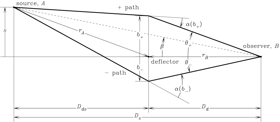
Figure 1: The geometry of either a double slit interference experiment or a two-image gravitational lens. The bold lines are the two neutrino paths, $+$ and $-$, between the source, $A$, and the observer, $B$, and the geometry is defined both in terms of physical variables ($r_{A}$, $r_{B}$, $b_{\pm}$ and $s$) and astronomical/lensing variables ($D_{d}$, $D_{s}$, $D_{ds}$, $\theta_{\pm}$ and $\beta$). Also included is the deflection angle, $\alpha_{\pm}(b)$, parameterised as a function of the physical impact parameter. It is implicit in this diagram that the deflector is rotationally symmetric, and that the paths are thus confined to the plane of the page defined by the source, deflector and observer.

III Neutrino Beam Splitter

By way of an illustrative introduction to this topic we consider a toy model of interference effects that can arise when there are both multiple paths from a source to a detector, à la Young’s double slit experiment, and different phase velocities for the propagating particles, à la neutrino oscillations. Of course, interference requires that our experimental apparatus be unable to distinguish between the propagating particles (just as we likewise require for interference that the apparatus is unable to identify which path any single particle has propagated down). We therefore require the propagating and detected particles to be different objects. In this context, let us consider, for the sake of definiteness and relevance, a Gedanken Experiment involving an imaginary (flat space) neutrino beam splitter in the geometry illustrated in Fig. 1. We take it that the neutrinos’ paths can be approximated as two straight-line segments along which momentum is constant in magnitude. We need only treat, therefore, one spatial dimension: $\int\mathbf{p}_{j}.\mathrm{d}\mathbf{x}=\int{p}_{j}\mathrm{d}x={p}_{j}|x|$, where $|x|$ is the total distance along the two line segments. We expect that the qualitative behavior of this device shall illustrate many of the features expected to emerge from interference of gravitationally lensed neutrinos. Note that for reasons of clarity we present only a plane wave treatment here, leaving a full wavepacket calculation for an appendix. We stress, however, that wave packet considerations – which allow, in particular, for a proper treatment of decoherence effects – are, in general, important and must certainly be considered when one is dealing with neutrinos that have propagated over long distances (see §6).

Let us write the ket associated with the neutrino flavour eigenstate $\alpha$ that has (in a loose sense) propagated from the source spacetime position $A=(x_{A},t_{A})$ to detection position $B=(x_{B},t_{B})$ as

$$|\nu_{\alpha};A,B\rangle=N\sum_{p}\sqrt{I_{p}}\sum_{j}U_{\alpha j}\\ \times\exp[-\mathrm{i}\Phi^{p}_{j}(E_{j};L^{AB}_{p},T^{AB})]|\nu_{j}\rangle,$$ (1)

where $T^{AB}\equiv t_{B}-t_{A}$, $L^{AB}_{p}$ is the distance from source position $x_{A}$ to detector position $x_{B}$ along one of a finite number of paths labeled by $p$, $\Phi^{p}_{j}(E_{j};L^{AB}_{p},T^{AB})\equiv E_{j}T^{AB}-p_{j}(E_{j})L^{AB}_{p}$, with $p_{j}(E_{j})$ denoting the momentum of mass eigenstate $j$ with energy $E_{j}$, and, finally, $U$ is a unitary matrix relating the neutrino flavor eigenstates to the neutrino mass eigenstates. We have included the $\sqrt{I_{p}}$ factor to account for the fact that, in general, we should allow for a path-dependence to the amplitude. A situation where, for paths $p$ and $q$, $I_{p}\neq I_{q}$ is the analog of a Young’s slit experiment in which the slits are not equally illuminated (thus reducing the visibility – see Eq. (92) – of the resulting interference fringes). The Schwarzschild lens scenario explored in §§4 and 5 presents a situation analogous to this: light or neutrinos propagating down the two classical paths from source to observer will not be, in general, equally magnified. Note that we choose throughout this paper – unless otherwise indicated – to work in units such that $\hbar=c=1\neq G$. The mass eigenstates are assumed to be on mass shell: $p_{j}(E_{j})\equiv(E_{j}^{2}-m_{j}^{2})^{1/2}$. The amplitude for a neutrino created as type $\alpha$ at the spacetime position $A$ to be detected as type $\beta$ at the spacetime position, $B$, of the detection event is then:

$$\langle\nu_{\beta}|\nu_{\alpha};A,B\rangle=N\sum_{p}\sqrt{I_{p}}\sum_{j}U_{\alpha j}U_{\beta j}^{*}\\ \times\exp[-\mathrm{i}\Phi^{p}_{j}(E_{j};L^{AB}_{p},T^{AB})].$$ (2)

Assuming a stationary source, we can get rid of the unwanted dependence on time by averaging over $T^{AB}$ in the above to determine a time-averaged oscillation probability analog at the detector position $x_{B}$ Beuthe (2003, 2002); Giunti (2003). This maneuver gives us that

$$|\langle\nu_{\beta}|\nu_{\alpha};x_{A},x_{B}\rangle|^{2}\propto\int\mathrm{d}T|\langle\nu_{\beta}|\nu_{\alpha};A,B\rangle|^{2}\\ \propto|N|^{2}\sum_{pq}\sqrt{I_{p}I_{q}}\sum_{jk}U_{\alpha j}U_{\beta j}^{*}U_{\beta k}U_{\alpha k}^{*}\\ \times\exp[\mathrm{i}(p_{j}(E)L^{AB}_{p}-p_{k}(E)L^{AB}_{q})],$$ (3)

where we have $E_{j}=E_{k}\equiv E$ because of the $\delta(E_{j}-E_{k})$ that arises from the integration over time.

We find, then, after a simple calculation that the oscillation probability analog becomes

$$|\langle\nu_{\beta}|\nu_{\alpha};x_{A},x_{B}\rangle|^{2}\\ \simeq\frac{1}{\sum_{rs}\sqrt{I_{r}I_{s}}}\sum_{pq}\sqrt{I_{p}I_{q}}\sum_{jk}U_{\alpha j}U_{\beta j}^{*}U_{\beta k}U_{\alpha k}^{*}\\ \times\exp\left[-\mathrm{i}\Delta\Phi_{jk}^{pq}\right],$$ (4)

where the phase difference is given by

$$\Delta\Phi_{jk}^{pq}\equiv-E(L^{AB}_{p}-L^{AB}_{q})+\left(\frac{m_{j}^{2}L^{AB}_{p}-m_{k}^{2}L^{AB}_{q}}{2E}\right).$$ (5)

Note that in Eq. (4) the normalization has been determined by requiring that $|\langle\nu_{\beta}|\nu_{\alpha};x_{A},x_{B}\rangle|^{2}\leq 1$. The presence of the $\leq$ sign (as opposed to a simple equality) comes about as the interference between states propagating down different paths can result in minima at which the total neutrino detection probability is zero, in which case the usual unity normalisation is impossible (so now $|\langle\nu_{\beta}|\nu_{\alpha};x_{A},x_{B}\rangle|^{2}$ no longer has a direct interpretation as a probability). This is qualitatively different behavior to that seen in neutrino oscillations where, given maximal mixing between $\nu_{\alpha}$ and $\nu_{\beta}$, an experiment might be conducted in a position where only neutrinos of type $\alpha$, say, are to be found or, alternatively, only of type $\beta$, but never in a position where none can be found in principle.

On the other hand the behavior explained above – involving interference minima and maxima – is obviously analogous to what one would expect in a double slit experiment or similar. In fact, we shall show below that the phenomenology of neutrino interference – when there is more than one path from source to detector – is a convolution of the two types of interference outlined above. This means that, in general, one cannot simply re-cast $|\langle\nu_{\beta}|\nu_{\alpha};x_{A},x_{B}\rangle|^{2}$ in terms of a conditional probability, separating out the overall interference pattern (with its nulls, etc.) from the conditional probability that any detected neutrino has certain properties. To understand this point, imagine setting all mixing angles to zero so that the mass eigenstates and weak eigenstates are identical. The point now is that the interference patterns for the various detected weak/mass eigenstates are still different: the phase difference (which now stems purely from path difference) is dependent on the mass of the neutrino species involved. In other words, $|\langle\nu_{\beta}|\nu_{\alpha};x_{A},x_{B}\rangle|^{2}$ will not, in general, factorise into a conditional probability multiplied by an interference envelope because the putative interference envelope is different for different mass eigenstates. As we show below, however, in the ultra-relativistic limit, the cross term (that mixes different path indices with different mass eigenstate indices) always turns out to be small with respect to the other terms. In this limit, then, factorization is a good approximation.

We now consider two particular, illustrative cases of the neutrino beamsplitter gedanken Experiment for which we calculate relevant phase differences and oscillation probability analogs.

III.1 Two Path Neutrino Beam Splitter

A particularly perspicuous example is given by the two-path example of the above equations. For this we specify a reference length, $L$, to which the two paths, of lengths $L_{+}$ and $L_{-}$, are related by

$$L_{\pm}\equiv L\pm\frac{\Delta L}{2}.$$ (6)

This means that there are four phase difference types as labeled by the path indices $p,q\in\{+,-\}$, viz:

$$i.\quad\Delta\Phi_{jk}^{++} = +\frac{\delta m^{2}_{jk}L+\Delta L/2}{2E}$$

$$ii.\quad\Delta\Phi_{jk}^{--} = +\frac{\delta m^{2}_{jk}L-\Delta L/2}{2E}$$

$$iii.\quad\Delta\Phi_{jk}^{+-} = -E\left(1-\frac{m_{j}^{2}+m_{k}^{2}}{4E^{2}}\right)\Delta L+\frac{\delta m^{2}_{jk}L}{2E}$$

$$iv.\quad\Delta\Phi_{jk}^{-+} = +E\left(1-\frac{m_{j}^{2}+m_{k}^{2}}{4E^{2}}\right)\Delta L+\frac{\delta m^{2}_{jk}L}{2E}.$$

In this case, then, Eq. (4) becomes

$$|\langle\nu_{\beta}|\nu_{\alpha};x_{A},x_{B}\rangle|^{2}\\ \simeq\frac{1}{I_{+}+I_{-}+2\sqrt{I_{+}I_{-}}}\\ \times\sum_{jk}U_{\alpha j}U_{\beta j}^{*}U_{\beta k}U_{\alpha k}^{*}\exp\left(-\mathrm{i}\frac{\delta m^{2}_{jk}L}{2E}\right)\\ \times\Biggl{\{}I_{+}\exp\left(+\mathrm{i}\frac{\delta m^{2}_{jk}\Delta L}{4E}\right)+I_{-}\exp\left(-\mathrm{i}\frac{\delta m^{2}_{jk}\Delta L}{4E}\right)\\ +2\sqrt{I_{+}I_{-}}\cos\left[E\left(1-\frac{m_{j}^{2}+m_{k}^{2}}{4E^{2}}\right)\right]\Biggr{\}}\,.\\$$ (8)

This is an interesting result. It shows that the interference factorises into a conventional, flat space oscillation term and an interference ‘envelope’ in curly brackets (as might be expected from a Young’s slit type experiment). If we now further particularize to the case where $I_{+}=I_{-}$, this envelope term becomes

$$\cos\left(\frac{\delta m^{2}_{jk}\Delta L}{4E}\right)+\cos\left[E\left(\!1-\frac{m_{j}^{2}+m_{k}^{2}}{4E^{2}}\right)\right]$$

$$=2\cos\!\left[E\!\left(\!1-\frac{m_{j}^{2}}{2E^{2}}\right)\!\frac{\Delta L}{2}\right]\cos\!\left[E\!\left(\!1-\frac{m_{k}^{2}}{2E^{2}}\right)\!\frac{\Delta L}{2}\right],$$

(9)

which obviously reduces to the expected photon interference term $\propto\cos^{2}$ in the massless limit. Later (in §V) we shall see that this sort of factorization property also arises, under a different set of assumptions, with gravitational lensing of astrophysical neutrinos.

III.2 Double slit experiment geometry

Having considered a hypothetical neutrino plane wave beam-splitter (§III.1), it is now possible to combine the rigorous, if simplistic, results derived above with heutristic arguments to investigate a more realistic double slit neutrino interference experiment. The choice of a double slit experiment is particularly relevant not only because of its links with more familiar interference phenomena, but also because a point-mass gravitational lens admits two (significant) paths from source to observer. Thus the results obtained in this section should provide a useful guide to the qualitative behaviour of GINI in curved space time considered in §IV.

The relevant geometry is illustrated in Fig. 1, showing the two classical paths ($+$ and $-$) from source to detector, with the important introduction of a more physically motivated set of lengths than the reference length, $L$, used previously. The entire experiment is taken to be planar, with the coordinate system origin on the line defined by the two slits. (This is an arbitrary decision at present, but will coincide with the position of the deflector in §IV.) The slits are defined by their positions, $b_{+}$ and $b_{-}$ (which will correspond to image positions in §IV.5); the source position is given by both its radial coordinate, $r_{A}$, and its perpendicular offset, $s$; the observer position is defined by its radial coordinate, $r_{B}$, alone. There are several other plausible ways in which this geometry could be defined, but all derived results become equivalent under the assumption that $|b_{\pm}|\ll r_{\{A,B\}}$, as applied throughout. Note also that the observer and source are interchangeable.

As discussed in §III, all flat-space interference phenomena can be treated in terms of path lengths. The lengths of the two paths illustrated in Fig. 1 are

$$L_{\pm} = \left(r_{B}^{2}+b_{\pm}^{2}\right)^{1/2}+\left[r_{A}^{2}-s^{2}+(b_{\pm}-s)^{2}\right]^{1/2}$$

$$\simeq (r_{A}+r_{B})\left[1+\frac{1}{2r_{A}r_{B}}\left(b_{\pm}^{2}-\frac{2r_{B}}{r_{A}+r_{B}}sb_{\pm}\right)\right],$$

where, in most cases, $b_{-}$ and $b_{+}$ are of opposite sign, and the second line explicitly utilises the fact that $|b_{\pm}|\ll r_{\{A,B\}}$. The path difference is thus

$$\Delta L_{+-} = L_{+}-L_{-}$$

$$\simeq \frac{r_{A}+r_{B}}{2r_{A}r_{B}}\left[b_{+}^{2}-b_{-}^{2}-\frac{2r_{B}}{r_{A}+r_{B}}s\left(b_{+}-b_{-}\right)\right]$$

and the average path length is

$$L \simeq (r_{A}+r_{B})$$

$$\left\{1+\frac{1}{4r_{A}r_{B}}\left[b_{+}^{2}+b_{-}^{2}-\frac{2r_{B}}{r_{A}+r_{B}}s(b_{+}+b_{-})\right]\right\}.$$

III.3 Schwarzschild slit geometry

In a laboratory-based double slit experiment the two slit positions can be chosen arbitrarily, but in the case of gravitational lensing the impact parameters of the beams are determined by a combination deflector and source parameters (§IV). Given the Schwarzschild metric around a point-mass (§IV.5), the assumption of small deflection angles implies that the source position and impact parameters are related by [cf. Eq. (75)]

$$b_{+}^{2}-b_{-}^{2}=\Delta b_{+-}^{2}\simeq\frac{r_{B}}{r_{A}+r_{B}}s\left(b_{+}-b_{-}\right).$$ (13)

Applying this result in the more general context of the double slit experiment, Eq. (13) can be rewritten as

$$\Delta L_{+-}=L_{+}-L_{-}\simeq-\frac{r_{A}+r_{B}}{2r_{A}r_{B}}\left(b_{+}^{2}-b_{-}^{2}\right).$$ (14)

Similarly, the mass-length expression that appears in, e.g., Eq. (5) can be simplified to

$$m_{j}^{2}L_{+}-m_{k}^{2}L_{-} \simeq (r_{A}+r_{B})$$

$$\mbox{}\times\left[\delta m^{2}_{jk}-\frac{1}{2r_{A}r_{B}}(m_{j}^{2}b_{+}^{2}-m_{k}^{2}b_{-}^{2})\right].$$

Substituting these expressions in Eq. (5) then gives the phase difference between mass eigenstates $j$ and $k$ travelling down paths $+$ and $-$ as

$$\Delta\Phi_{jk}^{+-}\simeq+E(r_{A}+r_{B})\frac{\Delta b_{+-}^{2}}{2r_{A}r_{B}}+\frac{\delta m^{2}_{jk}}{2E}(r_{A}+r_{B})\\ -\frac{r_{A}+r_{B}}{2E}\frac{(m_{j}^{2}b_{+}^{2}-m_{k}^{2}b_{-}^{2})}{2r_{A}r_{B}}.$$ (16)

This expression includes contributions from both different phase velocities and different path lengths, and can be understood further by considering the special cases in which (1) different mass neutrinos travel down the same path or (2) the same mass eigenstate travels down different paths.

1. From Eq. (5) for the general case of the phase difference between the same mass eigenstate propagating along different paths we find

   $$\Delta\Phi_{jj}^{pq} \equiv -\left[E-\frac{m_{j}^{2}}{2E}\right](L_{p}-L_{q})$$

   So that if we further particularize, as above, to paths passing through slits at $b_{+}$ and $b_{-}$ we find

   $$\Delta\Phi_{jj}^{+-} \simeq \left[E-\frac{m_{j}^{2}}{2E}\right]\frac{(r_{a}+r_{b})\Delta b_{+-}^{2}}{2r_{a}r_{b}}.$$

   Notice in the above the similarity to the phase difference for an ordinary Young’s double slit type experiment using photons, namely,

   $$\Delta\Phi^{pq}_{\gamma} = -\bar{E}v(L_{p}-L_{q})$$ (19)

   $$= -\left(\bar{E}-\frac{m^{2}}{2\bar{E}}\right)(L_{p}-L_{q}),$$

   where $v$ is the (phase) velocity of the interfering particle (which we assume to be relativistic). We shall see below that the analog of this phase – essentially proportional to energy $\times$ path difference – has been missed in the existing literature on neutrino oscillations in curved space. This has led to an incomplete result suggesting that the phase difference vanishes in the massless limit even when there is more than one path from source to detector.

2. Again for the general case, for the phase difference between different mass eigenstates propagating along the same path (i.e., the analog of the usual phase difference encountered in neutrino oscillation experiments), we find from Eq. (5)

   $$\Delta\Phi_{jk}^{xx} \equiv +\left(\frac{\delta m_{jk}^{2}L_{x}}{2E}\right)$$ (20)

   $$\simeq \frac{\delta m_{jk}^{2}}{2E}(L_{a}+L_{b})\left(1+\frac{b_{x}^{2}}{2L_{a}L_{b}}\right),$$

   where $x\in\{p,q\}$.

It is worth keeping the above expressions in mind when considering the results for the neutrino phase difference in curved spacetime presented in §IV.5. As will be seen, the results obtained in this more complex physical situation are analogous to those derived above, e.g., compare Eq. (1) with Eq. (58) and Eq. (20) with Eq. (59).

IV The Phase of a Neutrino Mass Eigenstate in Curved Spacetime

A neutrino beam splitter is in the realm of fantasy – except for the interesting case of gravitational lensing of neutrinos: a gravitational field can bring to a focus diverging neutrino beams, and therefore provide for multiple (classical) paths from a source to a detector. In the remainder of this paper we explore whether any interesting, quantum mechanical interference effects can arise in this sort of situation.

We shall be concerned below, therefore, with deriving an expression for the neutrino oscillation phase in curved spacetime, in particular a Schwarzschild metric (this providing the simplest case in which gravitational lensing is possible). Here we shall follow the development laid out in Fornengo et al. (1997) and Cardall and Fuller (1997) but, importantly, we shall also employ the prescription set out in §III that allows for the removal of time from consideration in the oscillation ‘probability’ by integration over $T\equiv t_{B}-t_{A}$ where $A=(\bm{r}_{A},t_{A})$ and $B=(\bm{r}_{B},t_{B})$ are the emission and detection events respectively (Beuthe, 2003) . Note that we are assuming the semi-classical limit in which gravity is not quantized and its effects can be described completely by a non-flat metric, $g_{\mu\nu}\neq\eta_{\mu\nu}$.

The procedure we follow is to start with the generalization of the equation for a mass eigenstate’s phase  in flat spacetime to curved spacetime first arrived at by Stodolsky(Stodolsky, 1979):

$$\Phi_{k}(B,A)\qquad=\qquad\int_{A}^{B}p_{\mu}^{(k)}\mathrm{d}x^{\mu},$$ (21)

where

$$p_{\mu}^{(k)}\qquad=\qquad m_{k}g_{\mu\nu}\frac{\mathrm{d}x^{\nu}}{ds},$$ (22)

is the canonically conjugate momentum to the coordinate $x^{\mu}$. Actually, as pointed out by Alsing et al. in Ref. Alsing et al. (2001), Stodolsky’s expression for the phase is missing, in general, small correction terms that arise from quantum mechanical modifications to the classical action. These vary according to the spin of the particle under consideration. Completely fortuitously, the would-be correction terms are identically zero in the case of spin half particles in a static metric (whereas for particles with, e.g., spin zero or one they are non-zero) so the Stodolsky expression happens to be exact for the Schwarzschild metric and many other cases of interest. Note in passing that this restriction to a static metric means that this technology cannot – as it stands – treat, e.g., particle phases in a cosmological context.

We now introduce the metric of the Schwarzschild spacetime. This may be written in radial co-ordinates, $x^{\mu}=(t,r,\vartheta,\varphi)$, as

$$ds^{2}\ =\ B(r)dt^{2}-B(r)^{-1}dr^{2}-r^{2}d\vartheta^{2}-r^{2}\sin^{2}\vartheta d\varphi^{2},$$ (23)

where

$$B(r)\ \equiv\ \left(1-\frac{2GM}{r}\right),$$ (24)

and $G$ is the Newtonian constant and $M$ is the mass of the source of the gravitational field, i.e., the lensing mass. Given the isotropy of the gravitational field the motion of the neutrino mass eigenstate will be confined to a plane which we take to be the equatorial one, $\vartheta=\pi/2$ and $d\vartheta=0$.

The relevant components of the canonical momentum, Eq. (22), are, then (Fornengo et al., 1997):

$$p^{(k)}_{t}=m_{k}B(r)\frac{dt}{ds},$$ (25)

$$p^{(k)}_{r}=-m_{k}B^{-1}(r)\frac{dr}{ds},$$ (26)

and

$$p^{(k)}_{\varphi}=-m_{k}r^{2}\frac{d\varphi}{ds}.$$ (27)

These are all inter-related through the mass-shell condition (Fornengo et al., 1997):

$$m^{2}_{k} = g^{\mu\nu}p_{\mu}^{(k)}p_{\nu}^{(k)}$$

$$= \frac{1}{B(r)}(p_{t}^{(k)})^{2}-B(r)(p_{r}^{(k)})^{2}-\frac{(p_{\varphi}^{(k)})^{2}}{r^{2}}.$$

Given that the components of the metric are independent of the coordinates $t$ and $\varphi$, the momenta associated with these quantities, $p^{(k)}_{t}$ and $p^{(k)}_{\varphi}$ shall be conserved along the classical geodesic traced out by $\nu_{k}$. We define these constants of motion as $E_{k}\equiv p^{(k)}_{t}$ and $J_{k}\equiv-p^{(k)}_{\varphi}$. These two are, respectively, the energy and angular momentum seen by an observer at $r\to\infty$ for the $k$th mass eigenstate (Fornengo et al., 1997). They are not identical with the energy and angular momentum that would be measured for $\nu_{k}$ at some definite, finite position $r$. In general, however, one may relate these quantities using the transformation law that relates a local reference frame $\{x^{\hat{\alpha}}\}=\{\hat{t},\hat{r},\hat{\vartheta},\hat{\varphi}\}$ to the frame $\{x^{\mu}\}=\{t,r,\vartheta,\varphi\}$ (Misner et al., 1973):

$$x^{\hat{\alpha}}=L^{\hat{\alpha}}_{\ \mu}x^{\mu},\qquad\qquad g_{\mu\nu}=L^{\hat{\alpha}}_{\ \mu}L^{\hat{\beta}}_{\ \nu}\eta_{\hat{\alpha}\hat{\beta}},$$ (29)

where the $L^{\hat{\alpha}}_{\ \mu}$’s are the coefficients of the transformation between the two bases:

$$L^{\hat{t}}_{\ t}=\sqrt{|g_{tt}|},\qquad L^{\hat{r}}_{\ r}=\sqrt{|g_{rr}|},\\ L^{\hat{t}}_{\ \vartheta}=\sqrt{|g_{\vartheta\vartheta}|},\qquad L^{\hat{\varphi}}_{\ \varphi}=\sqrt{|g_{\varphi\varphi}|}.$$ (30)

So we have, in particular, that the local energy is given by (Cardall and Fuller, 1997):

$$E_{k}^{(loc)}(r)=|g_{tt}|^{-1/2}E_{k}=B(r)^{-1/2}E_{k}.$$ (31)

IV.1 Calculating the Phase Difference

Given the above definitions, we now have that:

$$\Phi_{j}^{p}(B,A)\qquad =\qquad\int_{A}^{B}p_{\mu}^{(j)}\mathrm{d}x^{\mu}_{p}$$

$$=\int_{A}^{B}[E_{j}dt-p_{j}(r)\mathrm{d}r_{p}-J_{j}d\varphi_{p}],$$

where we have implicitly defined $p_{j}(r)\equiv-p_{r}^{(j)}$. Note that we have explicitly introduced the path index $p$ which allows for the possibility of multiple paths from source to detector. Again, however, the integration over $t$ is independent of the path as the endpoints of this integration are defined by the emission event and detection events. In fact, as discussed above, $E_{j}$ is conserved over classical paths, so that if mass eigenstate $j$ is assumed to travel down such a path, we can calculate the phase it accumulated after leaving the source to be

$$\Phi_{j}^{p}(B,A) =\int_{t_{A}}^{t_{B}}E_{j}dt-\int_{r_{A}}^{r_{B}}\left[p_{j}(r)+J_{j}\left(\frac{d\varphi}{dr}\right)_{j}^{p}\right]\mathrm{d}r_{p}$$ (33)

$$=E_{j}(t_{B}-t_{A})$$

$$\qquad-\int_{r_{A}}^{r_{B}}\left[p_{j}(r)+J_{j}\left(\frac{d\varphi}{dr}\right)_{j}^{p}\right]\mathrm{d}r_{p}.$$

Of course, the quantity that governs the oscillation phenomenology is the phase difference $\Delta\Phi_{kj}^{pq}$ where, generically, interference can be between different mass eigenstates and/or different paths (cf. discussion in §III). As things stand this quantity would be parameterized in terms of both $t$ and $r$:

$$\Delta\Phi_{jk}^{pq}(r_{B},t_{B},r_{A},t_{A})=(E_{j}-E_{k})(t_{B}-t_{A})\\ -\Biggl{\{}\int_{r_{A}}^{r_{B}}\left[p_{j}(r)+J_{j}\left(\frac{d\varphi}{dr}\right)_{j}^{p}\right]\mathrm{d}r_{p}\\ -\int_{r_{A}}^{r_{B}}\Biggl{[}p_{k}(r)+J_{k}\left(\frac{d\varphi}{dr}\right)_{k}^{q}\Biggr{]}\mathrm{d}r_{q}\Biggr{\}}.$$ (34)

We therefore follow the prescription set out in Beuthe (2003) to rid ourselves of the unwanted time parameter: we assume a stationary source and integrate the interference term, $\exp\left[-\mathrm{i}\Delta\Phi_{kj}^{pq}\right]$, over the unknown emission time $t_{A}$ (or, equivalently, the transmission time $T\equiv t_{B}-t_{A}$). This results in a very useful $\delta(E_{j}-E_{k})$.

Note here that though the energies of different mass eigenstates are different (Giunti, 2001) – so that the $\delta\left(E_{k}-E_{j}\right)$ arising from the time integration would seem to imply no interference – in fact, in a correct treatment, massive neutrinos are described by wave packets, not plane waves as here. This means that, though the average energies of different mass eigenstate wave packets are, in general, different, each massive neutrino wave packet has an energy spread and the detection process can pick up the same energy component for different massive neutrinos (see Refs. Beuthe (2003); Giunti (2002b)). If the energy spread of the wave packets is small there is a suppression factor that, formally, can only be calculated only with a wave packet treatment (cf. §III), but, can also be assessed at the heuristic level (cf. §VI).

Let us see how all the above works in practice.

IV.2 Radial Propagation

We consider first the simple case of radial propagation, in which case there is a single classical path from source to detector. Along this path, the angular momentum vanishes and we have:

$$\Delta\Phi_{jk}(r_{B},t_{B},r_{A},t_{A})=(E_{j}-E_{k})(t_{B}-t_{A})$$

$$-\int_{r_{A}}^{r_{B}}[p_{j}(r)-p_{k}(r)]\mathrm{d}r$$ (35)

We can determine $p_{j}(r)-p_{k}(r)$ from the mass-shell relation, Eq. (IV) (Fornengo et al., 1997):

$$p_{k}(r)=\pm\frac{1}{B(r)}\sqrt{E_{k}^{2}-B(r)m_{k}^{2}},$$ (36)

where the $+$ sign refers to neutrinos propagating outwards from the gravitational well and the $-$ sign to neutrinos propagating inwards. We can further simplify this relation by employing the binomial expansion which, as in the flat space case, holds for relativistic particles:

$$\sqrt{E_{k}^{2}-B(r)m_{k}^{2}} \simeq E_{k}-B(r)\frac{m_{k}^{2}}{2E_{k}},$$ (37)

where $E_{0}$ is the energy at infinity for a neutrino mass eigenstate in the massless limit (see Fornengo et al. (1997) for a detailed account of the region of applicability of Eq. (37)). We therefore have that

$$p_{j}(r)-p_{k}(r)\simeq\pm\frac{1}{B(r)}(E_{j}-E_{k})\mp\left(\frac{m^{2}_{j}}{2E_{j}}-\frac{m^{2}_{k}}{2E_{k}}\right).$$ (38)

The phase difference then becomes

$$\Delta\Phi_{jk}(r_{B},t_{B},r_{A},t_{A})\\ \simeq(E_{j}-E_{k})\left[(t_{B}-t_{A})\mp\int_{r_{A}}^{r_{B}}\frac{\mathrm{d}r}{B(r)}\right]\\ +\left(\frac{m^{2}_{j}}{2E_{j}}-\frac{m^{2}_{k}}{2E_{k}}\right)|r_{B}-r_{A}|.$$ (39)

Given the oscillation ‘probability’ shall be, following our previously-establsihed procedure (cf. §III), integrated over $T\equiv t_{B}-t_{A}$, the relevant phase difference can be seen to be

$$\Delta\Phi_{jk}(r_{B},r_{A}) \simeq \frac{\delta m_{jk}^{2}}{2E_{\nu}}\left|r_{B}-r_{A}\right|$$ (40)

$$\simeq \frac{\delta m_{jk}^{2}}{2E_{0}}\left|r_{B}-r_{A}\right|\,.$$

where $E_{\nu}=E_{j}=E_{k}$ and $E_{0}$ is the energy at infinity for a massless particle and, as in flat space, the following relation holds (Fornengo et al., 1997):

$$E_{k}\simeq E_{0}+{\cal O}\left(\frac{m_{k}^{2}}{2E_{0}}\right).$$ (41)

To digress a little, note that the result presented in Eq. (40), arrived at previously (Bhattacharya et al., 1996; Fornengo et al., 1997; Cardall and Fuller, 1997; Bhattacharya et al., 1999), must be interpreted with some care: in Eq. (40) one must keep in mind that the radial distance $\left|r_{B}-r_{A}\right|$ is a coordinate distance, and not the proper distance the various mass eigenstates experience (except in the flat space case to which Eq. (40) clearly reduces in the limit of a vanishing lensing mass) and that $E_{0}$ does not represent a locally-detected energy. Following Fornengo et al. (1997), however, we can convert the phase difference so that it appears in terms of these parameters. The proper distance is given by (cf. Eq. (30)):

$$L_{\mathrm{prop}} \equiv\int^{r_{B}}_{r_{A}}\sqrt{g_{rr}}\mathrm{d}r$$ (43)

$$\simeq r_{B}-r_{A}+GM\ln\frac{r_{B}}{r_{A}},$$

where in the second line we have assumed the weak field limit holds. This demonstrates that, in a gravitational field, the length relevant to the calculation of phases, $|r_{B}-r_{A}|$, is actually shorter than the distances experienced by the propagating particles, $L_{\mathrm{prop}}$. Substituting Eqs. (31) and (43) into (40) we determine that (cf. (Fornengo et al., 1997)):

$$\Delta\Phi_{jk}(r_{B},r_{A}) \simeq \left(\frac{\Delta m^{2}_{jk}L_{\mathrm{prop}}}{2E_{0}^{(loc)}(r_{B})}\right)$$

$$\times\left[1-GM\left(\frac{1}{L_{\mathrm{prop}}}\,\ln\frac{r_{B}}{r_{A}}-\frac{1}{r_{B}}\right)\right]\;.$$

IV.3 Non-Radial Propagation

We turn now to the more interesting case presented by non-radial propagation. Here there will be, generically, more than one path for the mass eigenstates to take from source to detector and we have the possibility, therefore, of interference between particles on these different paths.

The phase difference we must calculate is given by Eq. (34). To proceed with this calculation we must determine a value for

$$p_{j}(r)+J_{j}\left(\frac{d\varphi}{dr}\right)_{j}^{p}.$$

Firstly recall that $J_{j}$ is constant along the classical path taken by $\nu_{j}$. Now, using the fact (see Landau and Lifshitz (1975), Eq.(101.5)) that

$$\left(\frac{\mathrm{d}\phi}{\mathrm{d}r}\right)_{j}^{p} = \pm\frac{J_{j}^{p}}{r^{2}\sqrt{E_{j}^{2}-\left(m_{j}^{2}+\frac{(J_{j}^{p})^{2}}{r^{2}}\right)B(r)}}$$

$$\simeq \pm\frac{b_{p}\left(1-\frac{m_{j}^{2}}{2E_{j}}\right)}{r^{2}\sqrt{1-\frac{B(r)}{E_{j}^{2}}\left[m_{j}^{2}+\frac{E_{j}^{2}b_{p}^{2}}{r^{2}}\left(1-\frac{m_{j}^{2}}{E_{j}^{2}}\right)\right]}},$$

and, given that from the mass-shell relation we have [see Eq. (49) of Fornengo et al. (1997)]:

$$B(r)p_{j}(r) \simeq \pm\sqrt{1-B(r)\frac{b_{p}^{2}}{r^{2}}}$$ (46)

$$\times\left[1-\frac{B(r)(1-b_{p}^{2}/r^{2})}{1-B(r)b_{p}^{2}/r^{2}}\frac{m_{j}^{2}}{2E^{2}_{j}}\right],$$

where $b_{p}$ is the impact parameter for path $p$, one may determine that:

$$p_{j}(r)+J_{j}^{p}\left(\frac{\mathrm{d}\phi}{\mathrm{d}r}\right)_{j}^{p}\simeq\pm\frac{E_{j}}{B(r)\sqrt{1-B(r)\frac{b_{p}^{2}}{r^{2}}}}\\ \mp\frac{m_{j}^{2}}{2E_{j}^{2}}\frac{1+(1-2B(r))\frac{b_{p}^{2}}{r^{2}}}{\left(1-B(r)\frac{b_{p}^{2}}{r^{2}}\right)^{\frac{3}{2}}}.$$ (47)

In the above we have also employed the fact that the angular momentum of mass eigenstate $j$ (traveling along path $p$) at infinity is given in terms of $\nu_{j}$’s energy at infinity, $E_{j}$, the impact parameter along the path being considered, $b_{p}$, and $\nu_{j}$’s velocity at infinity, $v_{j}^{(\infty)}$ (Fornengo et al., 1997):

$$J_{j}^{p} =E_{j}b_{p}v_{j}^{(\infty)}$$ (48)

$$\simeq E_{j}b_{p}\left(1-\frac{m_{j}^{2}}{2E_{j}^{2}}\right).$$

We can further evaluate Eq. 47 by replacing the path-dependent impact parameter, $b_{p}$, with the minimal radial co-ordinate for the same path, $r_{0}^{p}$. The relation between these two is found by noting that at the position of closest approach the rate of change of the co-ordinate $r$ with respect to the angle $\phi$ vanishes (Fornengo et al., 1997). For the massive case (Eq. IV.3), this implies that:

$$b_{p}^{2}\simeq\frac{1+\frac{m_{j}^{2}}{E_{j}^{2}}\frac{2GM}{r^{p}_{0}}}{B(r^{p}_{0})}\,.$$ (49)

Employing Eq. (49), taking the weak field limit, and also expanding to ${\cal O}(m_{j}^{2}/E_{j}^{2})$ we find that:

$$p_{j}(r)+J_{j}^{p}\left(\frac{\mathrm{d}\phi}{\mathrm{d}r}\right)_{j}^{p}\\ \simeq\pm E_{j}\left[\frac{r}{\sqrt{r^{2}-(r^{p}_{0})^{2}}}+GM\frac{2r-3r^{p}_{0}}{\sqrt{r^{2}-(r^{p}_{0})^{2}}(r+r^{p}_{0})}\right]\\ \mp\frac{m_{j}^{2}}{E_{j}}\left[\frac{r}{\sqrt{r^{2}-(r^{p}_{0})^{2}}}-GM\frac{r^{p}_{0}}{\sqrt{r^{2}-(r^{p}_{0})^{2}}(r+r^{p}_{0})}\right]\\$$ (50)

With this result in hand, we can complete the calculation of Eq. (33), the phase accumulated by mass eigenstate in non-radial propagation from spacetime position $A=(r_{A},t_{A})$ to $B=(r_{B},t_{B})$, where either $r_{A}$ or $r_{B}$ is the minimal radial co-ordinate encountered over the journey (i.e. the path is either non-radially inwards or outwards but not both). After an elementary integration we find that

$$\Phi_{j}^{p}(B,A)\simeq E_{j}(t_{B}-t_{A})\\ \mp E_{j}\left[\sqrt{r_{B}^{2}-(r^{p}_{0})^{2}}-\sqrt{r_{A}^{2}-(r^{p}_{0})^{2}}\right.\\ +2GM\ln\left(\frac{r_{B}+\sqrt{r_{B}^{2}-(r^{p}_{0})^{2}}}{r_{A}+\sqrt{r_{A}^{2}-(r^{p}_{0})^{2}}}\right)\\ \left.+GM\left(\sqrt{\frac{r_{B}-r^{p}_{0}}{r_{B}+r^{p}_{0}}}-\sqrt{\frac{r_{A}-r^{p}_{0}}{r_{A}+r^{p}_{0}}}\right)\right]\\ \pm\frac{m_{j}^{2}}{2E_{j}}\left[\sqrt{r_{B}^{2}-(r^{p}_{0})^{2}}-\sqrt{r_{A}^{2}-(r^{p}_{0})^{2}}\right.\\ \left.\qquad\qquad-GM\left(\sqrt{\frac{r_{B}-r^{p}_{0}}{r_{B}+r^{p}_{0}}}-\sqrt{\frac{r_{A}-r^{p}_{0}}{r_{A}+r^{p}_{0}}}\right)\right],\\$$ (51)

where the upper signs pertain if $dr$ is positive (outward propagation) and the lower if $dr$ is negative.

IV.4 Neutrino Lensing

Finally let us consider the case of gravitational lensing of neutrinos. In this case the neutrinos propagate non-radially along classical paths, labelled by index $p$, from radial position $r_{A}$, inwards to a path-dependent minimal radial co-ordinate $r_{0}^{p}$, and outwards again to a detector situated at radial co-ordinate $r_{B}$. As presaged above, in this situation there will be (at least potentially) interference not only between different mass eigenstates propagating down the same classical path, but also between mass eigenstates propagating down different paths ($p$ and $q$, say). Taking into account the sign of the momentum along these two legs, we find, following the developments above, that the relevant phase is given by

$$\Phi_{j}^{p}(B,A)\\ \simeq E_{j}(t_{B}-t_{A})\\ -E_{j}\left[\sqrt{r_{A}^{2}-(r^{p}_{0})^{2}}+2GM\ln\left(\frac{r_{A}+\sqrt{r_{A}^{2}-(r^{p}_{0})^{2}}}{r^{p}_{0}}\right)\right.\\ \left.+GM\left(\sqrt{\frac{r_{A}-r^{p}_{0}}{r_{A}+r^{p}_{0}}}\right)+(r_{A}\to r_{B})\right]\\ +\frac{m_{j}^{2}}{2E_{j}}\Biggl{[}\sqrt{r_{A}^{2}-(r^{p}_{0})^{2}}\\ -GM\left(\sqrt{\frac{r_{A}-r^{p}_{0}}{r_{A}+r^{p}_{0}}}\right)+(r_{A}\to r_{B})\Biggr{]},\\$$ (52)

where $(r_{A}\to r_{B})$ mean add another term of the same form but with $r_{A}$ replaced with $r_{B}$.

Before proceeding any further with the calculation it behooves us here to establish the plausibility of Eq. (52) by showing its relation to results known from some simpler cases. In the $M\to 0$ limit this equation becomes

$$\Phi_{j}^{p}(B,A) \simeq E_{j}(t_{B}-t_{A})-E_{j}\left(1-\frac{m_{j}^{2}}{2E_{j}^{2}}\right)$$

$$\qquad\times\left[\sqrt{r_{A}^{2}-(r^{p}_{0})^{2}}+\sqrt{r_{B}^{2}-(r^{p}_{0})^{2}}\right].$$

Now refer back to Fig. 1, and take the coordinate origin on the diagram to denote the position of a lensing point mass. In the massless case, the two classical paths reduce to the single ‘undeflected’ path denoted by the dashed line in the diagram. Denote the minimal radial coordinate along this path by $r_{0}$ (which intersects the dashed line at right angles). Clearly, then, the geometrical length of the path from source to detector is $\sqrt{r_{A}^{2}-r_{0}^{2}}+\sqrt{r_{B}^{2}-r_{0}^{2}}$. Now, given we know that in flat space the phase of mass eigenstate $k$ is given by Eq. (21) with Minkowski metric, viz:

$$\Phi_{j}\qquad=\qquad E_{j}(t_{B}-t_{A})-\bm{p}_{j}.(\bm{x}_{B}-\bm{x}_{A}).$$ (54)

then, for the $M\to 0$ case illustrated in Fig. 1 this becomes

$$\Phi_{j} \simeq E_{j}(t_{B}-t_{A})-E_{j}\left(1-\frac{m_{j}^{2}}{2E_{j}^{2}}\right)$$

$$\qquad\qquad\times\left(\sqrt{r_{A}^{2}-r_{0}^{2}}+\sqrt{r_{B}^{2}-r_{0}^{2}}\right).$$

With Eq. (IV.4) we have, then independently established the plausibility of Eq. (IV.4), once one takes into account the fact that, in the massless lens case, all classical paths converge on the same undeflected path (as mentioned above) so that in this limit $r_{0}^{p}=r_{0}^{q}\equiv r_{0}$ $\forall p,q$.

The other limit of interest is to take $m_{j}\to 0$ in Eq. (52). In doing this – and then setting the temporal and spatial contributions to the phase equal as appropriate for a null geodesic – we find that we have re-derived the Shapiro time delay [see, e.g., Eq. (8.7.4) of Ref. (Weinberg, 1972)].

Continuing with our main calculation, we can re-write Eq. (52) in terms of $b_{p}$ by inverting Eq. (49). If we also expand to ${\cal O}(b_{p}^{2}/r^{2}_{B\leftrightarrow A})$, we find that

$$\Phi_{j}^{p}(B,A)\\ \simeq E_{j}(t_{B}-t_{A})\\ \qquad-E_{j}(r_{A}+r_{B})\\ \times\left\{1-\frac{b_{p}^{2}}{2r_{A}r_{B}}+\frac{2GM}{r_{A}+r_{B}}\left[1+\ln\left(\frac{4r_{A}r_{B}}{b_{p}^{2}}\right)\right]\right\}\\ +\frac{m_{j}^{2}}{2E_{j}}(r_{A}+r_{B})\left(1-\frac{b_{p}^{2}}{2r_{A}r_{B}}-\frac{2GM}{r_{A}+r_{B}}\right).\\$$ (56)

We can now find the phase difference, which allows for interference between different paths and/or different mass eigenstates, by the usual integration over $T$ (so that we have $E_{\nu}=E_{j}=E_{k}$):

$$\Delta\Phi_{jk}^{pq}(r_{B},r_{A})\\ \simeq+E_{\nu}(r_{A}+r_{B})\left(\frac{\Delta b_{pq}^{2}}{2r_{A}r_{B}}+\frac{4GM}{r_{A}+r_{B}}\ln\left|\frac{b_{p}}{b_{q}}\right|\right)\\ +\frac{\delta m_{jk}^{2}}{2E_{\nu}}(r_{A}+r_{B})\left(1-\frac{2GM}{r_{A}+r_{B}}\right)\\ -\frac{r_{A}+r_{B}}{2E_{\nu}}\left(\frac{m_{j}^{2}b_{p}^{2}-m_{k}^{2}b_{q}^{2}}{2r_{A}r_{B}}\right),\\$$ (57)

where $\Delta b^{2}_{pq}\equiv b^{2}_{p}-b^{2}_{q}$ and, in our notation, $\Delta\Phi_{jk}^{pq}(r_{B})$ denotes the phase difference between mass eigenstate $j$ traveling down path $p$ and mass eigenstate $k$ traveling down path $q$ . Eq. (57) is one of the major results of this paper. Note that the presence of the $\propto E_{\nu}$ term in this equation – missed in Ref. (Fornengo et al., 1997) – ensures that the phase difference behaves properly in the massless limit (i.e., does not vanish). In passing, also note that the above equation satisfies the discrete symmetry of swapping $B$ and $A$, as it should: the same result must be obtained for the phase difference (in a static spacetime) if we swap the positions of source and observer.

Also recall that, excluding the case of perfect alignment of source, lens, and observer, there are only two possible classical paths from source to observer for the Schwarzschild case. These we label by $+$ (this path having an impact parameter somewhat greater than the impact parameter for an undeflected ray) and $-$ (this path having an impact parameter on the ‘opposite’ side of the lens to the undeflected ray). We require, therefore, that $p,q\in\{+,-\}$ and in the particular case that we are considering interference between the same mass eigenstates propagating down different paths Eq. (57) becomes

$$\Delta\Phi_{jj}^{+-}(r_{B},r_{A})\\ \simeq+E_{\nu}(r_{A}+r_{B})\left(\frac{\Delta b_{+-}^{2}}{2r_{A}r_{B}}+\frac{4GM}{r_{A}+r_{B}}\ln\left|\frac{b_{+}}{b_{-}}\right|\right)\\ -\frac{m_{j}^{2}}{2E_{\nu}}(r_{A}+r_{B})\frac{\Delta b_{+-}^{2}}{2r_{A}r_{B}}.\\$$ (58)

Alternatively, in the case of different mass eigenstates traveling down the same path (i.e., ‘ordinary’ neutrino oscillations, but in curved space), Eq. (57) becomes

$$\Delta\Phi_{jk}^{pp}(r_{B},r_{A})\simeq\frac{\delta m_{jk}^{2}}{2E_{\nu}}(r_{A}+r_{B})\\ \times\left(1-\frac{b_{p}^{2}}{2r_{A}r_{B}}-\frac{2GM}{r_{A}+r_{B}}\right).$$ (59)

Note that Eqs. (57), (58), and (59) give us that

$$\Delta\Phi_{jk}^{pq}(r_{B},r_{A})=\Delta\Phi_{jj}^{pq}(r_{B},r_{A})+\Delta\Phi_{jk}^{pp}(r_{B},r_{A})\\ +{\cal O}\left[\frac{\delta m_{jk}^{2}}{2E_{\nu}}(r_{A}+r_{B})\frac{\Delta b_{pq}^{2}}{2r_{A}r_{B}}\right].$$ (60)

This correction term will be small with respect to other terms (given our assumptions of ultra-relativistic neutrinos and undeflected impact parameters small with respect to the overall distances between source-lens and lens-observer). In fact, the third term of Eq. (57) can be expected to be suppressed with respect to the first term by ${\cal O}(m^{2}/E^{2}_{\nu})$ and with respect to the second term by ${\cal O}(b^{2}/(r_{A}r_{B}))$. The consequence of this is that the phase may be written

$$\Delta\Phi^{pq}_{jk}\simeq\Delta\Phi_{jk}+\Delta\Phi^{pq},$$ (61)

satisfying what we label ‘separability’, where

$$\Delta\Phi^{pq}\equiv E_{\nu}(r_{A}+r_{B})\left(\frac{\Delta b_{pq}^{2}}{2r_{A}r_{B}}+\frac{4GM}{r_{A}+r_{B}}\ln\left|\frac{b_{p}}{b_{q}}\right|\right)$$

$$-\frac{\overline{m}^{2}}{2E_{\nu}}(r_{A}+r_{B})\frac{\Delta b_{pq}^{2}}{2r_{A}r_{B}}.$$

and

$$\Delta\Phi_{jk} \equiv \frac{\delta m_{jk}^{2}}{2E_{\nu}}(r_{A}+r_{B})\left(1-\frac{\overline{b}^{2}}{2r_{A}r_{B}}-\frac{2GM}{r_{A}+r_{B}}\right),$$

where

$$\overline{m}\equiv\frac{1}{N_{\nu}}\sum^{N_{\nu}}_{j}m_{j} \overline{b}\equiv\frac{1}{N_{\textrm{path}}}\sum^{N_{\textrm{path}}}_{j}b_{p},$$ and (64)

with $N_{\nu}$ the number of neutrino mass eigenstates and $N_{\textrm{path}}$ the number of classical paths from source to detector (two in the case of the Schwarzschild metric). What Eq. (61) says in words is that the phase difference that develops between source and detector is due to two effects that can be considered separately: (i) a phase difference – independent of which mass eigenstate is under consideration – that develops because of the different lengths of the paths involved and (ii) the phase difference that develops because the different mass eigenstates travel with different phase velocites. This situation is analogous to two runners who run along two very similar – though not identical – paths, with similar – though not identical – velocities: to first order, the difference in the finishing times between the two depends on terms proportional to the difference in lengths of the two courses, $\Delta L$, and the difference in the runners’ velocities, $\Delta v$, but not, by definition, on terms $\propto\Delta L\,\Delta v$.

IV.5 Phase Difference in Terms of Conventional Lensing Parameters

To facilitate interpretation of the above results in an astrophysical context – and, eventually, to introduce an evolving cosmological model – it is useful to re-express the phase difference in the language of standard gravitational lensing theory (despite the fact that the particles being lensed are not photons).

IV.5.1 The lens equation

The classically allowed neutrino paths in the presence of a deflector can be derived by reconsidering the geometry shown in Fig. 1. Under the assumption that $|b_{\pm}|\ll r_{\{A,B\}}$, the source offset, $s$, can be related to the impact parameter, $b$, by the lens equation:

$$s\simeq\frac{r_{B}}{r_{A}+r_{B}}b+r_{A}\,\alpha(b),$$ (65)

where $\alpha(b)$ is the deflection angle of the lens as a function of impact parameter.

It is standard practice to reexpress the lens equation in terms of angular variables. This entails replacing the source offset and impact parameters with angles (on the sky of the observer) and radial coordinates with line-of-sight distances. These conversions are summarised graphically in Fig. 1, which leads to the following replacements: $r_{A}\to({D_{ds}^{2}+s^{2}})^{1/2}\simeq D_{ds}$, where $D_{ds}$ is the distance from deflector to source; $r_{B}\to D_{d}$, where $D_{d}$ is the distance from observer to deflector; and $r_{A}+r_{B}\to D_{s}$, where $D_{s}$ is the distance from observer to source. The notation employed for the distance measures is suggestive of their being the angular diameter distances used to relate angles and lengths in an evolving cosmological model, and they fulfil an analogous role here. It is most important to note, however, that they are not true angular diameter distances and the following results are only quantitatively valid on scales sufficiently small that the expansion of the Universe can be ignored (e.g., the Milky Way or the Local Group). These results will be extended to an evolving cosmology in (Crocker and Mortlock, 2003).

The above caveats notwithstanding, the angular position (relative to the deflector) of an image with impact parameter $b$ is now simply

$$\theta\simeq\frac{b}{r_{B}}\simeq\frac{b}{D_{d}},$$ (66)

and the position of the source can be given in terms of an unobservable angular parameter $\beta$ as

$$\beta\simeq\frac{s}{r_{A}+r_{B}}\simeq\frac{s}{D_{s}}.$$ (67)

Inserting these definitions into Eq. (65), the lens equation becomes

$$\beta\simeq\theta+\frac{D_{ds}}{D_{s}}\alpha(D_{d}\theta).$$ (68)

The position(s) of the images formed by a source in a given position can then be found for a given choice of deflector model.

IV.5.2 The Schwarzschild lens

In a Schwarzshild metric, the total angular deflection of a particle of mass $m$ impinging on a point-mass $M$ with undeflected impact parameter $b$ is (see, e.g., Schneider et al. (1992)):

$$\alpha_{\rm{gen}}(b)=-\frac{4GM}{b}\frac{1}{2}\left(1+\frac{1}{v_{\infty}^{2}}\right),$$ (69)

where $v_{\infty}$ is the particle’s speed at an infinite distance from the mass and it has been assumed that $b\gg 2GM=R_{S}$, the deflector’s Schwarzschild radius. For an ultra-relativistic particle, this becomes

$$\alpha_{\rm{rel}}(b)\simeq-\frac{4GM}{b}\left(1+\frac{m^{2}}{2E^{2}}\right),$$ (70)

where $E$ is its coordinate energy (equal to the energy measured at an infinte distance from the mass).

For astrophysical neutrinos, however, $m^{2}/(2E^{2})\ll 1$ and so it is an excellent approximation to assume they travel along classical photon paths, for which

$$\alpha_{\rm{light}}(b)=-\frac{4GM}{b}.$$ (71)

Previously we have been rigorous in taking the classical paths of massive particles from source to observer but, as will be seen below, this assumption is entirely self-consistent when dealing with weak-field gravitational effects and ultra-relativistic particles. Note also that a corollary of this approximation is that the different mass eigenstates are assumed to travel down identical paths (whereas in reality the heavier eigenstates will fall marginally deeper into the deflector’s potential well).

Applying the above deflection law to Eq. (68) gives the point-mass lens equation as

$$\beta\simeq\theta-\frac{\theta_{E}^{2}}{\theta}$$ (72)

where

$$\theta_{E}=\sqrt{4GM\frac{D_{ds}}{D_{d}D_{s}}}$$ (73)

is the Einstein radius of the lens. This is the angular radius of the circular image that would be formed in the case of perfect source-deflector-observer alignment (i.e., $\beta=0$) and thus depends on distance factors as well as the lens mass. Solving the lens equation then gives the image positions as

$$\theta_{\pm}\simeq\frac{1}{2}\left(\beta\pm\sqrt{\beta^{2}+4\theta_{\rm{E}}^{2}}\right).$$ (74)

This also implies the useful Schwarzschild-specific result that

$$\theta_{+}^{2}-\theta_{-}^{2}=\Delta\theta^{2}_{+-}\simeq\beta(\theta_{+}-\theta_{-}).$$ (75)

Having found a relationship between the angular position of a neutrino source and its images, the expression for the phase difference given in Eq. (57) can be recast in a form containing only line-of-sight distances and angular variables. This yields the Schwarzschild-specific result that

$$\Delta\Phi_{jk}^{pq} \simeq E_{\nu}\,\frac{D_{d}D_{s}}{D_{ds}}\left[\frac{\Delta\theta^{2}_{pq}}{2}+\theta_{\rm{E}}^{2}\,\ln\left(\left|\frac{\theta_{p}}{\theta_{q}}\right|\right)\right]$$ (76)

$$+ \frac{\delta m_{jk}^{2}}{2E_{\nu}}D_{s}\left(1-\frac{D_{d}}{D_{ds}}\theta_{\rm{E}}^{2}\right)$$

$$- \frac{1}{2E_{\nu}}\frac{D_{d}D_{s}}{D_{ds}}\frac{m_{j}^{2}\theta_{p}^{2}-m_{k}^{2}\theta_{q}^{2}}{2}.$$

The second term in this equation is simply the phase difference that develops between mass eigenstates $j$ and $k$ traveling along the same path for distance $D_{s}$, with a small correction for the presence of the deflector. The first term encodes the path difference along the trajectories $p$ and $q$, with separate contributions from the geometrical effect ($\propto\Delta\theta_{pq}^{2}$) and the reduced coordinate velocity close to the deflector [$\propto\ln(|\theta_{p}/\theta_{q}|)$]. The final cross term is the leading order contribution from different eigenstates traveling down different paths. From the discussion in the previous section, this term will be small in general.

Given that interference effects can only ever be important when the detector cannot resolve different image positions (i.e., it cannot know down which path the neutrino has travelled), having the phase difference in terms of $\theta_{p}$ and $\theta_{q}$ is not as useful as expressing it as a function of the (angular) source position, $\beta$.

For the Schwarzschild lens the conversion from $\theta$ to $\beta$ is given in Eq. (72), and substituting this into Eq. (76) then gives (for mass eigenstate $j$ down path $+$ and mass eigenstate $k$ down path $-$)

$$\Delta\Phi_{jk}^{+-} \simeq E_{\nu}\frac{D_{d}D_{s}}{D_{ds}}\Biggl{[}\frac{\beta\sqrt{\beta^{2}+4\theta_{\rm{E}}^{2}}}{2}$$

$$\qquad\qquad\qquad+\theta_{\rm{E}}^{2}\ln\left(\left|\frac{\beta+\sqrt{\beta^{2}+4\theta_{\rm{E}}^{2}}}{\beta-\sqrt{\beta^{2}+4\theta_{\rm{E}}^{2}}}\right|\right)\Biggr{]}$$

$$+ \frac{\delta m_{jk}^{2}}{2E_{\nu}}D_{s}\left(1-\frac{D_{d}}{D_{ds}}\theta_{\rm{E}}^{2}\right)$$

$$- \frac{1}{2E_{\nu}}\frac{D_{d}D_{s}}{D_{ds}}\frac{1}{4}\Biggl{[}\delta m_{jk}^{2}(\beta^{2}+2\theta_{\rm{E}}^{2})$$

$$\qquad\qquad\qquad\qquad+(m_{j}^{2}+m_{k}^{2})\beta\sqrt{\beta^{2}+4\theta_{\rm{E}}^{2}}\Biggr{]}.$$

Thus the phase difference is expressed in terms of essntially independent astronomical variables: the line-of-sight distances between observer, deflector and source, the mass of the deflector (encoded uniquely in $\theta_{\rm{E}}$ once the distances have been chosen) and the perpendicular source offset, $\beta$.

Most of the important results obtained towards the end of §IV.4 can be recast similarly in terms of standard lensing variables, either in terms of the unobservable image positions or the source position. Assuming separability (see §IV.4), for instance, the contribution to the $\Delta\Phi$ due to path difference effects alone (Eq. IV.4) can be written as

$$\Delta\Phi^{pq} \simeq E_{\nu}\,\frac{D_{d}D_{s}}{D_{ds}}\left[\frac{\Delta\theta^{2}_{pq}}{2}+\theta_{\rm{E}}^{2}\,\ln\left(\left|\frac{\theta_{p}}{\theta_{q}}\right|\right)\right]$$ (78)

$$- \frac{\bar{m}^{2}}{2E_{\nu}}\frac{D_{d}D_{s}}{D_{ds}}\frac{\Delta\theta^{2}_{pq}}{2}$$

which for $p=+$ and $q=-$ becomes

$$\Delta\Phi^{+-} \simeq E_{\nu}\frac{D_{d}D_{s}}{D_{ds}}\Biggl{[}\frac{\beta\sqrt{\beta^{2}+4\theta_{\rm{E}}^{2}}}{2}$$ (79)

$$\qquad\qquad\qquad+\theta_{\rm{E}}^{2}\,\ln\left(\left|\frac{\beta+\sqrt{\beta^{2}+4\theta_{\rm{E}}^{2}}}{\beta-\sqrt{\beta^{2}+4\theta_{\rm{E}}^{2}}}\right|\right)\Biggr{]}$$

$$-\frac{\bar{m}^{2}}{2E_{\nu}}\frac{D_{d}D_{s}}{D_{ds}}\frac{\beta\sqrt{\beta^{2}+4\theta_{\rm{E}}^{2}}}{2}.$$

Similarly, the contribution due solely to the different phase velocities of two mass eigenstates traveling down the same path (Eq. IV.4) can be expressed as

$$\Delta\Phi_{jk}\simeq\frac{\delta m_{jk}^{2}}{2E_{\nu}}D_{s}\left[1-\frac{\theta_{\rm{E}}^{2}}{8}\left(\beta^{2}+4\theta_{\rm{E}}^{2}\right)\right].$$ (80)

V The Oscillation ‘Probability’

With the above results, we can now calculate the analog, in curved space, of the flat-space neutrino oscillation probability:

$$|\langle\nu_{\beta}|\nu_{\alpha},D_{s}\rangle|^{2}\propto\int\mathrm{d}T|\langle\nu_{\beta}|\nu_{\alpha};A,B)\rangle|^{2}$$ (81)

so that we can write

$$|\langle\nu_{\beta}|\nu_{\alpha},D_{s}\rangle|^{2}\\ =|N|^{2}\sum_{pq}\sqrt{I_{p}I_{q}}\sum_{jk}U_{\alpha j}U_{\beta j}^{*}U_{\beta k}U_{\alpha k}^{*}\\ \times\exp\left[-\mathrm{i}\Delta\Phi_{jk}^{pq}(D_{s})\right],$$ (82)

where $I_{p}$ and $I_{q}$ account for the fact that different paths may be differentially magnified by a lens. We remind the reader that $|\langle\nu_{\beta}|\nu_{\alpha},D_{s}\rangle|^{2}$ is no longer strictly a probability – see §III.

In the case that the ‘separability’ defined by Eq. (61) is satisfied, if, for the moment, we are interested only in determining the (energy) spacing of the interference maxima and minima, we need only consider a plane-wave-like calculation (and can therefore set to one side the coherence length effects and so on that emerge from a wavepacket calculation). So, following considerations similar to those that lead to Eq. (124) in the appendix we can calculate that

$$|\langle\nu_{\beta}|\nu_{\alpha},D_{s}\rangle|^{2}\\ =|N|^{2}\left[N_{\mathrm{path}}I+2\sum_{p,q<p}\sqrt{I_{p}I_{q}}\cos(\Delta\Phi^{pq})\right]\\ \times\biggl{[}\delta_{\alpha\beta}-4Re\biggl{\{}\sum_{j,k<j}U_{\alpha j}U_{\beta j}^{*}U_{\alpha k}^{*}U_{\beta k}\left[\sin^{2}\biggl{(}\frac{\Delta\Phi_{jk}}{2}\right)\\ +\frac{\mathrm{i}}{2}\sin(\Delta\Phi_{jk})\biggr{]}\biggr{\}}\biggr{]},$$ (83)

where $N_{\mathrm{path}}$ is again the number of classical paths from source to detector (two in the case of a Schwarzschild metric), $I\equiv\sum_{p}I_{p}/N_{\mathrm{path}}$, and the normalization, $|N|^{2}$ is again given (cf. §III) by requiring that $\sum_{\beta}|\langle\nu_{\beta}|\nu_{\alpha},D_{s}\rangle|^{2}\leq 1$, i.e.,

$$max\left\{\langle\nu_{\alpha},B|\nu_{\alpha},B\rangle\right\}=1.$$ (84)

This means that

$$|N|^{2}=\frac{1}{N_{\mathrm{path}}I+2\sum_{p,q<p}\sqrt{I_{p}I_{q}}}.$$ (85)

Eq. (83) establishes the contention made above that interference effects that emerge with gravitationally-lensed neutrinos are a combination of a Young’s double slit type interference {the $[...\cos(\Delta\Phi^{pq})...]$ envelope term} and flat space oscillations [the $(\delta_{\alpha\beta}-...)$ term]. Further, assuming the separability requirement is satisfied, we can see how $|\langle\nu_{\beta}|\nu_{\alpha},D_{s}\rangle|^{2}$ factorises into an interference pattern and a conditional probability. This is a repeat of the behavior see in §III.1.

One should also note that in the particular case of the Schwarzschild lens under consideration in the last section, the two (assuming non-perfect alignment) classical paths from source to detector, denoted by the subscripts $+$ and $-$, experience magnifications given by [see Eq. (2.24) of ref. Schneider et al. (1992)]

$$I_{\pm}=\frac{1}{4}\left(\frac{\beta}{\sqrt{\beta^{2}+4\theta_{\textrm{E}}^{2}}}+\frac{\sqrt{\beta^{2}+4\theta_{\textrm{E}}^{2}}}{\beta}\pm 2\right).$$ (86)

This gives us that

$$|N|^{2}=\frac{1}{I_{+}+I_{-}+2\sqrt{I_{+}I_{-}}}=\frac{\beta}{\sqrt{\beta^{2}+4\theta_{\textrm{E}}^{2}}}$$ (87)

Eq. (83) then becomes:

$$|\langle\nu_{\beta}|\nu_{\alpha},D_{s}\rangle|^{2}\\ \simeq\frac{1}{\beta^{2}+4\theta_{\textrm{E}}^{2}}\bigl{\{}\beta^{2}+2\theta_{\textrm{E}}^{2}[1+2\cos(\Delta\Phi^{+-})]\bigr{\}}\\ \times\biggl{[}\delta_{\alpha\beta}-4Re\biggl{\{}\sum_{j,k<j}U_{\alpha j}U_{\beta j}^{*}U_{\alpha k}^{*}U_{\beta k}\left[\sin^{2}\biggl{(}\frac{\Delta\Phi_{jk}}{2}\right)\\ +\frac{\mathrm{i}}{2}\sin(\Delta\Phi_{jk})\biggr{]}\biggr{\}}\biggr{]},$$ (88)

with $\Delta\Phi^{+-}$ and $\Delta\Phi_{jk}$ given by Eqs. (79) and (80) respectively (where, again, care should be taken not to confuse $\beta$ as a label on the neutrino flavor with $\beta$ as the source angular position).

Another result of interest is that for the magnification, $\mu_{\nu_{\beta}}$, which is defined to be the ratio of the flux of neutrinos of type $\beta$ actually received (from the source at $Y$ and given the lensing mass is where it is) to the flux of neutrinos of the same type that would be received with the lens absent (but with the source in the same position):

$$\mu_{\nu_{\beta}}=\frac{F(D_{s},E_{\nu})\sum_{\alpha}|\langle\nu_{\beta}|\nu_{\alpha},D_{s}\rangle|^{2}_{\textrm{lens}}\times P_{\alpha}}{F(D_{s},E_{\nu})\sum_{\alpha}|\langle\nu_{\beta}|\nu_{\alpha},D_{s}\rangle|^{2}_{\textrm{no lens}}\times P_{\alpha}},$$ (89)

where $F(D_{s},E_{\nu})$ denotes the flux of neutrinos of all types that would be received, at an energy of $E_{\nu}$ and factoring in geometrical effects, in the absence of the lens. Also, $P_{\alpha}$ denotes the probability that a neutrino generated by the source under consideration is of type $\alpha$. Now, for the Schwarzschild lens, assuming mass degeneracy, the path difference and phase velocity contributions to $|\langle\nu_{\beta}|\nu_{\alpha},D_{s}\rangle|^{2}$ factorise into an interference pattern and a conditional probability, as mentioned above (Eq. (83)). This has the effect that the magnification is independent of the neutrino flavor under consideration:

$$\mu_{\nu_{\beta}} \simeq\frac{\sum_{\alpha}|N|^{2}\left[I_{+}+I_{-}+2\sqrt{I_{+}I_{-}}\cos(\Delta\Phi^{+-})\right]P(\alpha\to\beta)_{\textrm{flat}}\times P_{\alpha}}{\sum_{\alpha^{\prime}}|N|^{2}P(\alpha^{\prime}\to\beta)_{\textrm{flat}}\times P_{\alpha^{\prime}}}$$ (90)

$$=\left[I_{+}+I_{-}+2\sqrt{I_{+}I_{-}}\cos(\Delta\Phi^{+-})\right]$$

$$=\frac{1}{\beta\sqrt{\beta^{2}+4\theta_{\textrm{E}}^{2}}}\bigl{\{}\beta^{2}+2\theta_{\textrm{E}}^{2}[1+\cos(\Delta\Phi^{+-})]\bigr{\}},$$

where $P(\alpha\to\beta)_{\textrm{flat}}$, the flat space neutrino oscillation probability, is given by

$$P(\alpha\to\beta)_{\textrm{flat}} = \biggl{[}\delta_{\alpha\beta}\,-4Re\biggl{\{}\sum_{j,k<j}U_{\alpha j}U_{\beta j}^{*}U_{\alpha k}^{*}U_{\beta k}$$

$$\times\left[\sin^{2}\biggl{(}\frac{\Delta\Phi_{jk}}{2}\right)+\frac{\mathrm{i}}{2}\sin(\Delta\Phi_{jk})\biggr{]}\biggr{\}}\biggr{]}.$$

The result for the magnification is as expected given what is known about the photon case [see Eq. (9) of Ref. (Stanek et al., 1993)].

Finally for this section, we determine, for future reference, the fringe visibility, ${\cal V}(\beta)$:

$${\cal V}(\beta) \equiv \frac{\mu_{\nu_{\beta}}^{\textrm{max}}-\mu_{\nu_{\beta}}^{\textrm{min}}}{\mu_{\nu_{\beta}}^{\textrm{max}}+\mu_{\nu_{\beta}}^{\textrm{min}}}$$ (92)

$$\simeq \frac{2\theta_{\textrm{E}}^{2}}{\beta^{2}+2\theta_{\textrm{E}}^{2}}.$$

VI Phenomenology: Heuristic Considerations

Above we have presented the calculation of the phase and the consequent phase difference, oscillation probability analog – $|\langle\nu_{\beta}|\nu_{\alpha},D_{s}\rangle|^{2}$ – which determines the form of the oscillation pattern seen at a detector, and magnification factor, all for the Schwarzschild lens. We now turn briefly to the question of the phenomenological consequences of all these theoretical developments. We shall deal with the issues presented here at greater length in another work (Crocker and Mortlock, 2003). There are a number of factors which broadly determine the visibility of GINI effects :

1. Suitability of potentially-lensed sources. The first consideration must be, what qualifies as a suitable source? We require sources that produce a neutrino signal that might be both gravitationally lensed and of sufficient intensity.

2. Geometrical optics limit. Because our theoretical evaluation for the neutrino phase difference has been performed within the geometrical optics limit (where only the classical paths from source to detector need be considered in determing the form of the interference pattern), we require that this limit holds in the experimental situation under consideration. This translates to the requirement that the de Broglie wavelength of the neutrino mass eigenstates in not larger than the Schwarzschild radius of the lens (the latter quantity setting the scale of the path difference: see below) (Stanek et al., 1993; Deguchi and Watson, 1986a; Peterson and Falk, 1991) .

3. Detector energy resolution. Even if there exists an interference pattern to be mapped out – and sufficient events to achieve this – a separate question is whether the smearing of this pattern caused by the finite energy resolution of any real neutrino detector is so large as to completely wash it out.

4. Just-so condition for lensing mass. Points 2 and 3 imply a range for a ‘just-right’ lensing mass (given the energy scale of the neutrinos is already set) – not too large and not too small – inside which GINI effects may become evident. This can be roughly determined by the following considerations: for a (point mass) lensing system to produce images of similar brightness (so that interference effects might be seen), we require that source be sufficiently well aligned with the line from the observer through the lens (i.e., $\beta\lesssim\theta_{\textrm{E}}$). Granted this, the scale of the path difference is then set by the Schwarzschild radius (see, e.g., Schneider et al. (1992), p. 240),

   $$R_{S}\equiv 2GM\simeq 3\times 10^{-12}\left(\frac{M}{10^{-17}\,{\,M_{\odot}}}\right)\,\mathrm{cm},$$

   of the lens (and – very broadly – can be considered as independent from the distance to the detector), once one has settled on a generic astrophysical source which emits neutrinos in some characteristic energy range, the lensing mass range is determined. This is because we require

   $$E_{\nu}\,\times\,R_{S}\simeq 1$$ (94)

   at an energy either within or not too far below that detectable by the particular detector technology under consideration (see §VI.3 below). We label this constraint on the lensing mass range the just-so condition.

5. Wave packet spreading and decoherence. By analogy with the considerations set out in §III, we expect that the full expression for the oscillation probability analog include exponential decay factors that account for coherence loss effects. These essentially factor in the interference attenuation which occurs when the different neutrino wavepackets, traveling with different group velocities and/or along paths of different affine length, overlap significantly less than completely at the detector. See §VI.1 for more detail on this issue.

6. Finite source size effects. Our derivation of the phase difference has assumed a stationary point source (and detector). Of course, this is at variance with Heisenberg uncertainty requirements. But more significantly, any real, macroscopic source (the region giving birth to all the neutrinos that are identified as having come from a particular astrophysical object) will be of finite – indeed macroscopic – size. This can, like detector energy resolution issues, tend to wash away the interference pattern because the path difference is now different for the various neutrinos that come from different parts of the ‘same’ object. More concisely, an effective source angular extent of the order of – or larger than – the angular extent of the Einstein radius means that the visibility of the interference fringes is reduced (Gould, 1992). If the source size is denoted by $r_{\textrm{source}}$, then this translates to the requirement that

   $$r_{\textrm{source}}<\sqrt{4GM\frac{D_{s}D_{ds}}{D_{d}}}.$$ (95)

   Eq. (95) is not a sufficient condition to guarantee a point-like source, however; as energy – and, therefore, phase along any particular path – increases, there will come a point where (while the lens-induced path difference might still generate the greatest component of the phase difference for neutrinos from all parts of the lens) the phase difference for neutrinos emerging from one part of the source will be noticably different to that for neutrinos generated from a different part of the source. At this point the interference pattern will, again, become smeared out. That this not occur bounds the energy:

   $$E_{\nu}\lesssim\frac{2D_{s}D_{ds}}{D_{d}\,\,r_{\mathrm{source}}^{2}}\,.$$ (96)

7. Finite detector size effects. Much of the discussion immediately above carries through, mutatis mutandis, to considerations stemming from finite detector size. Explicitly, finite detector size effects can tend to wash away the interference pattern because the path difference (at any particular energy) will be non-constant across the volume of the detector. One must determine whether this is a significant effect.

8. Finite lens size effects. We have calculated the neutrino phase difference in a Schwarzschild metric, i.e., assuming the lens to be effectively pointlike. This assumption will hold, at least roughly, if the Einstein radius of the lensing system [$\theta_{E}$, as defined in Eq. (73)] is larger than the scale of the physical dimension of the lens.

9. Source-lens-alignment probability. In order to see interference fringes we require that the visibility [defined in Eq. (92)] be sufficiently good. This requires a sufficient degree of alignment between source, lens, and detector (i.e., a small $Y$ or $\eta$). One can then ask, given the lensing mass scale, as determined by point 4 above, and the expected distance to a source (of the chosen, generic type), how likely is it that there is a lens within a certain distance of the line from the source to the detector?

10. Time scale of lens crossing. Further to the point immediately above, one must consider over what time scale the lens will cross the ‘beam’ from source to detector and, therefore, how temporally-stable – and, indeed, how long-lasting – any interference pattern will be.

11. Intrinsic Source Spectrum. In order to confidently identify interference effects one must be able to rule out the possibility of the intrinsic spectrum of the source mimicking these effects. Moreover, even given a well-understood source spectrum, a separate question is whether there is a measurable neutrino flux over a sufficient energy extent that a number of interference fringes might be seen at a detector.

VI.1 More Detail on Decoherence Effects in Curved Spacetime

We only attempt an heuristic treatment here. Ignoring detector effects (see below), coherence requires that there is significant overlap between mass eigenstates at a detector. As explained in the appendix, the various mass eigenstates, may have traveled with both different group velocities and along different paths. Let us take a source located on a source plane at $D_{s}$ and neutrino mass eigenstates with an effective width of $\sigma_{x}$. Then, by analogy with the second exponential damping term in Eq. (124) of the appendix and given the scale of the path difference is given by $R_{S}$, interference between mass eigenstate $j$ traveling down one macroscopic path through a Schwarzschild spacetime and $k$ the other, roughly requires:

$$\left(R_{S}\mp\frac{|\delta m^{2}_{jk}|}{2E_{\nu}^{2}}D_{s}\right)^{2}\lesssim 8\sigma^{2}_{x}.$$ (97)

Here the upper sign refers to the case when the lighter mass eigenstate traverses the longer path, the heavier along the shorter path, and the lower sign refers to the opposite case (there are now four broad cases depending on this sign and the relative sizes of $R_{S}$ and $2\sqrt{2}\sigma_{x}$).

Note that if we wish to consider interference between different mass eigenstates traveling down the same path – i.e., the direct analog of flat space neutrino oscillations – we take $R_{S}\to 0$ in in Eq. (97) so that we require

$$D_{s}\lesssim\frac{2E_{\nu}^{2}}{|\delta m^{2}_{jk}|}2\sqrt{2}\sigma_{x},$$ (98)

(then the equality in the above is satisfied for $D_{s}\simeq L_{\textrm{coh}}$, where $L_{\textrm{coh}}$ is the coherence length), whereas if we wish to consider interference between the same mass eigenstate traveling down different paths, then from Eq. (97) we require

$$R_{S}\lesssim 2\sqrt{2}\sigma_{x}.$$ (99)

Below we shall determine some plausible numbers to put in these relations (for a number of different neutrino sources), but first we recall some considerations behind the determination of $\sigma_{x}$.

VI.2 Determining the Size of the Wavepacket

At an heuristic level – adequate to the order of magnitude calculations we will make – the neutrino wavepacket size (in position space) is given by the size, $d$, of the region to which the neutrino parent particle is localized (Kayser, 1981; Kim and Pevsner, 1993):

$$\sigma_{x}\qquad\simeq\qquad d.$$ (100)

In turn, $d$ is related to $t_{\mathrm{eff}}$, the effective time available for the coherent emission, by the parent, of a neutrino wave train:

$$d\simeq t_{\mathrm{eff}}\,.$$ (101)

In free space the coherent emission time corresponds to the decay time of the parent particle, $\tau$, but if the parent particle is in a dense and hot medium and undergoing collisions with its neighbors on a timescale, $t_{\mathrm{collision}}$, smaller than $\tau$, then $t_{\mathrm{eff}}\simeq t_{\mathrm{collision}}$ (Nussinov, 1976; Anada and Nishimura, 1988). This effect corresponds to the collision or pressure broadening of atomic spectral lines. In summary, we shall take

$$\sigma_{x}\simeq\gamma\,t_{\mathrm{eff}}\qquad\mathrm{with}\qquad t_{\mathrm{eff}}=min\{t_{\mathrm{collision}},\tau\},$$ (102)

where we have explicitly introduced a Lorentz boost, $\gamma$, to allow for any bulk motion of the source with respect to the detector frame. This factor can, of course, be large for astrophysical sources.

VI.3 Determing Energy Ranges for GINI Phenomenology

There are two energy ranges that must be considered in our analysis, viz

1. Extrinsic energy range. Forgetting GINI effects for the moment, one energy range – which we label extrinsic – is delimited by the minimum and maximum energies, $E_{\textrm{min}}$ and $E_{\textrm{max}}$, at which the generic source under consideration can be seen in neutrinos by a particular detector technology. These limiting energies are determined by either detector or intrinsic source spectrum considerations (whichever is the more severe). The extrinsic energy range is defined by

   $$E_{\textrm{min}}\lesssim E_{\nu}\lesssim E_{\textrm{max}}.$$ (103)

2. Intrinsic energy range. We also identify an intrinsic energy range that is given by the following considerations: the lower bound on this range is given by the critical energy, $E_{\textrm{crit}}$, at which the pertinent phase difference is equal to one (below this value our treatment of the phase breaks down). The scale of this energy is given by requiring

   $$E_{\textrm{crit}}\simeq\frac{\hbar c}{R_{S}}.$$ (104)

   Note that the relation is not exact because the RHS does not account for the effect of the source alignment parameter, $Y$, on the phase difference. The upper bound on this range, $E_{\textrm{washout}}$, is determined by the energy at which detector energy resolution issues mean that one interference fringe can no longer be resolved from another. Washout occurs generically because, although interference fringes are distributed at equal energy intervals, the absolute uncertainty in neutrino energy determined by a detector can be expected to be an increasing function of energy.

VII Suitable Source - Lens - Detector Configurations for GINI

We can think of four scenarios for source - lens - detector configuration that might exhibit GINI effects (there may well be more), viz:

1. Sun – Moon – solar neutrino detector (i.e., in an Solar eclipse)

2. cosmological neutrino source – intervening lensing object – large scale Water/Ice Čerenkov neutrino detector or airshower array

3. artificial neutrino beam on one side of earth aimed through center of earth to detector on opposite side of the planet

4. Galactic (i.e., Milky Way) Core Collapse supernova (Types II, Ib and Ic) – intervening lensing object – solar neutrino detector

Unfortunately, scenarios 1. to 3. fail one or more of the heuristic tests we have set out above and we must, reluctantly, dismiss them. Scenario 4, however, holds out some promise and it is to this that we now briefly turn (see (Crocker and Mortlock, 2003) for more detail on all the scenarios mentioned), though we alert the reader from the beginning that scenario is unlikely to be realised at present because of the low probability of supernovae at (neutrino-)detectable distances being lensed by objects in suitable mass range.

VII.1 Core Collapse Supernovae as Sources for GINI Observation

VII.1.1 Core Collapse Supernovae as Neutrino Sources: General Considerations

Let us take the characteristic scale of the distance to a Galactic core collapse supernova to be 10 kpc $\simeq 3\times 10^{22}$ cm, the approximate distance to the Galactic Center. A core collapse SN observed today at the fiducial 10 kpc would produce around $10^{4}$ and $10^{3}$ events in SuperKamiokande and the Sudbury Neutrino Observatory respectively (Beacom and Vogel, 1999). Over the medium term, prospects for SN neutrino detection may become even better than at present with the construction of the next generation of 1 Mt underground, water Čerenkov detectors (Nakaya and al., 2002b; Antonioli and al., 1999; Jung, 1999). For a supernova at 10 kpc, a 1 Mt device should detect ${\cal O}(10^{5})$ events (Jung, 1999).

VII.1.2 Natural Scale for Lensing Mass Required for GINI Effects with SN Neutrinos

Writing

$$\Delta\Phi^{+-} \sim E_{\nu}R_{S}$$ (105)

$$\simeq 1.5\times 10^{17}\left(\frac{E_{\nu}}{10\,\textrm{MeV}}\right)\left(\frac{M}{{\,M_{\odot}}}\right),$$

we can determine that the smallest lensing mass that might produce a phenomenological effect (that we can treat using our formalism) is, very roughly, $10^{-17}\,{\,M_{\odot}}\,\simeq\,3\times 10^{16}$ g. This is in the cometary mass range. A more detailed calculation (Crocker and Mortlock, 2003) demonstrates – for the specific case of SuperKamiokande – a sensitivity to the GINI effect with lensing masses in the range

$$10^{-18}\,{\,M_{\odot}}\lesssim M_{\textrm{lens}}\lesssim 10^{-16}\,{\,M_{\odot}}.$$ (106)

This range is is both conservative and fairly sensitive to the SuperK energy thresholds and energy resolution.

VII.1.3 Coherence of Supernova Neutrinos

A neutrino wavepacket leaving the neutrinosphere of a nascent neutron star will have a size (Anada and Nishimura, 1990; Kim and Pevsner, 1993)

$$\sigma_{x}^{SN}\simeq 10^{-9}\,\textrm{cm}.$$ (107)

This is to be contrasted with the scale of the affine path difference for the lensing mass range under consideration (Eq. (106)) which is supplied by the range of the Schwarzschild radius, viz:

$$3\times 10^{-13}{\rm\,cm}\gtrsim R_{S} \gtrsim 3\times 10^{-11}{\rm\,cm}.$$ (108)

We do not, therefore, expect any significant damping of the interference amplitude by decoherence due to path difference effects.

There is, however, also decoherence due to group velocity difference to be considered, i.e., the direct analog of decoherence effects for conventional neutrino oscillations. The inequality to be satisfied is given by Eq. (98), the RHS of which translates to $\sim 3\times 10^{13}$ cm for 10 MeV neutrinos much smaller than the fiducial scale of $D_{s}$, $\sim 3\times 10^{22}$ cm. We can expect, therefore, to be beyond the flat space coherence length. This means that the neutrino signal will be characterised by flavor ratios that are constant across (measurable) energy. For supernova neutrinos, then, if a suitable lens were present, GINI would cause patterns of maxima and minima across energy in the detected neutrino spectra. Furthermore, the positions, in energy, of these maxima and minima would be essentially the same for all neutrino flavors Interference effects would be, in principle, directly evident even in neutral current interaction data. On the other hand, we would not expect a noticable change in the ratios between different neutrino species across energy. In other words, for supernova neutrinos, given a suitable lens, it is possible to see interference effects due to path difference effects but not due to phase velocity difference (i.e., flat space oscillation) effects.

VII.1.4 Finite Source Effects with Supernova Neutrinos

Given a scale for the neutrinosphere, $r_{SN}$, of $\sim 10$ km $=10^{6}$ cm, a calculation shows that the point source condition, Eq. (95), fails at the lower end of the of phenomenologically-interesting lensing mass range assuming $D_{ds}\simeq D_{d}$. Furthermore, from Eq. (96) we find that in order that the phase uncertainty introduced by the finite size of the supernova neutrino source not be too large, we require that the neutrino energy be less than $\sim 1$ MeV, a condition that, with 10 MeV neutrinos, we fail to meet by an order of magnitude, again assuming $D_{ds}\simeq D_{d}$. We hasten to add, however, that we do not believe that either of these two is necessarily fatal: a numerical study is needed here and this may well establish that GINI effects are visible even when the crude, heuristic inequalities above are violated. Moreover, that $D_{ds}\simeq D_{d}$ need not hold (over the Galactic scales we are considering) and, further, we might have $D_{s}>$ 10 kpc (at the cost of a reduced event rate). In either case point source conditions could easily be satisfied.

VII.1.5 Finite Lens Size Effects

For a lens in the mass range determined above, and both source and lens at Galactic length scales, the Einstein length scale is

$$D_{d}\theta_{E}\simeq 3\,\sqrt{\left(\frac{M}{10^{-17}{\,M_{\odot}}}\right)\left(\frac{D_{d}}{D_{s}}\right)\left(\frac{D_{ds}}{5{\rm\,kpc}}\right)}{\rm\,km}.$$ (109)

On the other hand, for a lens with the density of $\sim 1$ gm cm^-1, the scale of the dimensions of the lensing object, $l$, is given by

$$l\simeq 0.6\left(\frac{M}{10^{-17}{\,M_{\odot}}}\right)^{\frac{1}{3}}{\rm\,km},$$ (110)

meaning that the classical paths pass very close to the object, and, in some cases, one path might actually pass inside the object. Given the order of magnitude nature of the calculations we have performed here, however, this fact will not significantly impinge on the observability of the effect we predict. Certainly the neutrinos will not interact significantly with the material of the lens. Of course, if the lensing object is a black hole, taking the lens to be a point source is unproblematic.

VII.1.6 Finite Detector Size Effects

A quick calculation shows (Crocker and Mortlock, 2003) that finite detector size/position resolution effects never become insurmountable over the whole range of possible lens positions.

VII.1.7 Crossing Time Scales for Supernova Neutrinos

If the lens has a transverse velocity $v\simeq 30\ \textrm{km \ s}^{-1}$, it will move across the Einstein ring in a time scale of $\sim 1$ s (Gould, 1992). Given, then, that we expect a detectable neutrino signal will be received from a SN over a period of around 10 seconds, interference fringes will shift over the time of observation, but not so quickly that they cannot be observed.

VII.1.8 Lensing Probability

The above paragraphs detail the conditions that a source-deflector-observer alignment must satisfy in order for GINI to be measured, but implicit at all stages is that such an alignment has occured. Unfortunately the chance of a suitable deflector lying sufficiently close to the line-of-sight to a source in the Local Group is not high.

The Galaxy’s rotation curve places a strict upper bound on the total mass in its halo (e.g., Sakamoto et al. (2003)), which then implies a maximum possible alignment probability to, say, the Magellanic Clouds. Even if the halo consisted only of point-masses of suitable size, the simple calculation made by Paczynski Paczynski (1986) implies that the lensing optical depth, $\tau$ – essentially equal to the probability that any single source is lensed at a given time – of $\sim 10^{-6}$. This result has been corroborated experimentally by monitoring stars in both the Galactic center and the Large Magellanic Cloud for period variations: both the MACHO Alcock et al. (2000) and OGLE Wozniak et al. (2001) groups have found $\tau\simeq 3\times 10^{-6}$. It is important, then, to note that even if the halo is dominated by point-masses of $M\simeq 10^{-17}{\,M_{\odot}}$ suitable for GINI, the alignment probability to any neutrino sources sufficiently close to be detected at all is only $\sim 10^{-6}$.

In the future, however, as detector technology improves, it may be possible to observe neutrinos from cosmologically distant sources at effective distances of up to Gpc. The lensing optical depth is thus increased, both because a given mass can act as a more efficient lens and because the chance of alignment increases proportionally with source distance. A simple calculation of these effects (e.g., Schneider et al. (1992)) implies that optical depths of close to unity are plausible; thus when neutrinos are detected from cosmologically distant sources GINI effects will have to be taken into account in the interpretation of any such data obtained.

VIII Extention of Theoretical Results

Besides treating the potential phenomenological effects of GINI at greater length in another work (Crocker and Mortlock, 2003), there are, of course, a number of directions in which our theoretical treatment will be extended. Some issues we intend dealing with further in another publication (Crocker and Mortlock, 2003) include:

1. From consideration of interference of lensed photons in a Schwarzschild metric [see Eq. (7.8) of Schneider et al. (1992) and also see Eq. (9) of Stanek et al. (1993)] Eq. (88), is actually subtly in error: there is an extra $-\pi/2$ phase shift missing from the argument of $\cos$ term (in other words, the interference envelope should actually go as $\beta^{2}+2\theta_{\textrm{E}}^{2}[1+\sin(\Delta\Phi^{+-})]$, generating a central minimum for $Y=0$). This is present in the case of light – and will also be present in the case of neutrinos – because of the opposite parities of the two images produced by a Schwarzschild lens (i.e., the images – were they able to be distinguished – would be flipped with respect to each other: ). The reason why our treatment has failed to pick this extra phase shift up is that we have artificially restricted the paths under consideration to only the classical ones. In other words, we have assumed the geometrical optics limit which is strictly only valid for phase differences of order unity and larger. A more complete treatment using the techniques of physical optics – involving integration over all paths through the lens plane (each such path being uniquely specified by its impact parameter) – would recover this phase [and, in fact, demonstrate that the full expressions for the oscillation probability and magnification involve confluent Hypergeometric functions that only reduce to trigonometric functions in the large phase limit: cf. Eq. (7.11) of Ref. (Schneider et al., 1992) or Eq. (6) of (Stanek et al., 1993)]. Moreover, a more complete treatment would also demonstrate that the singularity at $\beta=0$ for Eq. (90) is not a real effect.

2. So far we have assumed a static metric. But the GINI effect, as noted, requires neutrinos from astrophysical sources that would probably need to be located at extra-galactic or even cosmological distances for a decent chance that lensing occur (though it should be stressed that current detector technologies would not allow detection of neutrinos from supernovae beyond out Galaxy and its satellites: (Beacom and Vogel, 1999)) and the introduction of cosmology into the formalism developed here would require the treatment of a non-static metric (Wagner and Weiler, 1997; Mbonye, 2002). We note in passing that were GINI effects ever seen in neutrinos from cosmological sources, these effects would provide for a test of quantum mechanics over the very longest scales. We speculate, then, that GINI could be sensitive to the effects of spacetime foam (cf., say, (Ragazzoni et al., 2003)). In principle, we also expect that a GINI pattern in cosmologically-sourced neutrino could be interrogated to determine the value of the Hubble constant H₀ (Bolton and Burles, 2003; Refsdal, 1964). Observation (or non-observation) of GINI effects would also contitute a de facto probe of the distribution of dark matter objects within a certain well-defined (and interesting) mass range (Gould, 1992).

3. The Schwarzschild lens is an ideal case never precisely encountered in nature. For the realistic situation we may need to account for shear (Ulmer and Goodman, 1995), multiple lensing masses, etc. Treating these effects may very well demonstrate that the just-so mass range is considerably larger than the estimate given by Eq. (106) (Ulmer and Goodman, 1995). In any case, it is fairly easy to understand, at least at the heuristic level, how more general lenses might be treated: considering, say, Eq. (76) it can be seen that almost all the contributions to the phase difference are essentially geometrical. The only expression which contains information on the mass distribution of the deflector is the logarithmic term. This suggests that it may be possible to modify our results to arbitrary weak deflectors simply by inserting the appropriate lens potential (and replacing a Schwarzschild-specific result for $\Delta\theta_{pq}^{2}$).

4. In §VI we added into the mix coherence loss considerations. Formally, these can only arise in a full wavepacket treatment which we have not attempted for the curved spacetime case. We remind the reader, however, that our results for phase and phase-difference will continue to hold in any more detailed calculation because these are independent of wavepacket considerations.

5. Our treatment of effects due to the finite nature of any real source is very much at an heuristic level. Furthermore, finite detector effects can also be important, as has been remarked. In this regard, note, in passing, that logically connected to this concern is the consideration that the observation of GINI effects with two – or, preferably, more – widely-separated detectors holds out some interesting possibilities (Gould, 1992). One would expect here that the interference patterns seen by different detectors be, in general, displaced in energy with respect to each other. The degree of this displacement will be related to the lensing mass and the geometry. So the displacement could probably be used to better constrain relevant parameters than observation with a single detector. Moreover, observation of fringes with more than one neutrino detector would certainly lend credence to the idea that these have their origins in GINI.

IX Conclusion

In this paper we have explicitly calculated the phase for a neutrino mass eigenstate propagating through curved spacetime, in particular, a Schwarzschild metric. With this expression in hand, we have shown how a novel interference effect – gravitationally-induced neutrino interference (‘GINI’) – may show up for gravitationally-lensed, astrophysical neutrinos. These interference effects lead to a neutrino transition phenomenology qualitatively different from flat space neutrino oscillations. We have shown, further, that a result extant in the literature (Fornengo et al., 1997) for the phase difference with gravitational lensing must be in error. We have also derived the form of this phase difference when it is given in terms of conventional lensing parameters. We have derived the analog of the neutrino oscillation probability in flat space for the Schwarzschild metric. This quantity controls the phenomenology at a detector, in particular, the pattern of maxima and minima (across energy) for neutrino wavepackets which have propagated from source to detector along multiple paths. We have adduced heuristic arguments that establish that this interference pattern could be seen in the neutrino signal from a supernova, provided a suitably-lensed supernova event occurs. Current – and probably even next-generation – neutrino detector technologies would seem to mean, however, that the probability of such lensing occurring for a neutrino-detectable supernova is small. Still, for astrophysical neutrinos originating at cosmological distances the lensing probability approaches 1 and some day the technology to detect large numbers of these from single sources may become available. We have mapped out a program for further research in this field.

In summary, the material presented in this paper serves as a proof-of-principle that the GINI effect is both real – in a theoretical sense – and, what is more, could lead, one day, to interesting phenomenological consequences for supernova neutrinos.

X Acknowledgements

R.M.C. would like to sincerely thank Paul Alsing, Jesse Carlsson, Tim Garoni, Matt Garbutt, Sasha Ignatiev, Bruce McKellar, Andrew Melatos, Keith Nugent, Alicia Oshlack, David Paganin, Andrew Peele, Ray Protheroe, Georg Raffelt, Rob Scholten, Cath Trott, Rachel Webster, and Stuart Wyithe for enlightening discussions. He also thanks Nicole Bell and John Beacom for a useful correspondence. Finally, he particularly thanks German Kälberman, Ray Volkas, and Randall Wayth who all devoted considerable time to setting this authour straight on a number of subtle issues.

D.J.M. is supported by PPARC.

The authors thank an anonymous referee for making comments that led to improvements to this work.

This paper is dedicated to the memory of Professor Geoffrey Opat.

XI Appendix: Wave Packet Treatment of Neutrino Beam Splitter

In this appendix we set forth a full (Gaussian) wave packet treatment of the neutrino beam spliter Gedanken Experiment (treated in terms of plane waves in §3). Note that the results we derive for the exponential damping terms (in the equation for the oscillation probability analog – see Eq. (124)) serve as an heuristic justification of the treatment of decoherence we present in §6.

We write the ket associated with the neutrino flavour eigenstate $\alpha$ that has propagated from the source spacetime position $A=(x_{A},t_{A})$ to detection position $B=(x_{B},t_{B})$ as

$$|\nu_{\alpha},B\rangle=N\sum_{p}\sqrt{I_{p}}\sum_{j}U_{\alpha j}\\ \times\int\mathrm{d}E\exp[-\mathrm{i}\Phi^{p}_{j}(E;L^{AB}_{p},T^{AB})]A_{j}(E)|\nu_{j}\rangle,$$ (111)

where the various quantities are as explained in §3. The amplitude for a neutrino created as type $\alpha$ to be detected as type $\beta$ at the spacetime position, $B$, of the detection event is then:

$$\langle\nu_{\beta}|\nu_{\alpha};A,B\rangle=N\sum_{p}\sqrt{I_{p}}\sum_{j}U_{\alpha j}U_{\beta j}^{*}\\ \times\int\mathrm{d}EA_{j}(E)\exp[-\mathrm{i}\Phi^{p}_{j}(E;L^{AB}_{p},T^{AB})].$$ (112)

Again, we can get rid of the unwanted dependence on time by averaging over $T^{AB}$ in the above to determine a time-averaged oscillation probability analog at the detector position $x_{B}$ Beuthe (2003, 2002); Giunti (2003). This gives us that

$$|\langle\nu_{\beta}|\nu_{\alpha};x_{A},x_{B}\rangle|^{2}\propto\int\mathrm{d}T^{AB}|\langle\nu_{\beta}|\nu_{\alpha};A,B\rangle|^{2}\\ \propto|N|^{2}\sum_{pq}\sqrt{I_{p}I_{q}}\sum_{jk}U_{\alpha j}U_{\beta j}^{*}U_{\beta k}U_{\alpha k}^{*}\\ \times\int\mathrm{d}EA_{j}(E)A_{k}^{*}(E)\exp[\mathrm{i}(p_{j}(E)L^{AB}_{p}-p_{k}(E)L^{AB}_{q})],$$ (113)

where one integral over energy has disappeared because of the $\delta(E-E^{\prime})$ that arises from the integration over time.

Assuming a Gaussian form for the wavepackets leads to

$$A_{j}\propto\exp\left[-\frac{(E-{\bar{E}}_{j})^{2}}{4(\sigma^{(j)}_{E})^{2}}\right]\simeq\exp\left[-\frac{(E-{\bar{E}}_{j})^{2}}{4\sigma^{2}_{E}}\right],$$ (114)

where ${\bar{E}}_{j}$ is the peak or average energy of mass eigenstate $j$ and we employ the very good approximation (Giunti et al., 1991) that the wavepacket spread is the same for different mass eigenstates. This gives us that

$$A_{j}(E)A_{k}^{*}(E)\\ \propto\exp\left[-\frac{2E^{2}-2E({\bar{E}}_{j}+{\bar{E}}_{k})+({\bar{E}}^{2}_{j}+{\bar{E}}^{2}_{k})}{4\sigma_{E}^{2}}\right].$$ (115)

Now defining the peak momentum of mass eigenstate $j$ via ${\bar{p}}_{j}=({\bar{E}}_{j}^{2}-m_{j}^{2})^{1/2}$, we can write

$$p_{j}(E)\equiv{\bar{p}}_{j}+\Delta p_{j}(E),$$ (116)

where

$$\Delta p_{j}(E) \equiv p_{j}(E)-{\bar{p}}_{j}$$ (117)

$$=\sqrt{E^{2}-m_{j}^{2}}-\sqrt{{\bar{E}}_{j}^{2}-m_{j}^{2}}$$

$$\simeq E-\frac{m_{j}^{2}}{2E}-{\bar{E}}_{j}+\frac{m_{j}^{2}}{2{\bar{E}}_{j}}$$

$$=(E-{\bar{E}}_{j})\left(1-\frac{m_{j}^{2}}{2E{\bar{E}}_{j}}\right).$$

Employing the group velocity of mass eigenstate $j$, viz.

$$v_{j}={\bar{p}}_{j}/{\bar{E}}_{j}=\frac{\sqrt{{\bar{E}}^{2}-m_{j}^{2}}}{{\bar{E}}_{j}}\simeq 1-\frac{m_{j}^{2}}{2{\bar{E}}_{j}^{2}},$$ (118)

we determine that $\Delta p_{j}(E)\simeq(E-{\bar{E}}_{j})v_{j}$  , so that

$$p_{j}(E)\simeq{\bar{p}}_{j}+(E-{\bar{E}}_{j})v_{j}$$ (119)

We find, then, after a simple calculation that the oscillation probability analog becomes

$$|\langle\nu_{\beta}|\nu_{\alpha};x_{A},x_{B}\rangle|^{2}\\ \simeq\frac{1}{\sum_{rs}\sqrt{I_{r}I_{s}}}\sum_{pq}\sqrt{I_{p}I_{q}}\sum_{jk}U_{\alpha j}U_{\beta j}^{*}U_{\beta k}U_{\alpha k}^{*}\\ \times\exp\Bigl{\{}-\mathrm{i}\Bigl{[}(v_{j}L^{AB}_{p}+v_{k}L^{AB}_{q})\frac{{\bar{E}}_{j}-{\bar{E}}_{k}}{2}\\ -(p_{j}L^{AB}_{p}-p_{k}L^{AB}_{q})\Bigr{]}\Bigr{\}}\\ \times\exp\left[-\sigma_{x}^{2}\frac{({\bar{E}}_{j}-{\bar{E}}_{k})^{2}}{2}\right]\exp\left[-\frac{(v_{j}L^{AB}_{p}-v_{k}L^{AB}_{q})^{2}}{8\sigma_{x}^{2}}\right].\\$$ (120)

Note that in the above calculation, though we have been employing the group velocity, this does not – and should not be seen to – enter into the phase in any fundamental way (Giunti, 2002a). Indeed, the phase can be calculated entirely with plane waves (see §3) and, therefore, totally without reference to wavepacket notions like group velocity – though the exponential damping factors above critically depend on these. Note also that, again, the normalization has been determined by requiring that $|\langle\nu_{\beta}|\nu_{\alpha};x_{A},x_{B}\rangle|^{2}\leq 1$.

The two damping factors in Eq. (4) can be traced back to considerations following from (i) source localization and the (ii) requirement for overlap of wavepackets at the detector’s position. Observe that the second damping term accounts for an interesting possibility: having a heavier – and slower – mass eigenstate travels down the shorter path and the lighter mass eigenstate down the longer path, will tend to restore coherence.

As a further particularization of the expression for neutrino oscillation ‘probability’ with an imaginary beamsplitter, we take the expressions for the energies, momenta, and velocities of the various wavefunctions given in terms of expansions around the energy in massless limit, $E_{0}$, viz:

$${\bar{E}}_{i} \simeq\ E_{0}\ +\ (1-\xi)\frac{m_{i}^{2}}{2E_{0}}$$ (121)

$${\bar{p}}_{i} \simeq\ E_{0}\ -\ \xi\frac{m_{i}^{2}}{2E_{0}},$$ (122)

where $\xi$ is a dimensionless parameter of order unity determined by kinematical considerations (Giunti, 2002a). The group velocity will then be

$$v_{i} =\frac{{\bar{p}}_{i}}{{\bar{E}}_{i}}$$ (123)

$$\simeq 1-\frac{m_{i}^{2}}{2E_{0}^{2}}\;.$$

Employing the above we find

$$|\langle\nu_{\beta}|\nu_{\alpha};x_{A},x_{B}\rangle|^{2}\\ \simeq\frac{1}{\sum_{rs}\sqrt{I_{r}I_{s}}}\sum_{pq}\sqrt{I_{p}I_{q}}\sum_{jk}U_{\alpha j}U_{\beta j}^{*}U_{\beta k}U_{\alpha k}^{*}\\ \times\exp\left[-\mathrm{i}\Delta\Phi_{jk}^{pq}\right]\\ \times\exp\left[-\frac{\sigma_{x}^{2}}{2}\left(\xi\frac{\delta m^{2}_{jk}}{2E_{0}}\right)^{2}\right]\\ \times\exp\left[-\frac{1}{2}\left(\frac{L^{AB}_{p}-L^{AB}_{q}}{2\sigma_{x}}-\frac{1}{2E_{0}^{2}}\frac{m_{j}^{2}L^{AB}_{p}-m_{k}^{2}L^{AB}_{q}}{2\sigma_{x}}\right)^{2}\right],$$ (124)

where the phase difference is given by

$$\Delta\Phi_{jk}^{pq}\equiv-\left(E_{0}+\xi\frac{m_{j}^{2}+m_{k}^{2}}{4E_{0}}\right)(L^{AB}_{p}-L^{AB}_{q})\\ +\left(\frac{m_{j}^{2}L^{AB}_{p}-m_{k}^{2}L^{AB}_{q}}{2E_{0}}\right).$$ (125)

Note that we can take the plane wave limit of the above equation by setting $\xi\to 0$ and $\sigma_{x}\to\infty$. This allows us to recover Eq. (4).

References

- Overhauser and Colella (1974) A. W. Overhauser and R. Colella, Physical Review Letters 33, 1237 (1974).
- Colella et al. (1975) R. Colella, A. W. Overhauser, and S. A. Werner, Physical Review Letters 34, 1472 (1975).
- Greenberger and Overhauser (1979) D. M. Greenberger and A. W. Overhauser, Reviews of Modern Physics 51, 43 (1979).
- Stanek et al. (1993) K. Z. Stanek, B. Paczynski, and J. Goodman, ApJL 413, L7 (1993).
- Schneider and Schmid-Burgk (1985) P. Schneider and J. Schmid-Burgk, A&A 148, 369 (1985).
- Peterson and Falk (1991) J. B. Peterson and T. Falk, ApJL 374, L5 (1991).
- Gould (1992) A. Gould, ApJL 386, L5 (1992).
- Ulmer and Goodman (1995) A. Ulmer and J. Goodman, ApJ 442, 67 (1995).
- Mandzhos (1981) A. V. Mandzhos, Soviet Astronomy Letters 7, 213 (1981).
- Ohanian (1983) H. C. Ohanian, ApJ 271, 551 (1983).
- Deguchi and Watson (1986a) S. Deguchi and W. D. Watson, ApJ 307, 30 (1986a).
- Deguchi and Watson (1986b) S. Deguchi and W. D. Watson, Phys. Rev. D 34, 1708 (1986b).
- Hirata et al. (1987) K. Hirata, T. Kajita, M. Koshiba, M. Nakahata, and Y. Oyama, Physical Review Letters 58, 1490 (1987).
- Bionta et al. (1987) R. M. Bionta, G. Blewitt, C. B. Bratton, D. Caspere, and A. Ciocio, Physical Review Letters 58, 1494 (1987).
- Bahcall and Glashow (1987) J. N. Bahcall and S. L. Glashow, Nature (London) 326, 476 (1987).
- Arnett and Rosner (1987) W. D. Arnett and J. L. Rosner, Physical Review Letters 58, 1906 (1987).
- Bilenky et al. (2003) S. M. Bilenky, C. Giunti, J. A. Grifols, and E. Massó, Phys. Rep. 379, 69 (2003).
- Hillebrandt and Hoflich (1989) W. Hillebrandt and P. Hoflich, Reports of Progress in Physics 52, 1421 (1989).
- Beacom et al. (2000) J. F. Beacom, R. N. Boyd, and A. Mezzacappa, Physical Review Letters 85, 3568 (2000).
- Longo (1988) M. J. Longo, Physical Review Letters 60, 173 (1988).
- Krauss and Tremaine (1988) L. M. Krauss and S. Tremaine, Physical Review Letters 60, 176 (1988).
- Barrow and Subramanian (1987) J. D. Barrow and K. Subramanian, Nature (London) 327, 375 (1987).
- Gerver (1988) J. L. Gerver, Physics Letters A 127, 301 (1988).
- Escribano et al. (2001) R. Escribano, J.-M. Frère, D. Monderen, and V. Van Elewyck, Physics Letters B 512, 8 (2001).
- Brill and Wheeler (1957) D. R. Brill and J. A. Wheeler, Reviews of Modern Physics 29, 465 (1957).
- Stodolsky (1979) L. Stodolsky, General Relativity and Gravitation 11, 391 (1979).
- Fornengo et al. (1997) N. Fornengo, C. Giunti, C. W. Kim, and J. Song, Phys. Rev. D 56, 1895 (1997).
- Bhattacharya et al. (1999) T. Bhattacharya, S. Habib, and E. Mottola, Phys. Rev. D 59, 67301 (1999).
- Kojima (1996) Y. Kojima, Modern Physics Letters A 11, 2965 (1996).
- Cardall and Fuller (1997) C. Y. Cardall and G. M. Fuller, Phys. Rev. D 55, 7960 (1997).
- Konno and Kasai (1998) K. Konno and M. Kasai, Progress of Theoretical Physics 100, 1145 (1998).
- Alsing et al. (2001) P. M. Alsing, J. C. Evans, and K. K. Nandi, General Relativity and Gravitation 33, 1459 (2001).
- Ahluwalia and Burgard (1996) D. V. Ahluwalia and C. Burgard, General Relativity and Gravitation 28, 1161 (1996).
- Wudka (2001) J. Wudka, Phys. Rev. D 64, 65009 (2001).
- Ahluwalia and Burgard (1998) D. V. Ahluwalia and C. Burgard, Phys. Rev. D 57, 4724 (1998).
- Grossman and Lipkin (1997) Y. Grossman and H. J. Lipkin, Phys. Rev. D 55, 2760 (1997).
- Zhang and Beesham (2001) C. M. Zhang and A. Beesham, General Relativity and Gravitation 33, 1011 (2001).
- Linet and Teyssandier (2002) B. Linet and P. Teyssandier, ArXiv General Relativity and Quantum Cosmology e-prints pp. 6056–+ (2002), eprint gr-qc/0206056.
- Zhang and Beesham (2003) C. M. Zhang and A. Beesham, International Journal of Modern Physics D 12, 727 (2003).
- Giunti (2002a) C. Giunti, ArXiv High Energy Physics - Phenomenology e-prints (2002a), eprint hep-ph/0202063.
- Beuthe (2003) M. Beuthe, Phys. Rep. 375, 105 (2003).
- Beuthe (2002) M. Beuthe, Phys. Rev. D 66, 13003 (2002).
- Giunti (2003) C. Giunti, ArXiv High Energy Physics - Phenomenology e-prints (2003), eprint hep-ph/0302026.
- Giunti et al. (1991) C. Giunti, C. W. Kim, and U. W. Lee, Phys. Rev. D 44, 3635 (1991).
- Misner et al. (1973) C. W. Misner, K. S. Thorne, and J. A. Wheeler, Gravitation (San Francisco: W.H. Freeman and Co., 1973, 1973).
- Giunti (2001) C. Giunti, Modern Physics Letters A 16, 2363 (2001).
- Giunti (2002b) C. Giunti, ArXiv High Energy Physics - Phenomenology e-prints (2002b), eprint hep-ph/0205014.
- Bhattacharya et al. (1996) T. Bhattacharya, S. Habib, and E. Mottola, pre-print(gr-qc/9605074) (1996).
- Landau and Lifshitz (1975) L. D. Landau and E. M. Lifshitz, The classical theory of fields (Course of theoretical physics - Pergamon International Library of Science, Technology, Engineering and Social Studies, Oxford: Pergamon Press, 1975, 4th rev.engl.ed., 1975).
- Weinberg (1972) S. Weinberg, Gravitation and cosmology: Principles and applications of the general theory of relativity (New York: Wiley, —c1972, 1972).
- Evans et al. (1996) J. Evans, K. K. Nandi, and A. Islam, American Journal of Physics 64, 1404 (1996).
- Schneider et al. (1992) P. Schneider, J. Ehlers, and E. E. Falco, Gravitational Lenses (Gravitational Lenses, XIV, 560 pp. 112 figs.. Springer-Verlag Berlin Heidelberg New York. Also Astronomy and Astrophysics Library, 1992).
- Nakaya and al. (2002a) T. Nakaya and al. (SUPER-KAMIOKANDE), ArXiv High Energy Physics - Experimental e-prints (2002a), eprint hep-ex/0209036.
- Crocker and Mortlock (2003) R. M. Crocker and D. Mortlock, forthcoming (2003).
- Kayser (1981) B. Kayser, Phys. Rev. D 24, 110 (1981).
- Kim and Pevsner (1993) C. W. Kim and A. Pevsner, Neutrinos in Physics and Astrophysics (Contemporary Concepts in Physics, 8) (Chur, Switzerland: Harwood, 1993, 1993).
- Nussinov (1976) S. Nussinov, Physics Letters B 63, 201 (1976).
- Anada and Nishimura (1988) H. Anada and H. Nishimura, Phys. Rev. D 37, 552 (1988).
- Beacom and Vogel (1999) J. F. Beacom and P. Vogel, Phys. Rev. D 60, 33007 (1999).
- Nakaya and al. (2002b) T. Nakaya and al. (SUPER-KAMIOKANDE), presented at the XXth Int. Conf. on Neutrino Physics and Astrophysics, Munich (2002b).
- Antonioli and al. (1999) P. Antonioli and al., Nuclear Instruments and Methods in Physics Research A 433, 104 (1999).
- Jung (1999) C. K. Jung, ArXiv High Energy Physics - Experimental e-prints (1999), eprint pre-print(hep-ex/0005046.
- Anada and Nishimura (1990) H. Anada and H. Nishimura, Phys. Rev. D 41, 2379 (1990).
- Sakamoto et al. (2003) T. Sakamoto, M. Chiba, and T. C. Beers, 397, 899 (2003).
- Paczynski (1986) B. Paczynski, ApJ 304, 1 (1986).
- Alcock et al. (2000) C. Alcock, R. A. Allsman, D. R. Alves, T. S. Axelrod, A. C. Becker, D. P. Bennett, K. H. Cook, A. J. Drake, K. C. Freeman, M. Geha, et al., ApJ 541, 734 (2000).
- Wozniak et al. (2001) P. R. Wozniak, A. Udalski, M. Szymanski, M. Kubiak, G. Pietrzynski, I. Soszynski, and K. Zebrun, Acta Astronomica 51, 175 (2001).
- Wagner and Weiler (1997) D. J. Wagner and T. J. Weiler, Modern Physics Letters A 12, 2497 (1997).
- Mbonye (2002) M. R. Mbonye, Gen. Rel. Grav. 34, 1865 (2002).
- Ragazzoni et al. (2003) R. Ragazzoni, M. Turatto, and W. Gaessler, ApJL 587, L1 (2003).
- Bolton and Burles (2003) A. S. Bolton and S. Burles, ApJ 592, 17 (2003).
- Refsdal (1964) S. Refsdal, MNRAS 128, 307 (1964).
- Giunti and Kim (1998) C. Giunti and C. W. Kim, Phys. Rev. D 58, 17301 (1998).