Sivers Function in the MIT Bag Model

Abstract

The Sivers function, an asymmetric transverse-momentum distribution of the quarks in a transversely polarized nucleon, is calculated in the MIT bag model. The bag quark wave functions contain both $S$-wave and $P$-wave components, and their interference leads to nonvanishing Sivers function in the presence of the final state interactions. We approximate these interactions through one-gluon exchange. An estimate of another transverse momentum dependent distribution $h_{1}^{\perp}$ is also performed in the same model.

The measurements from the HERMES, SMC, and JLAB collaborations show a remarkably large single-spin asymmetry (SSA) in the semi-inclusive processes, such as pion production in $\gamma^{*}p\rightarrow\pi X$, when the proton is polarized transversely to the direction of the virtual photon hermes ; smc ; jlab . If the underlying process is hard, the physical interpretation of such single-spin asymmetry can be attributed to either the quark transversity distribution $h_{1}(x)$ jaffe-ji convoluted with the Collins’ fragmentation function $H_{\perp}(z,k_{\perp})$ collins-frag , or the Sivers function $f_{1T}^{\perp}(x,k_{\perp})$ sivers convoluted with the usual fragmentation function $D(z)$, or both. mulders-boer ; others . The Sivers function is the asymmetric distribution of quarks in a transversely polarized proton which correlates the quark transverse momentum and the proton polarization vector $\vec{S}_{\perp}$. The nonvanishing of the Sivers function has been confirmed recently brodsky ; collins ; ji1 ; ji2 ; mulders2 . The key ingredient here is that the gauge link in the gauge-invariant definition of the transverse momentum dependent (TMD) parton distributions $f(x,k_{\perp})$ generates the initial and/or final state interactions, which results in a phase difference in the interference between different helicity states of the proton brodsky ; collins ; ji1 . There are many other approaches to understand SSA in semi-inclusive processes qiu ; review . For example, in Bur02 the SSA is connected to the impact parameter dependent parton distribution.

The TMD parton distribution functions are defined through the quark density matrix collins-pt ,

$${\cal M} = p^{+}\int{\frac{d\xi^{-}d^{2}\xi_{\perp}}{(2\pi)^{3}}}e^{-i(\xi^{-}k^{+}-\vec{\xi}_{\perp}\cdot\vec{k}_{\perp})}$$ (1)

$$\times\langle PS|\overline{\psi}(\xi^{-},\xi_{\perp}){\cal L}^{\dagger}(\xi^{-},\xi_{\perp}){\cal L}(0,0_{\perp})\psi(0)|PS\rangle\ ,$$

where $S^{\mu}$ is the polarization vector of the nucleon normalized to $S_{\mu}S^{\mu}=-1$, $p^{\mu}$ is a light-cone vector such that $p^{-}=0$. The gauge link ${\cal L}^{\dagger}(\xi^{-},\xi_{\perp})$ is defined ji1 ; ji2 ,

$${\cal L}(\xi^{-},{\xi_{\perp}})=P\exp\left(-ig\int^{\infty}_{\xi^{-}}A^{+}(\eta^{-},\xi_{\perp})d\eta^{-}\right)P\exp\left(-ig\int^{\infty}_{\xi_{\perp}}d\eta_{\perp}\cdot A_{\perp}(\eta^{-}=\infty,\eta_{\perp})\right)\ .$$

(2)

In nonsingular gauges, the second term vanishes. However, in singular gauges, such as the light-cone gauge, the second term will contribute. In the following, we will work in the covariant gauge, and so we can keep only the first term in the gauge link.

A model calculation of the Sivers function is needed to demonstrate its existence and its size in the typical kinematic region. Because the Sivers function contains the interference between different helicity states of the proton, the model must contain $S$ wave and $P$ wave components to generate phase difference, i.e., involving the proton wave function component with nonzero orbital angular momentum ji3 . For example, in the quark-diquark model used in brodsky , the proton-quark-scalar coupling contains $S$ and $P$ wave components, corresponding to the quark spin parallel and anti-parallel with the proton spin respectively. This model has been used to calculate the Sivers function and other interesting distributions brodsky ; ji1 ; brodsky-boer ; gamberg . In this paper, we shall study the Sivers function in the MIT bag model mitbag . The bag model contains confine physics and incorporate $SU(6)$ spin-flavor structure. More importantly, the bag model wave function has both $S$ and $P$ wave components. Of course, the bag model has a number of well-known problems, including breaking of chiral symmetry and translational invariance, etc.. Nonetheless, it approximately generates right the hadron spectrum mitbag ; it yields reasonable quark distribution at low energy scale bag-pdf ; and it can describe the electromagnetic form factors of the nucleon bag-form .

In the MIT bag model, the quark field has the following general forms mitbag ,

$$\Psi_{\alpha}(\vec{x},t)=\sum\limits_{n>0,\kappa=\pm 1,m=\pm 1/2}N(n\kappa)\{b_{\alpha}(n\kappa m)\psi_{n\kappa jm}(\vec{x},t)+d_{\alpha}^{\dagger}(n\kappa m)\psi_{-n-\kappa jm}(\vec{x},t)\}\ ,$$ (3)

where $b_{\alpha}^{\dagger}$ and $d_{\alpha}^{\dagger}$ create quark and anti-quark excitations in the bag with wave functions,

$$\psi_{n,-1,\frac{1}{2}m}(\vec{x},t)=\frac{1}{\sqrt{4\pi}}\left(\begin{array}[]{l}ij_{0}(\frac{\omega_{n,-1}|\vec{x}|}{R_{0}})\chi_{m}\\ -\vec{\sigma}\cdot\hat{{x}}j_{1}(\frac{\omega_{n,-1}|\vec{x}|}{R_{0}})\chi_{m}\end{array}\right)e^{-i\omega_{n,-1}t/R_{0}}\ .$$ (4)

For the lowest mode, we have $n=1$, $\kappa=-1$, and $\omega_{1,-1}\approx 2.04$. In the above equation, $\vec{\sigma}$ is the $2\times 2$ Pauli matrix, $\chi_{m}$ the Pauli spinor, and $R_{0}$ the bag radius. $\hat{{x}}$ represents the unit vector in the $\vec{x}$ direction, and $j_{i}$ are spherical Bessel functions. Taking the Fourier transformation, we have the momentum space wave function for the lowest mode,

$$\varphi_{m}(\vec{k})=i\sqrt{4\pi}NR_{0}^{3}\left(\begin{array}[]{l}t_{0}(|\vec{k}|)\chi_{m}\\ \vec{\sigma}\cdot\hat{{k}}t_{1}(|\vec{k}|)\chi_{m}\end{array}\right)\ ,$$ (5)

where the normalization factor $N$ is,

$$N=\left(\frac{\omega^{3}}{2R_{0}^{3}(\omega-1)\sin^{2}\omega}\right)^{2}\ .$$ (6)

The two functions $t_{i}$, $i=0,1$ are defined as

$$t_{i}(k)=\int\limits_{0}^{1}u^{2}duj_{i}(ukR_{0})j_{i}(u\omega)\ .$$ (7)

It can be easily seen from the above equations that the bag model wave function Eq. (5) contains both $S$ and $P$ wave components. The interference between these components will generate a phase difference under the gauge link contribution.

The Sivers function $f_{1T}^{\perp}$ represents the asymmetric part of the transverse momentum distribution of the quark in a transversely polarized proton, and can be calculated from the quark density matrix ${\cal M}$ in Eq. (1) through expansion mulders-boer ,

$${\cal M}=\frac{1}{2M}\left[f_{1T}^{\perp}(x,k_{\perp})\epsilon^{\mu\nu\rho\sigma}\gamma_{\mu}p_{\nu}k_{\rho}S_{\sigma}+\dots\right]\ ,$$ (8)

where $M$ is the nucleon mass. Inverting the above equation, we obtain,

$$f_{1T}^{\perp}(x,k_{\perp}) = \frac{M}{2\epsilon^{ij}S^{i}k^{j}}\int\frac{d\xi^{-}d\xi_{\perp}}{(2\pi)^{3}}e^{-i(\xi^{-}k^{+}-\vec{\xi}_{\perp}\cdot\vec{k}_{\perp})}$$ (9)

$$\times\langle PS_{\perp}|\overline{\psi}(\xi^{-},\xi_{\perp}){\cal L}^{\dagger}(\xi^{-},{\xi_{\perp}})\gamma^{+}{\cal L}(0,0_{\perp})\psi(0)|PS_{\perp}\rangle\ .$$

Since we work in the covariant gauge, only the first term in the gauge link Eq. (2) ( the light-cone gauge link) contributes. Without the gauge link contribution, the Sivers function vanishes. For example, to the leading order, the above function has the form,

$$f_{1T}^{\perp}(x,k_{\perp})=\frac{M}{2k^{y}}\int\frac{d\xi^{-}d\xi_{\perp}}{(2\pi)^{3}}e^{-i(\xi^{-}k^{+}-\vec{\xi}_{\perp}\cdot\vec{k}_{\perp})}\langle PS_{x}|\overline{\psi}(\xi^{-},\xi_{\perp})\gamma^{+}\psi(0)|PS_{x}\rangle\ ,$$ (10)

where for convenience, we have chosen a particular polarization vector $S_{x}$ representing the proton is polarized along the $\hat{x}$ direction. Inserting the bag model wave functions Eq. (3), we get the following results for the leading order contribution to the Sivers function without the gauge link contribution,

$$f_{1T}^{\perp}(x,k_{\perp}) = \frac{ME_{p}}{k^{y}}\int\frac{d^{3}k_{1}}{(2\pi)^{3}}\delta(k_{1}^{+}-xP^{+})\delta^{(2)}(\vec{k}_{1\perp})-\vec{k}_{\perp})$$ (11)

$$\times~{}~{}\varphi_{m}^{\dagger}(\vec{k}_{1})\gamma^{0}\gamma^{+}\varphi_{m^{\prime}}(\vec{k}_{1})\langle PS_{x}|a^{\dagger}_{\alpha m}a_{\alpha m^{\prime}}|PS_{x}\rangle\ .$$

Plugging in Eq. (5), we find that

$$\varphi_{m}^{\dagger}(\vec{k})\gamma^{0}\gamma^{+}\varphi_{m^{\prime}}(\vec{k})=\delta_{mm^{\prime}}\left[t_{0}^{2}(k)+2t_{0}(k)t_{1}(k)\frac{k_{z}}{k}+t_{1}^{2}(k)\right]\ .$$ (12)

On the other hand, for a transversely polarized proton state, we have

$$\delta_{mm^{\prime}}\langle PS_{x}|a^{\dagger}_{\alpha m}a_{\alpha m^{\prime}}|PS_{x}\rangle=0\ ,$$ (13)

as expected.

Expanding the light-cone gauge link to next-to-leading order, we have

$$f_{1T}^{\perp\alpha}(x,k_{\perp}) = \frac{M}{2k^{y}}\int\frac{d\xi^{-}d\xi_{\perp}}{(2\pi)^{3}}e^{-i(\xi^{-}k^{+}-\vec{\xi}_{\perp}\cdot\vec{k}_{\perp})}$$ (14)

$$\times\langle PS_{x}|\overline{\psi}_{\alpha i}(\xi^{-},\xi_{\perp})(ig)\int\limits_{\xi^{-}}^{\infty}d\eta^{-}A^{+}_{a}(\eta^{-},\xi_{\perp})T^{a}_{ij}\gamma^{+}\psi_{\alpha j}(0)|PS_{x}\rangle+h.c.\ ,$$

where $\alpha$ is the flavor index, $i$ the color index, and $T^{a}$ the $SU_{c}(3)$ Gell-Mann matrix. $g$ is the gluon coupling with quark field in the MIT bag model.

Inserting the MIT bag model wave functions, we find that

$$f_{1T}^{\perp\alpha}(x,k_{\perp}) = -(ig)^{2}\frac{ME_{P}}{k^{y}}\int\frac{d^{3}k_{1}d^{3}k_{3}}{(2\pi)^{6}}\frac{d^{4}q}{(2\pi)^{4}}\delta(k_{1}^{+}+q^{+}-xP^{+})\delta^{(2)}(k_{1\perp}+q_{\perp}-k_{\perp})(2\pi)\delta(q^{0})$$ (15)

$$\times\frac{i}{q^{+}+i\epsilon}\frac{-i}{q^{2}+i\epsilon}\sum\limits_{\beta,m_{1},m_{2},m_{3},m_{4}}T^{a}_{ij}T^{a}_{kl}\langle PS_{x}|b_{\alpha m_{1}}^{i\dagger}b_{\alpha m_{2}}^{j}b_{\beta m_{3}}^{k\dagger}b_{\beta m_{4}}^{l}|PS_{x}\rangle$$

$$\times\varphi_{m_{1}}^{\dagger}(\vec{k_{1}})\gamma^{0}\gamma^{+}\varphi_{m_{2}}(\vec{k})\varphi_{m_{3}}^{\dagger}(\vec{k_{3}})\gamma^{0}\gamma^{+}\varphi_{m_{4}}(\vec{k_{3}}-\vec{q})+h.c.\ ,$$

where $b_{\alpha m}^{i}$ is the annihilation operator for a quark with flavor $\alpha$, helicity $m$, and color index $i$. In the above derivation, we have used the free gluon propagator as an approximation. Actually, in the bag the gauge boson propagate differently as in the vacuum bag-dynamics . The corresponding diagrams for Eq. (15) are shown in Fig. 1.

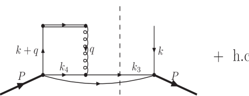
Figure 1: The leading contribution to the Sivers function $f_{1T}(x,k_{\perp})$ in the MIT bag model.

Using the identity,

$$\frac{1}{q^{+}-i\epsilon}-\frac{1}{q^{+}+i\epsilon}=i(2\pi)\delta(q^{+})\ ,$$ (16)

we get

$$f_{1T}^{\perp\alpha}(x,k_{\perp}) = -2g^{2}\frac{ME_{P}}{k^{y}}\int\frac{d^{2}q_{\perp}}{(2\pi)^{5}}\frac{i}{q^{2}}\sum\limits_{\beta,m_{1},m_{2},m_{3},m_{4}}T^{a}_{ij}T^{a}_{kl}\langle PS_{x}|b_{\alpha m_{1}}^{i\dagger}b_{\alpha m_{2}}^{j}b_{\beta m_{3}}^{k\dagger}b_{\beta m_{4}}^{l}|PS_{x}\rangle$$ (17)

$$~{}~{}\times\varphi_{m_{1}}^{\dagger}(\vec{k}-\vec{q}_{\perp})\gamma^{0}\gamma^{+}\varphi_{m_{2}}(\vec{k})\int\frac{d^{3}k_{3}}{(2\pi)^{3}}\varphi_{m_{3}}^{\dagger}(\vec{k_{3}})\gamma^{0}\gamma^{+}\varphi_{m_{4}}(\vec{k_{3}}-\vec{q}_{\perp})\ .$$

The $k_{3}$ integration only depends on $q$, and so we can write this integral as a function of $q^{2}$, and define

$$\int\frac{d^{3}k_{3}}{(2\pi)^{3}}\varphi_{m_{3}}^{\dagger}(\vec{k_{3}})\gamma^{0}\gamma^{+}\varphi_{m_{4}}(\vec{k_{3}}-\vec{q})\equiv\frac{1}{\sqrt{2}}F(q^{2})\delta_{m_{3}m_{4}}\ .$$ (18)

The function $F(q^{2})$ is

$$F(q^{2}) = \frac{16\omega^{4}}{\pi^{2}j_{0}^{2}(\omega)(\omega-1)}\frac{1}{M_{P}^{2}}\int d^{3}k_{3}\left[t_{0}(|\vec{k}_{3}|)t_{0}(|\vec{k}_{3}^{\prime}|)+\frac{k_{3}^{\prime z}}{|\vec{k}_{3}^{\prime}|}t_{0}(|\vec{k}_{3}|)t_{1}(|\vec{k}_{3}^{\prime}|)\right.$$ (19)

$$\left.+\frac{k_{3}^{z}}{|\vec{k}_{3}|}t_{1}(|\vec{k}_{3}|)t_{0}(|\vec{k}_{3}^{\prime}|)+\frac{\vec{k}_{3}\cdot\vec{k}_{3}^{\prime}}{|\vec{k}_{3}||\vec{k}_{3}^{\prime}|}t_{1}(|\vec{k}_{3}|)t_{1}(|\vec{k}_{3}^{\prime}|)\right]\ ,$$

where $\vec{k}_{3}^{\prime}=\vec{k}_{3}+\vec{q}$. It is easy to show that $F(q^{2})\rightarrow 1$ as $q^{2}\rightarrow 0$.

With $F(q^{2})$, we can further simplify Eq. (17) as,

$$f_{1T}^{\perp\alpha}(x,k_{\perp}) = -\sqrt{2}g^{2}C_{\alpha}^{\prime}(S_{x})\frac{ME_{P}}{k^{y}}\int\frac{d^{2}q_{\perp}}{(2\pi)^{5}}F(q^{2})\frac{i}{q^{2}}\varphi_{m_{1}}^{\dagger}(\vec{k}-\vec{q}_{\perp})\gamma^{0}\gamma^{+}\varphi_{m_{2}}(\vec{k})\ ,$$ (20)

and $C_{\alpha}^{\prime}$ is

$$C_{\alpha}^{\prime}(S_{x}) = \sum\limits_{\beta,m_{3},m_{4}}\delta_{m_{3}m_{4}}T^{a}_{ij}T^{a}_{kl}\langle PS_{x}|b_{\alpha m_{1}}^{i\dagger}b_{\alpha m_{2}}^{j}b_{\beta m_{3}}^{k\dagger}b_{\beta m_{4}}^{l}|PS_{x}\rangle$$ (21)

$$= \frac{\delta_{m_{1}+m_{2}}}{2}C_{\alpha}\ ,$$

where $\delta_{m_{1}+m_{2}}$ factor comes from the fact that the proton is polarized along the $\hat{x}$ direction, and $C_{\alpha}$ is defined as

$$C_{\alpha}=\sum\limits_{\beta,m_{1},m_{3}}T^{a}_{ij}T^{a}_{kl}\langle PS_{x}|b_{\alpha m_{1}}^{i\dagger}b_{\alpha-m_{1}}^{j}b_{\beta m_{3}}^{k\dagger}b_{\beta m_{3}}^{l}|PS_{x}\rangle\ .$$ (22)

Substituting the above results into Eq. (20), we find

$$f_{1T}^{\perp\alpha}(x,k_{\perp})=-\sqrt{2}g^{2}C_{\alpha}\frac{ME_{P}}{k^{y}}\int\frac{d^{2}q_{\perp}}{(2\pi)^{5}}F(q^{2})\frac{i}{q^{2}}\frac{1}{2}\sum\limits_{m}\varphi_{m}^{\dagger}(\vec{k}-\vec{q}_{\perp})\gamma^{0}\gamma^{+}\varphi_{-m}(\vec{k})\ .$$ (23)

From the bag model wave functions, we obtain

$$\varphi_{m}^{\dagger}(\vec{k}^{\prime})\gamma^{0}\gamma^{+}\varphi_{-m}(\vec{k}) = \frac{4\pi^{2}R_{0}^{6}}{\sqrt{2}}i\chi_{m}^{\dagger}\left[\frac{(\vec{\sigma}\times\vec{k}^{\prime})^{z}}{|\vec{k}^{\prime}|}t_{1}(k^{\prime})t_{0}(k)-\frac{(\vec{\sigma}\times\vec{k})^{z}}{|\vec{k}|}t_{0}(k^{\prime})t_{1}(k)\right.$$ (24)

$$\left.+\frac{\vec{k}\times\vec{q}_{\perp}\cdot\vec{\sigma}}{|\vec{k}^{\prime}||\vec{k}|}t_{1}(k^{\prime})t_{1}(k)\right]\chi_{-m}\ ,$$

where $\vec{k}^{\prime}=\vec{k}-\vec{q}_{\perp}$. Because the proton is polarized along the $\hat{x}$ direction, in the above equation, only the $\sigma_{x}$ terms contribute, and the $q_{\perp}$ integral will be proportional to $k^{y}$. And finally, we get

$$f_{1T}^{\perp\alpha}(x,k_{\perp}) = -\frac{16\omega^{4}g^{2}C_{\alpha}}{\pi^{2}j_{0}^{2}(\omega)(\omega-1)}\frac{1}{M_{P}}\left[I_{0}(x,k_{\perp})-I_{1}(x,k_{\perp})\right]\ .$$ (25)

The two integrals $I_{0}$ and $I_{1}$ are defined as

$$I_{0}(x,k_{\perp}) = \int\frac{d^{2}q_{\perp}}{(2\pi)^{2}}\frac{F(q_{\perp}^{2})}{q_{\perp}^{2}}\left[\frac{t_{1}(k^{\prime})t_{0}(k)}{k^{\prime}}-\frac{t_{0}(k^{\prime})t_{1}(k)}{k}\right]\ ,$$

$$I_{1}(x,k_{\perp}) = \left[t_{0}(k)+\frac{k_{z}}{k}t_{1}(k)\right]\int\frac{d^{2}q_{\perp}}{(2\pi)^{2}}\frac{F(q_{\perp}^{2})}{q_{\perp}^{2}}\frac{t_{1}(k^{\prime})}{k^{\prime}}\frac{\vec{k}_{\perp}\cdot\vec{q}_{\perp}}{k_{\perp}^{2}}\ ,$$ (26)

where $k_{z}=xM_{p}-\varepsilon$, $k=\sqrt{(xM_{P}-\varepsilon)^{2}+k_{\perp}^{2}}$ with $\varepsilon=\omega/R_{0}$, and $k^{\prime}=\sqrt{(xM_{P}-\varepsilon)^{2}+(\vec{k}_{\perp}-\vec{q}_{\perp})^{2}}$. $R_{0}$ and $M_{P}$ are bag radius and proton mass, respectively. In our calculations, we fix the dimensionless parameter $R_{0}M_{P}=4\omega$.

Working out the matrix elements of Eq. (22) for the valence quarks, we find

$$C_{u}=-\frac{16}{9},~{}~{}~{}~{}C_{d}=\frac{4}{9}\ ,$$ (27)

for up and down quarks respectively, which means that the up quark and down quark have opposite signs for the Sivers function, and differ by a factor of 4. This is the result of the $SU(6)$ wave function we used for the proton. For a polarized proton, the polarized up quark distribution has a factor of $4/3$ while down quark has $-1/3$. Phenomenologically, since $\pi^{+}$ production is dominated by the up quark fragmentation and $\pi^{0}$ is dominated by either the up quark or the down quark fragmentation, while $\pi^{-}$ is dominated by the down quark fragmentation, the above prediction will lead to larger single spin asymmetries for $\pi^{+}$ and $\pi^{0}$ than that for $\pi^{-}$ with opposite signs if assuming the Sivers mechanism. In this estimate, we have neglected the “unfavored” fragmentation contribution to the pion production, which has been shown to play an important role for $\pi^{-}$ asymmetry ma . Taking into account the “unfavored” ($u$ quark) fragmentation contribution which has opposite sign from the “favored” ($d$ quark) one, we will get even smaller asymmetry for $\pi^{-}$. We note that the HERMES collaboration actually showed much larger asymmetries for $\pi^{+}$ and $\pi^{0}$ than that for $\pi^{-}$ hermes . On the other hand, concerning the quark distribution in the neutron, one shall have 4 times larger Sivers function for down quark than that for up quark by isospin symmetry argument from the above results, and both of them will have different signs compared to the proton ones. That means, with the neutron target, one would have a factor of 2 smaller asymmetry for $\pi^{+}$ with opposite sign compared to the asymmetry with the proton target. It is interesting to note that JLab will measure these asymmetries with the proton target, and the neutron target as well. The comparison of the SSA between the proton and neutron targets will provide crucial test on the Sivers mechanism for the SSA.

Figure 2: The Sivers functions $f_{1T}^{\perp}(x,k_{\perp})$ for the valence quarks at $x=0.3$ as functions of $k_{\perp}$, where the quark-gluon coupling $\alpha_{s}=0.2$.

In Fig. 2, we plot the Sivers functions for up and down quarks as functions of transverse momentum $k_{\perp}$ at $x=0.3$. Here the quark-gluon coupling $g$ is treated as a free parameter, and we set $\alpha_{s}=g^{2}/4\pi=0.2$, which is smaller than the value used in mitbag to determine the mass splitting of baryons. Since bag model is not suitable for the calculation of the distribution at large transverse momentum, here we only show the results for the range of $k_{\perp}$ smaller than $0.7$GeV.

The contribution from the Sivers effect to the SSA in the semi-inclusive process can be calculated from the above results divided by the unpolarized quark distribution in the same model bag-pdf . The asymmetry ${\cal P}_{y}$ is calculated as

$${\cal P}_{y}=\frac{k_{\perp}^{x}}{M}f_{1T}^{\perp}(x,k_{\perp})/f_{1}(x,k_{\perp})\ ,$$ (28)

where the polarization of the proton is along the $\hat{y}$ direction. We plot these asymmetries for the valence quarks as functions of $k_{\perp}^{x}$ at $x=0.3$ in Fig. 3(a), and as functions of $x$ at $k_{\perp}^{x}=0.5$ in Fig. 3(b). These asymmetries are for the quark distributions. To get the asymmetry associated with the hadron production in semi-inclusive processes, we need to convolute the above results with the fragmentation functions of the hadrons.

Figure 3: The bag model prediction for the asymmetry of the quark distribution in a transverse polarized proton as a function of $k^{x}$ and $x$, where $\alpha_{s}=0.2$.

It is also interested to study the moments of the Sivers distribution. For example, one interested moment is defined as evolution

$$f_{1T}^{\perp(1)}(x)=\int d^{2}k_{\perp}\left(\frac{\vec{k}_{\perp}^{2}}{2M^{2}}\right)f_{1T}^{\perp}(x,k_{\perp})\ .$$ (29)

The numerical results for the above functions depending on $x$ are shown in Fig. 4, which can be fit with the following functional form,

$$f_{1T}^{\perp(1)u}(x) = -0.75x^{1.63}(1-x)^{4.06}\ ,$$

$$f_{1T}^{\perp(1)d}(x) = 0.19x^{1.63}(1-x)^{4.06}\ .$$ (30)

Since the bag model is not good for small $x$ parton distributions, we have abandoned the use of small $x$ points in the fit. As an illustration, we also plot the above fit for the up-quark in Fig. 4.

Figure 4: The first moments of the Sivers functions $f_{1T}^{(1)}(x)$ for valence quarks, where $\alpha_{s}=0.2$.

We can repeat the above calculations for another TMD parton distribution, $h_{1}^{\perp}$, which represents the correlation between the quark’s transverse momentum and polarization in an unpolarized proton state. It can be calculated from the expansion of the density matrix,

$${\cal M}=\frac{1}{2M}\left[h_{1}^{\perp}(x,k_{\perp})\sigma^{\mu\nu}k_{\mu}p_{\nu}+\dots\right]\ .$$ (31)

Inverting the above equation, we get

$$h_{1}^{\perp}(x,k_{\perp}) = \frac{M}{2\epsilon^{ij}k^{j}}\int\frac{d\xi^{-}d\xi_{\perp}}{(2\pi)^{3}}e^{-i(\xi^{-}k^{+}-\vec{\xi}_{\perp}\cdot\vec{k}_{\perp})}$$ (32)

$$\times\langle P|\overline{\psi}(\xi^{-},\xi_{\perp}){\cal L}^{\dagger}(\xi^{-},\xi_{\perp})\gamma^{+}\gamma^{i}\gamma_{5}{\cal L}(0,0_{\perp})\psi(0)|P\rangle\ ,$$

where the proton is unpolarized. Without the gauge link contribution, this function vanishes, as the Sivers function does. Expanding the gauge link to next-to-leading order, we get

$$h_{1\alpha}^{\perp}(x,k_{\perp}) = \frac{M}{2\epsilon^{ij}k^{j}}\int\frac{d\xi^{-}d\xi_{\perp}}{(2\pi)^{3}}e^{-i(\xi^{-}k^{+}-\vec{\xi}_{\perp}\cdot\vec{k}_{\perp})}$$ (33)

$$\times\langle P|\overline{\psi}_{\alpha i}(\xi^{-},\xi_{\perp})(ig)\int\limits_{\xi^{-}}^{\infty}d\eta^{-}A^{+}_{a}(\eta^{-},\xi_{\perp})T^{a}_{ij}\gamma^{+}\gamma^{i}\gamma_{5}\psi_{\alpha j}(0)|P\rangle+h.c.\ .$$

where the nucleon is unpolarized.

Using the same method as we did in the calculations of the Sivers function, we find that

$$h_{1\alpha}^{\perp}(x,k_{\perp}) = -\sqrt{2}g^{2}D_{\alpha}\frac{ME_{P}}{\epsilon^{ij}k^{j}}\int\frac{d^{2}q_{\perp}}{(2\pi)^{5}}F(q^{2})\frac{i}{q^{2}}\varphi_{m}^{\dagger}(\vec{k}-\vec{q}_{\perp})\gamma^{0}\gamma^{+}\gamma^{i}\gamma_{5}\varphi_{m}(\vec{k})\ ,$$ (34)

where $D_{\alpha}$ is defined as

$$D_{\alpha}=\sum\limits_{\beta,m_{1}m_{3}}T^{a}_{ij}T^{a}_{kl}\langle P|b_{\alpha m_{1}}^{i\dagger}b_{\alpha m_{1}}^{j}b_{\beta m_{3}}^{k\dagger}b_{\beta m_{3}}^{l}|P\rangle\ .$$ (35)

And finally, we can write the distribution $h_{1}^{\perp}$ in the form of,

$$h_{1\alpha}^{\perp}(x,k_{\perp}) = -\frac{16\omega^{4}g^{2}D_{\alpha}}{\pi^{2}j_{0}^{2}(\omega)(\omega-1)}\frac{1}{M_{P}}\left[I_{0}(x,k_{\perp})-I_{1}(x,k_{\perp})\right]\ ,$$ (36)

which is the same as Eq. (25) except the color factor. For the valence quark distributions, we have

$$D_{u}=-\frac{8}{3},~{}~{}~{}~{}~{}D_{d}=-\frac{4}{3},$$ (37)

which means that the up and down quarks have the same sign for $h_{1}^{\perp}$ distribution, and differ by a factor of two. For the unpolarized proton, the up quark distribution is two times larger than down quark distribution. This prediction shows that the asymmetries associated with $h_{1}^{\perp}$ for $\pi^{\pm}$ and $\pi^{0}$ will have the same sign. This is quite different from the asymmetries associated with the Sivers function $f_{1T}^{\perp}$ we discussed before. For the neutron, one has the similar prediction.

As an illustration, we plot in Fig. 5 the distributions $h_{1}^{\perp}(x,k_{\perp})$ as functions of transverse momentum at $x=0.3$. We can also calculate the moments of the $h_{1}^{\perp}$ functions for up quark and down quark, and fit with the following parameterizations,

$$h_{1}^{\perp(1)u}(x)=-1.13x^{1.63}(1-x)^{4.06}\ ,$$

$$h_{1}^{\perp(1)d}(x)=-0.56x^{1.63}(1-x)^{4.06}\ ,$$ (38)

where the same functional dependence as $f_{1T}^{\perp(1)}$ have been observed.

Figure 5: $h_{1}^{\perp}(x,k_{\perp})$ for the valence quarks at $x=0.3$ as functions of $k_{\perp}$, where $\alpha_{s}=0.2$.

In conclusion, we have calculated the Sivers function in the MIT bag model. The gauge link in the gauge-invariant definition of the TMD parton distribution functions plays the crucial role for the nonvanishing of the Sivers function. Our calculations show that the up quark Sivers function is 4 times larger than that of down quark with opposite signs, consistent with the $SU(6)$ spin-flavor structure of the proton. These results lead to testable consequence for the single spin asymmetry associated with the Sivers function in the semi-inclusive deep inelastic pion productions: the asymmetries for $\pi^{+}$ and $\pi^{0}$ will be larger than that for $\pi^{-}$, and with different signs. Distribution $h_{1}^{\perp}$ has also been calculated in the same model, and we found that the up quark and down quark have the same sign, which means that the asymmetries associated with this distribution for $\pi^{\pm}$ and $\pi^{0}$ will have the same sign.

We end up our paper with a few comments. First, in our calculations, we have used free gluon propagator connecting gluon fields inside the bag, which is an approximation bag-dynamics . Secondly, we have ignored the scale evolution of the Sivers function moments $f_{1T}^{\perp(1)}(x,Q^{2})$ and $h_{1}^{\perp(1)}(x,Q^{2})$ evolution ; andrei1 . Our calculations are performed at the bag scale, which is much lower than typical hard scattering scales. However, the evolution of these functions is not clear yet andrei1 ; Goe03 , and is beyond the scope of the present paper.

The author thanks Andrei Belitsky and Xiangdong Ji for their suggestions and useful comments and critical readings of the manuscript. The author also thanks Harut Avagyan, Stan Brodsky, Matthias Burkardt, Xiaodong Jiang, and Mark Strikman for their comments. We thank the Department of Energy’s Institute for Nuclear Theory at the University of Washington for its hospitality during the program “Generalized parton distributions and hard exclusive processes” and the Department of Energy for the partial support during the completion of this paper. This work was supported by the U. S. Department of Energy via grants DE-FG02-93ER-40762.

References

• (1) A. Airapetian et al. [HERMES Collaboration], Phys. Rev. Lett.  84, 4047 (2000) [arXiv:hep-ex/9910062]; A. Airapetian et al. [HERMES Collaboration], Phys. Rev. D 64, 097101 (2001) [arXiv:hep-ex/0104005].
• (2) D. Adams et al. [Spin Muon Collaboration (SMC)], Phys. Lett. B 336, 125 (1994) [arXiv:hep-ex/9408001]; A. Bravar [Spin Muon Collaboration], Nucl. Phys. A 666, 314 (2000).
• (3) H. Avakian [CLAS Collaboration], proceedings of ”Testing QCD Through SPIN Observables” (Ed.D.G.Crabb et al.) University of Virginia April 2002 (2002).
• (4) R. L. Jaffe and X. Ji, Phys. Rev. Lett. 67, 552 (1991); Nucl. Phys. B 375, 527 (1992).
• (5) J. C. Collins, Nucl. Phys. B 396, 161 (1993) [arXiv:hep-ph/9208213].
• (6) D. W. Sivers, Phys. Rev. D 41, 83 (1990) [Annals Phys.  198, 371 (1990)]; D. W. Sivers, Phys. Rev. D 43, 261 (1991).
• (7) P. J. Mulders and R. D. Tangerman, Nucl. Phys. B 461, 197 (1996) [Erratum-ibid. B 484, 538 (1997)] [arXiv:hep-ph/9510301]. D. Boer and P. J. Mulders, Phys. Rev. D 57, 5780 (1998) [arXiv:hep-ph/9711485].
• (8) M. Anselmino, M. Boglione, and F. Murgia, Phys. Lett. B 362, 164 (1995); M. Anselmino and F. Murgia, Phys. Lett. B 442, 470 (1998).
• (9) S. J. Brodsky, D. S. Hwang and I. Schmidt, Phys. Lett. B 530, 99 (2002) [arXiv:hep-ph/0201296]; Nucl. Phys. B 642, 344 (2002) [arXiv:hep-ph/0206259].
• (10) J. C. Collins, Phys. Lett. B 536, 43 (2002) [arXiv:hep-ph/0204004].
• (11) X. Ji and F. Yuan, Phys. Lett. B 543, 66 (2002) [arXiv:hep-ph/0206057].
• (12) A. V. Belitsky, X. Ji and F. Yuan, Nucl. Phys. B 656, 165 (2003) [arXiv:hep-ph/0208038].
• (13) D. Boer, P. J. Mulders and F. Pijlman, arXiv:hep-ph/0303034.
• (14) J. w. Qiu and G. Sterman, Phys. Rev. Lett.  67, 2264 (1991); Phys. Rev. D 59, 014004 (1999) [arXiv:hep-ph/9806356].
• (15) see for example reviews, M. Anselmino, A. Efremov and E. Leader, Phys. Rept.  261, 1 (1995) [Erratum-ibid.  281, 399 (1997)] [arXiv:hep-ph/9501369]; V. Barone, A. Drago and P. G. Ratcliffe, Phys. Rept.  359, 1 (2002) [arXiv:hep-ph/0104283].
• (16) M. Burkardt, Phys. Rev. D 66, 114005 (2002) [arXiv:hep-ph/0209179]; arXiv:hep-ph/0302144.
• (17) J. C. Collins and D. E. Soper, Nucl. Phys. B 193, 381 (1981), [Erratum-ibid. B 213, 545 (1983).] ; J. C. Collins and D. E. Soper, Nucl. Phys. B 194, 445 (1982).
• (18) X. Ji, J. P. Ma and F. Yuan, Nucl. Phys. B 652, 383 (2003) [arXiv:hep-ph/0210430].
• (19) D. Boer, S. J. Brodsky and D. S. Hwang, Phys. Rev. D 67, 054003 (2003) [arXiv:hep-ph/0211110]; S. J. Brodsky, D. S. Hwang and I. Schmidt, Phys. Lett. B 553, 223 (2003) [arXiv:hep-ph/0211212].
• (20) L. P. Gamberg, G. R. Goldstein and K. A. Oganessyan, arXiv:hep-ph/0301018.
• (21) A. Chodos, R. L. Jaffe, K. Johnson, C. B. Thorn and V. Weisskopf, Phys. Rev. D 9, 3471 (1974).
• (22) R. L. Jaffe, Phys. Rev. D 11, 1953 (1975); A. W. Schreiber, A. I. Signal and A. W. Thomas, Phys. Rev. D 44, 2653 (1991); R. L. Jaffe and X. Ji, Phys. Rev. D 43, 724 (1991); M. Stratmann, Z. Phys. C 60, 763 (1993).
• (23) M. Betz and R. Goldflam, Phys. Rev. D 28, 2848 (1983); X. Song and J. S. McCarthy, Phys. Rev. C 46, 1077 (1992).
• (24) T.H. Hansson and R.L. Jaffe, Phys. Rev. 28, 882 (1983).
• (25) B. Q. Ma, I. Schmidt and J. J. Yang, Phys. Rev. D 66, 094001 (2002); Phys. Rev. D 65, 034010 (2002); Phys. Rev. D 63, 037501 (2001).
• (26) A. A. Henneman, D. Boer and P. J. Mulders, Nucl. Phys. B 620, 331 (2002) [arXiv:hep-ph/0104271].
• (27) A. V. Belitsky, Phys. Lett. B 405, 312 (1997) [arXiv:hep-ph/9702356].
• (28) K. Goeke, A. Metz, P. V. Pobylitsa and M. V. Polyakov, arXiv:hep-ph/0302028.