Abstract

This study investigates the potential of the TESLA Linear Collider for measuring resonance parameters of Higgs bosons beyond the mass range studied so far.

The analysis is based on the reconstruction of events from the Higgsstrahlung process ${\mathrm{e^{+}}\mathrm{e^{-}}\to\mathrm{H}\mathrm{Z}}$. It is shown that the total width $\Gamma_{\mathrm{H}}$, the mass $m_{\mathrm{H}}$ and the event rate can be measured from the mass spectrum in a model independent fit. Also, the branching ratios $\mathrm{BR}_{\mathrm{H}\to\mathrm{W}\mathrm{W}}$ and $\mathrm{BR}_{\mathrm{H}\to\mathrm{Z}\mathrm{Z}}$ can be measured, assuming these are the only relevant Higgs decay modes.

The simulation includes realistic detector effects and all relevant Standard Model background processes. Results are given for $m_{\mathrm{H}}=200-320\,\mathrm{GeV}$ assuming ${\cal\int\!\!L}=500\,\mathrm{fb}^{-1}$ integrated luminosity at collision energies of $\sqrt{s}=500\,\mathrm{GeV}$.

1 Introduction

During the past years many simulations have been performed to investigate the prospects of measuring Higgs boson properties at future Linear Colliders [1, 2, 3]. The main focus was set to Higgs masses $m_{\mathrm{H}}$ below the $\mathrm{W}\mathrm{W}$-threshold which is the mass region prefered by recent electroweak data.

In high energy $\mathrm{e^{+}e^{-}}$ collisions Higgs bosons can be produced in two dominant production processes: Higgsstrahlung $\mathrm{e^{+}e^{-}}\to\mathrm{H}\mathrm{Z}$ and $\mathrm{W}\mathrm{W}$-fusion $\mathrm{e^{+}e^{-}}\to\mathrm{H}\nu_{\mathrm{e}}\bar{\nu_{\mathrm{e}}}$, see Fig. 1. For lower collision energies $\sqrt{s}$, Higgsstrahlung with $\sigma_{\mathrm{H}\mathrm{Z}}\sim 1/s$ dominates, while $\mathrm{W}\mathrm{W}$-fusion becomes the major production mode due its $\sigma_{\mathrm{H}\nu_{\mathrm{e}}\bar{\nu_{\mathrm{e}}}}\sim\log s$ cross-section rise if $\sqrt{s}$ is large compared to $m_{\mathrm{H}}$. The cross sections of both processes for the considered range of Higgs masses are plotted in Fig. 2.

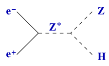
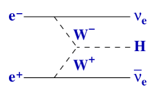
Figure 1: Higgs production diagrams: Higgsstrahlung (left) and $\mathrm{W}\mathrm{W}$-fusion (right).

Higgs bosons couple to mass and therefore decay in general to the heaviest particles possible. In the Standard Model (SM) and most of its extensions, the total Higgs decay width is expected to be very small for Higgs masses below the $\mathrm{W}\mathrm{W}$-threshold. Fig. 3 shows the SM prediction. Only if the Higgs width is as large as few $\mathrm{GeV}$ can it be determined from the observed Higgs lineshape. This is not possible for smaller widths due to limited detector resolution, but the width can only be determined indirectly via the Higgs couplings [6, 7].

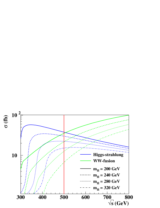
Figure 2: Higgs production cross sections as predicted by the Standard Model. Values are calculated using HZHA [4].

From the lineshape not only the width, but also the mass and event rate can be determined in a model-independent way. The signal and background processes studied are specified in Sec. 2. Event selection is described in Sec. 3 followed by the methods of estimating detector resolution in Sec. 4. For this, a separation of $\mathrm{H}\to\mathrm{W}\mathrm{W}$ and $\mathrm{H}\to\mathrm{Z}\mathrm{Z}$ decays is necessary, which can be interpreted as branching fraction measurements assuming that there are no other major decay modes. The note continues with details on the reconstruction of Higgs resonance parameters in Sec. 5. Results are summarized and discussed in Sec. 6.

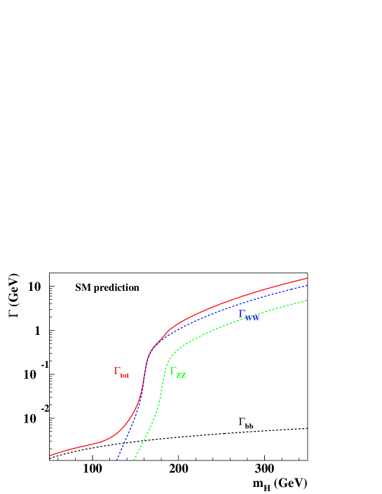
Figure 3: Standard Model prediction for the total Higgs width $\Gamma_{\mathrm{tot}}$. Also shown are the partial widths $\Gamma_{\mathrm{b}\mathrm{\bar{\mathrm{b}}}}$, $\Gamma_{\mathrm{W}\mathrm{W}}$ and $\Gamma_{\mathrm{Z}\mathrm{Z}}$ of the dominant decay modes. Values are calculated using HDECAY [5].

2 Signal and Background

Higgs bosons with Standard Model couplings are studied. The parameter space of interest ranges from $m_{\mathrm{H}}=200\,\mathrm{GeV}$ to $320\,\mathrm{GeV}$, where both cross section and width are large enough for precision measurements.

SM Higgs bosons in the mass range under study, decay almost exclusively to pairs of massive gauge bosons. The final state of interest therefore is $\mathrm{e^{+}e^{-}}\to\mathrm{H}\,(\mathrm{Z})\to\mathrm{W}\mathrm{W}/\mathrm{Z}\mathrm{Z}\,(\mathrm{Z})$. All successive decay modes are listed in Tab. 1.

		$\mathrm{H}\to$		SM branching	Events
	Final state	$\mathrm{W}\mathrm{W}$	$\,\;\mathrm{Z}\mathrm{Z}\;\,$	fraction	per $500\,\mathrm{fb}^{-1}$
1.	$2\nu+X$	$\times$	$\times$	35.08 %	6145
2.	$\mathrm{q}\mathrm{q}\,\mathrm{q}\mathrm{q}\,\mathrm{q}\mathrm{q}$	$\times$	$\times$	34.3 %	6000
3.	$\mathrm{q}\mathrm{q}\,\mathrm{q}\mathrm{q}\,\ell\nu$	$\times$		19.18 %	3355
4.	$\ell\ell\,\mathrm{q}\mathrm{q}\,\mathrm{q}\mathrm{q}$	$\times$	$\times$	7.84 %	1370
5.	$\ell\ell\,\mathrm{q}\mathrm{q}\,\ell\nu$	$\times$		2.94 %	515
6.	$\ell\ell\,\ell\ell\,\mathrm{q}\mathrm{q}$		$\times$	0.63 %	110
7.	$\ell\ell\,\ell\ell\,\ell\ell$		$\times$	0.03 %	5

Table 1: Signal final states and their occurrence. Numbers given are estimates using $\mathrm{BR}_{\mathrm{H}\to\mathrm{W}\mathrm{W}}=0.7$, $\mathrm{BR}_{\mathrm{H}\to\mathrm{Z}\mathrm{Z}}=0.3$, $\mathrm{BR}_{\mathrm{W}\to\ell\nu}=\mathrm{BR}_{\mathrm{Z}\to\ell\ell}=0.3$, $\mathrm{BR}_{\mathrm{W}\to\mathrm{q}\mathrm{q}}=\mathrm{BR}_{\mathrm{Z}\to\mathrm{q}\mathrm{q}}=0.7$ and $\sigma_{\mathrm{H}\mathrm{Z}}=35\,\mathrm{fb}$ as predicted by the SM for $m_{\mathrm{H}}=240\,\mathrm{GeV}$. Here, $\ell$ is any charged lepton flavor and $\mathrm{q}$ any quark flavor kinematically allowed.

Approximately one third of the $\mathrm{H}\mathrm{Z}$-events contain more than one neutrino and thus a precise mass reconstruction is difficult. For the rest, the fully hadronic final state is by far dominant. But also, this is the channel where the largest background contributions are expected (e.g. $\mathrm{e^{+}e^{-}}\to\mathrm{t}\mathrm{\bar{\mathrm{t}}}$). The same is true for the next-to-dominant decay mode (hadronic $\mathrm{Z}$-decay plus semi-leptonic decay of the $\mathrm{W}$-pair). On the contrary, the gold-plated channel with six leptons in the final state is too rare for precision measurements. Channel 4 with one leptonic $\mathrm{Z}$-decay and hadronic $\mathrm{W}$- or $\mathrm{Z}$-pair decays is a good compromise between signal rate and background contamination.

Since $\tau$-decays always include neutrinos, only $\ell=\mathrm{e},\,\mu$ are considered to achieve the best mass reconstruction. So, from here on lepton only means electron or muon.

All background processes with two charged leptons plus jets are considered. They can be classified as follows:

• Six fermion proceses, $\mathrm{e^{+}}\mathrm{e^{-}}\to 2\ell\;4\mathrm{q}$, yield events with the same final state as signal events. As will be shown later, this is the dominant class of background processes.

• Four fermion processes including $\mathrm{Z}\mathrm{Z}$-pair production, $\mathrm{e^{+}}\mathrm{e^{-}}\to 2\ell\;2\mathrm{q}$. First of all, this class of processes is problematic because of huge cross sections. However, event topology differs from signal events.

• Top quark pair production, $\mathrm{e^{+}e^{-}}\to\mathrm{t}\mathrm{\bar{\mathrm{t}}}\to\mathrm{b}\mathrm{\bar{\mathrm{b}}}\mathrm{W}^{+}\mathrm{W}^{-}$. Here, high energetic leptons might not only occur in $\mathrm{W}$- but also in $\mathrm{b}$-decays. Therefore, all decays $\mathrm{W}\to\mathrm{q}\mathrm{\bar{\mathrm{q}}}$ and $\mathrm{W}\to\ell\nu$ are considered. Again it is not event topology but large cross section which makes this backgroud possibly dangerous.

Other processes (e.g. $\mathrm{e^{+}e^{-}}\to\mathrm{W}\mathrm{W}\to\mathrm{q}\mathrm{q}\ell\nu$) are expected to be negligible due to missing isolated leptons, large missing energy or low mass of the hadronic system.

Signal as well as background events are generated using WHiZard 1.22 [8], except $\mathrm{t}\mathrm{\bar{\mathrm{t}}}$-events for which PYTHIA 6.2 [9] is used. Both initial state radiation ISR and beamstrahlung [10] are taken into account. For this analysis, no significant signal over background enhancement is expected for polarized beams, so the possibility of beam polarization is not studied. Cuts on fermion-pair invariant masses $m_{\ell\ell}/m_{\mathrm{q}\mathrm{q}}>10\,\mathrm{GeV}$ for any lepton-/quark-pair are applied on MC level to save CPU power. These events anyhow are far from the parameter space of interest.

Detector response is simulated using the fast Monte Carlo SIMDET 4 [11] which parameterizes detector performance as described in the TESLA TDR [1].

3 Event Selection

In all events, energy flow objects, which are classified as lepton (electron or muon) are searched for. The most energetic of these objects is combined with any other identified lepton. The pair with invariant mass closest to $m_{\mathrm{Z}}$ is selected as $\mathrm{Z}\to\ell\ell$ candidate and removed from the event. All other energy flow objects are forced to four jets by the Durham recombination scheme [12].

The distributions of the most important variables used for background suppression are displayed in Fig. 4. Each event is required to pass the following cuts:

1. The event must contain at least two energy flow objects classified as electron or muon by the detector reconstruction, $N_{\ell}\geq 2$.

2. Both leptons from the $\mathrm{Z}$-decay must satisfy $\left|\cos\theta_{\ell}\right|<0.99$, where $\cos\theta_{\ell}$ is the lepton’s polar angle.

3. All jets must satisfy $\left|\cos\theta_{\mathrm{jet}}\right|<0.95$.

4. The two lepton invariant mass must be close to the $\mathrm{Z}$-mass, $\left|m_{\ell\ell}-m_{\mathrm{Z}}\right|<5\,\mathrm{GeV}$. This reduces background events with non-resonant lepton pairs.

5. The sum of the energy of both leptons must be significantly less than the beam energy, $E_{\ell\ell}<225\,\mathrm{GeV}=0.45\,\sqrt{s}$. In events from $\mathrm{Z}$-pair production, each $\mathrm{Z}$-boson carries half of the event energy, so events of this type are reduced.

6. The hadronic system must be four-jet like, $y_{34}>10^{-3}$. Here, $y_{34}$ is the separation parameter between three (small $y_{34}$) and four (large $y_{34}$) jets of the jet finder. This cut reduces most of the remaining four-fermion events with non-resonant leptons still left after the $m_{\ell\ell}$ cut.

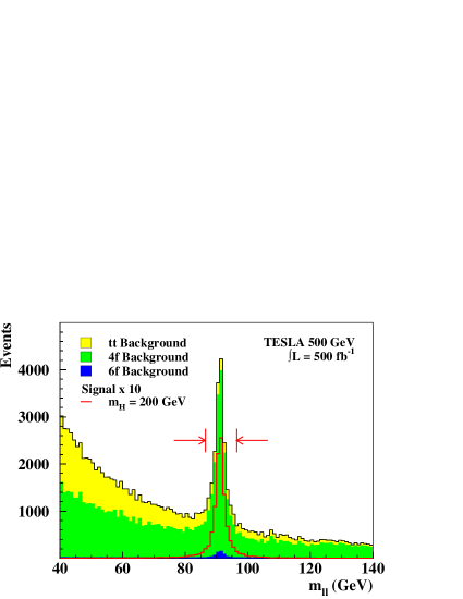
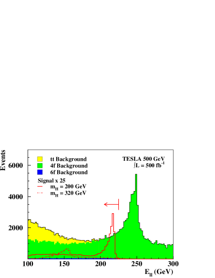
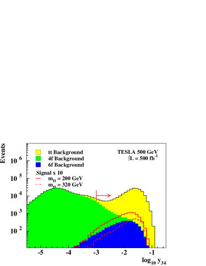
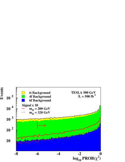
Figure 4: Distributions of the di-lepton mass $m_{\ell\ell}$, di-lepton energy $E_{\ell\ell}$, jet separation parameter $y_{34}$ and the $\chi^{2}$-probability of the kinematic fit $PROB(\chi^{2})$. Cuts are indicated by arrows.

In addition, a kinematic fit with four constraints is applied. The aim is to improve the mass resolution and to group the four jets into two pairs. The constraints are as follows:

1. Conservation of transverse momentum:
   $\sum p_{x}=0$, $\sum p_{y}=0$;

2. Conservation of energy and longitudinal momentum allowing for one initial hard photon in $\pm z$-direction:
   $(\sum E-\sqrt{s})^{2}-(\sum p_{z})^{2}=0$;

3. Four jets form two pairs of equal mass:
   $m_{1,2}=m_{3,4}$.

This fit is performed for all three possible assignements of the four jets to two pairs in the fourth constraint. The combination yielding the best fit $\chi^{2}$ is used. Events with a probability of this $\chi^{2}$ below $PROB(\chi^{2})<10^{-6}$ are rejected.

			Signal $m_{\mathrm{H}}\,[\mathrm{GeV}]$				Background
Variable (range)			200	240	280	320	6f	4f	$\mathrm{t}\mathrm{\bar{\mathrm{t}}}$
Events / $500\,\mathrm{fb}^{-1}$			1120	880	630	410	4340	392 000	240 000
1.-3.	$N_{\ell}$, $\cos{\theta_{\ell}}$, $\cos{\theta_{\mathrm{jet}}}$		904	706	498	322	1803	38 000	90 000
4.	$E_{ll}$	($<225\,\mathrm{GeV}$)	897	705	497	321	1512	5764	90 000
5.	$m_{ll}$	($m_{\mathrm{Z}}\pm 10\,\mathrm{GeV}$)	770	600	425	275	369	1506	750
6.	$y_{34}$	($>10^{-3}$)	745	581	413	268	343	5	357
7.	PROB($\chi^{2}$)	($>10^{-6}$)	585	463	333	216	271	0	4
Efficiency			52 %	53 %	53 %	53 %

Table 2: Evolution of event rates through the selection. Main remaining background source are events from 6f processes $\mathrm{e^{+}e^{-}}\to 2\ell\,4\mathrm{q}$. Event rates in the first line include MC level cuts as described in the text.

Tab. 2 shows the overall performance of the event selection. Background suppression is possible to $S/B\sim 1$ or better depending on the Higgs mass. Events from four fermion processes and $\mathrm{t}\mathrm{\bar{\mathrm{t}}}$-pair production can be rejected almost completely. Signal efficiency is stable as a function of $m_{\mathrm{H}}$ and lays above $\epsilon_{signal}>50\,\%$.

In the following, only three objects are considered per event: A reconstructed $\mathrm{Z}$-boson (the two leptons) and two further objects assumed to be either a pair of $\mathrm{W}$- or $\mathrm{Z}$-bosons (the jet pairs).

4 Separation of $\mathrm{H}\to\mathrm{W}\mathrm{W}$ and $\mathrm{H}\to\mathrm{Z}\mathrm{Z}$

Since it is a priori unknown which two of the three bosons originate from the Higgs decay, a distribution is formed which contains all three possible di-boson masses per event. It is expected that the correct pairing will exhibit a mass peak while the two wrong pairings will form a flat combinatorical background. The invariant di-boson mass spectrum is shown in Fig. 7, where the Higgs resonance is clearly visible for all Higgs masses.

In order to determine the resonance parameters ($m$, $\Gamma$, $N$) from this distribution, the theoretical Breit-Wigner shape of the resonance has to be convoluted with a properly tuned detector resolution function. The detector resolution is estimated by using MC with zero Higgs width, $\Gamma_{\mathrm{H}}=0$ and the same selection as described before.

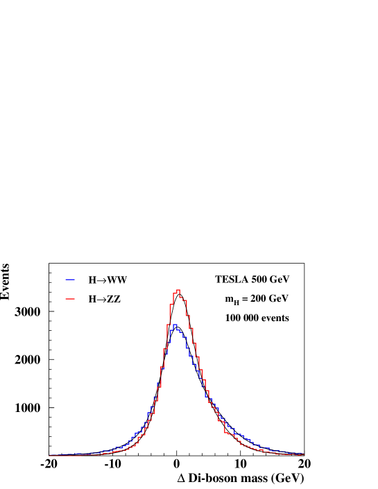
Figure 5: Di-boson mass resolution from MC with $\Gamma_{\mathrm{H}}=0\,\mathrm{GeV}$. As can be seen, resolutions differ for $\mathrm{H}\to\mathrm{W}\mathrm{W}$ and $\mathrm{H}\to\mathrm{Z}\mathrm{Z}$. Both distributions are asymmetric due to the constraints of the kinematic fit.

It turns out that this detector resolution is different for $\mathrm{H}\to\mathrm{W}\mathrm{W}$ and $\mathrm{H}\to\mathrm{Z}\mathrm{Z}$ decays, both of which enter the di-boson mass spectrum with relative fractions

$$RF_{\mathrm{H}\to\mathrm{W}\mathrm{W}}=\frac{N_{\mathrm{H}\to\mathrm{W}\mathrm{W}}}{N_{\mathrm{H}\to\mathrm{W}\mathrm{W}}+N_{\mathrm{H}\to\mathrm{Z}\mathrm{Z}}}\qquad\mathrm{and}\qquad RF_{\mathrm{H}\to\mathrm{Z}\mathrm{Z}}=\frac{N_{\mathrm{H}\to\mathrm{Z}\mathrm{Z}}}{N_{\mathrm{H}\to\mathrm{W}\mathrm{W}}+N_{\mathrm{H}\to\mathrm{Z}\mathrm{Z}}}$$

respectively, with $N$ being the number of events for each channel after selection. The different resolutions arise from the fact that for $\mathrm{H}\to\mathrm{Z}\mathrm{Z}$ the correct di-boson mass partially is an $\ell\ell\,\mathrm{q}\mathrm{q}$ invariant mass, while for $\mathrm{H}\to\mathrm{W}\mathrm{W}$ it is always $\mathrm{q}\mathrm{q}\,\mathrm{q}\mathrm{q}$. The different expected mass spectra and the parameterizations used for convolution are shown in Fig. 5 for $m_{\mathrm{H}}=200\,\mathrm{GeV}$. Resolutions for the other Higgs masses are similar.

The fractions $RF_{\mathrm{H}\to\mathrm{W}\mathrm{W}}$ and $RF_{\mathrm{H}\to\mathrm{Z}\mathrm{Z}}$ are determined from the di-jet mass as obtained from the kinematic fit. An example for $m_{\mathrm{H}}=200\,\mathrm{GeV}$ is shown in Fig. 6, where two peaks from $\mathrm{W}$- and $\mathrm{Z}$-decays respectively are clearly visible. However, the tails are overlapping.

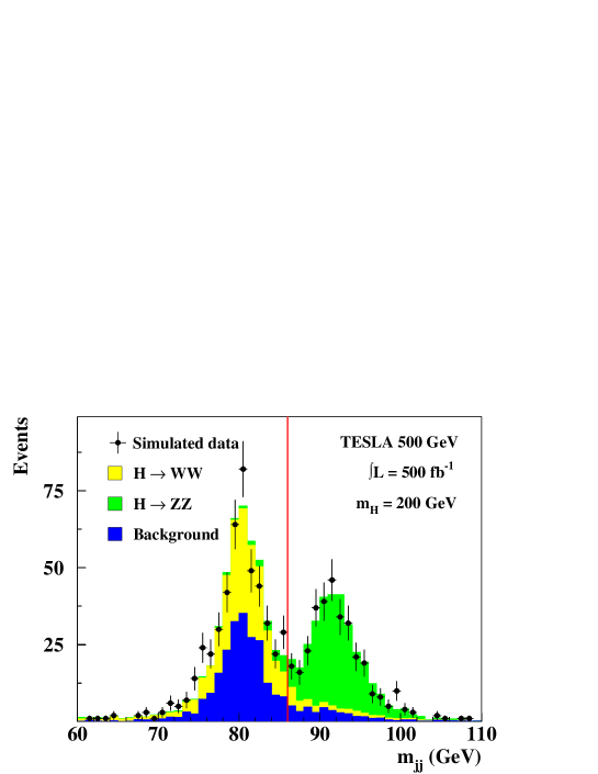
Figure 6: Jet-jet mass as obtained from the kinematic fit. Clearly visible are two peaks at $m_{\mathrm{W}}$ and $m_{\mathrm{Z}}$ respectively.

The di-jet mass spectrum is divided by a (in principle arbitrary) mass cut, choosen to be $m_{jj}=86\,\mathrm{GeV}$. The number of events from all event classes ($\mathrm{H}\to\mathrm{W}\mathrm{W}$, $\mathrm{H}\to\mathrm{Z}\mathrm{Z}$ and background), $N_{i}$ is broken up in $N_{i}^{-}$ events below and $N_{i}^{+}$ events above this cut. The corresponding probabilities are referred to as $P_{i}^{\pm}=N_{i}^{\pm}/N_{i}$. Expectations for $P_{i}^{\pm}$ and $N_{bkgrd}$ are derived from MC, while the total number $N_{tot}^{\pm}$ are counted in data.

From this, the relative fractions can be calculated according to:

$$N_{tot}^{+} = N_{bkgrd}^{+}+N_{\mathrm{H}\to\mathrm{W}\mathrm{W}}^{+}+N_{\mathrm{H}\to\mathrm{Z}\mathrm{Z}}^{+}$$

$$= N_{bkgrd}^{+}+N_{\mathrm{H}\to\mathrm{W}\mathrm{W}}\,P_{\mathrm{H}\to\mathrm{W}\mathrm{W}}^{+}+N_{\mathrm{H}\to\mathrm{Z}\mathrm{Z}}\,P_{\mathrm{H}\to\mathrm{Z}\mathrm{Z}}^{+}$$

$$= N_{bkgrd}^{+}+\left(N_{\mathrm{H}\to\mathrm{W}\mathrm{W}}+N_{\mathrm{H}\to\mathrm{Z}\mathrm{Z}}\right)\,\left(RF_{\mathrm{H}\to\mathrm{W}\mathrm{W}}\,P_{\mathrm{H}\to\mathrm{W}\mathrm{W}}^{+}+RF_{\mathrm{H}\to\mathrm{Z}\mathrm{Z}}\,P_{\mathrm{H}\to\mathrm{Z}\mathrm{Z}}^{+}\right)$$

$$= N_{bkgrd}^{+}+\left(N_{\mathrm{H}\to\mathrm{W}\mathrm{W}}+N_{\mathrm{H}\to\mathrm{Z}\mathrm{Z}}\right)\,\left(\left(1-RF_{\mathrm{H}\to\mathrm{Z}\mathrm{Z}}\right)\,P_{\mathrm{H}\to\mathrm{W}\mathrm{W}}^{+}+RF_{\mathrm{H}\to\mathrm{Z}\mathrm{Z}}\,P_{\mathrm{H}\to\mathrm{Z}\mathrm{Z}}^{+}\right).$$

With $N_{\mathrm{H}\to\mathrm{W}\mathrm{W}}+N_{\mathrm{H}\to\mathrm{Z}\mathrm{Z}}=N_{tot}-N_{bkgrd}$ resulting in

$$N_{tot}^{+} = N_{bkgrd}^{+}+\left(N_{tot}-N_{bkgrd}\right)\,\left(\left(1-RF_{\mathrm{H}\to\mathrm{Z}\mathrm{Z}}\right)\,P_{\mathrm{H}\to\mathrm{W}\mathrm{W}}^{+}+RF_{\mathrm{H}\to\mathrm{Z}\mathrm{Z}}\,P_{\mathrm{H}\to\mathrm{Z}\mathrm{Z}}^{+}\right)$$

$$\Longrightarrow\;RF_{\mathrm{H}\to\mathrm{Z}\mathrm{Z}} = \frac{N_{tot}^{+}-N_{bkgrd}^{+}}{\left(N_{tot}-N_{bkgrd}\right)\,\left(P_{\mathrm{H}\to\mathrm{Z}\mathrm{Z}}^{+}-P_{\mathrm{H}\to\mathrm{W}\mathrm{W}}^{+}\right)}-\frac{P_{\mathrm{H}\to\mathrm{W}\mathrm{W}}^{+}}{P_{\mathrm{H}\to\mathrm{Z}\mathrm{Z}}^{+}-P_{\mathrm{H}\to\mathrm{W}\mathrm{W}}^{+}}$$

$$\mathrm{and}\quad RF_{\mathrm{H}\to\mathrm{W}\mathrm{W}} = 1-RF_{\mathrm{H}\to\mathrm{Z}\mathrm{Z}}=\frac{N_{tot}^{-}-N_{bkgrd}^{-}}{\left(N_{tot}-N_{bkgrd}\right)\,\left(P_{\mathrm{H}\to\mathrm{W}\mathrm{W}}^{-}-P_{\mathrm{H}\to\mathrm{Z}\mathrm{Z}}^{-}\right)}-\frac{P_{\mathrm{H}\to\mathrm{Z}\mathrm{Z}}^{-}}{P_{\mathrm{H}\to\mathrm{W}\mathrm{W}}^{-}-P_{\mathrm{H}\to\mathrm{Z}\mathrm{Z}}^{-}}.$$

Due to the larger background contributions below the cut, the determination of $RF_{\mathrm{H}\to\mathrm{Z}\mathrm{Z}}$ and calculation of $RF_{\mathrm{H}\to\mathrm{W}\mathrm{W}}=1-RF_{\mathrm{H}\to\mathrm{Z}\mathrm{Z}}$ is more accurate than the opposite way. Nevertheless the analogue determination of $RF_{\mathrm{H}\to\mathrm{W}\mathrm{W}}$ by considering events below the threshold can be used as a cross-check.

The determination of the relative fractions is model independent. In addition, assuming there are only Higgs decays to $\mathrm{W}$- or $\mathrm{Z}$-pairs, the corresponding branching rations $\mathrm{BR}_{\mathrm{H}\to\mathrm{W}\mathrm{W}}$ and $\mathrm{BR}_{\mathrm{H}\to\mathrm{Z}\mathrm{Z}}$ can be calculated. For the calculation, the selection efficiencies $\epsilon_{\mathrm{H}\to\mathrm{W}\mathrm{W}}$ and $\epsilon_{\mathrm{H}\to\mathrm{Z}\mathrm{Z}}$ are taken from MC.

The number of events selected is a function of cross section, integrated luminosity, selection efficiency, and branching ratios. Consequently, the relative fraction $RF_{\mathrm{H}\to\mathrm{Z}\mathrm{Z}}$ can be expressed as

$$RF_{\mathrm{H}\to\mathrm{Z}\mathrm{Z}} = \frac{\sigma_{\mathrm{H}\mathrm{Z}}\,\,{\cal\int\!\!L}\,\,\epsilon_{\mathrm{H}\to\mathrm{Z}\mathrm{Z}}\,\,\mathrm{BR}_{\mathrm{H}\to\mathrm{Z}\mathrm{Z}}\,\,\mathrm{BR}_{\mathrm{Z}\mathrm{Z}\mathrm{Z}\to 2\ell\,4\mathrm{q}}}{\sigma_{\mathrm{H}\mathrm{Z}}\,\,{\cal\int\!\!L}\,\,(\epsilon_{\mathrm{H}\to\mathrm{Z}\mathrm{Z}}\,\,\mathrm{BR}_{\mathrm{H}\to\mathrm{Z}\mathrm{Z}}\,\,\mathrm{BR}_{\mathrm{Z}\mathrm{Z}\mathrm{Z}\to 2\ell\,4\mathrm{q}}+\epsilon_{\mathrm{H}\to\mathrm{W}\mathrm{W}}\,\,\mathrm{BR}_{\mathrm{H}\to\mathrm{W}\mathrm{W}}\,\,\mathrm{BR}_{\mathrm{Z}\mathrm{W}\mathrm{W}\to 2\ell\,4\mathrm{q}})}$$

$$= \frac{\epsilon_{\mathrm{H}\to\mathrm{Z}\mathrm{Z}}\,\,\mathrm{BR}_{\mathrm{H}\to\mathrm{Z}\mathrm{Z}}\,\,\mathrm{BR}_{\mathrm{Z}\mathrm{Z}\mathrm{Z}\to 2\ell\,4\mathrm{q}}}{\epsilon_{\mathrm{H}\to\mathrm{Z}\mathrm{Z}}\,\,\mathrm{BR}_{\mathrm{H}\to\mathrm{Z}\mathrm{Z}}\,\,\mathrm{BR}_{\mathrm{Z}\mathrm{Z}\mathrm{Z}\to 2\ell\,4\mathrm{q}}+\epsilon_{\mathrm{H}\to\mathrm{W}\mathrm{W}}\,\,\mathrm{BR}_{\mathrm{H}\to\mathrm{W}\mathrm{W}}\,\,\mathrm{BR}_{\mathrm{Z}\mathrm{W}\mathrm{W}\to 2\ell\,4\mathrm{q}}}.$$

With $\mathrm{BR}_{\mathrm{H}\to\mathrm{W}\mathrm{W}}+\mathrm{BR}_{\mathrm{H}\to\mathrm{Z}\mathrm{Z}}=RF_{\mathrm{H}\to\mathrm{W}\mathrm{W}}+RF_{\mathrm{H}\to\mathrm{Z}\mathrm{Z}}=1$ and $\mathrm{BR}_{\mathrm{Z}\mathrm{Z}\mathrm{Z}\to 2\ell\,4\mathrm{q}}=3\,\mathrm{BR}_{\mathrm{Z}\mathrm{W}\mathrm{W}\to 2\ell\,4\mathrm{q}}$ this transforms to

$$\mathrm{BR}_{\mathrm{H}\to\mathrm{Z}\mathrm{Z}} = \frac{\epsilon_{\mathrm{H}\to\mathrm{W}\mathrm{W}}\,\,RF_{\mathrm{H}\to\mathrm{Z}\mathrm{Z}}}{\epsilon_{\mathrm{H}\to\mathrm{W}\mathrm{W}}\,\,RF_{\mathrm{H}\to\mathrm{Z}\mathrm{Z}}+3\,\,\epsilon_{\mathrm{H}\to\mathrm{Z}\mathrm{Z}}\,\,RF_{\mathrm{H}\to\mathrm{W}\mathrm{W}}}.$$

The factor 3 arises from the threefold ambiguity in $\mathrm{Z}\mathrm{Z}\mathrm{Z}\to 2\ell\,4\mathrm{q}$.

Errors for relative fractions and branching ratios are calculated using error propagation. All parameters derived from MC are assumed to be known exactly, so that $\Delta N_{tot}^{\pm}=\sqrt{N_{tot}^{\pm}}$ are the only errors taken into account. Values obtained are listed in Tab. 3.

$m_{\mathrm{H}}\,[\mathrm{GeV}]$	$\frac{\Delta RF_{\mathrm{H}\to\mathrm{W}\mathrm{W}}}{RF_{\mathrm{H}\to\mathrm{W}\mathrm{W}}}$	$\frac{\Delta RF_{\mathrm{H}\to\mathrm{Z}\mathrm{Z}}}{RF_{\mathrm{H}\to\mathrm{Z}\mathrm{Z}}}$	$\frac{\Delta\mathrm{BR}_{\mathrm{H}\to\mathrm{W}\mathrm{W}}}{\mathrm{BR}_{\mathrm{H}\to\mathrm{W}\mathrm{W}}}$	$\frac{\Delta\mathrm{BR}_{\mathrm{H}\to\mathrm{Z}\mathrm{Z}}}{\mathrm{BR}_{\mathrm{H}\to\mathrm{Z}\mathrm{Z}}}$
200	$7.3\,\%$	$5.7\,\%$	$3.5\,\%$	$9.9\,\%$
240	$8.9\,\%$	$7.0\,\%$	$5.0\,\%$	$10.8\,\%$
280	$11.9\,\%$	$9.3\,\%$	$7.7\,\%$	$16.2\,\%$
320	$15.2\,\%$	$12.0\,\%$	$8.6\,\%$	$17.3\,\%$

Table 3: Results for relative fractions and branching ratios

5 Reconstruction of Higgs Resonance Parameters

Finally, the spectrum of the reconstructed di-boson masses is built. Each event yields three entries for the different combinations possible. This spectrum can be described by following parts:

1. The correct combination of di-bosons form a clear peak. This peak can be described as a theoretical Breit-Wigner function convoluted with the detector resolution. The Breit-Wigner parameters $\mu$, $\Gamma$ and $N$ are free parameters of the fit, while the parameters of the detector resolution are fixed from MC.

2. The wrong combinations of di-boson masses form a flat combinatoric background. The shape is parameterized by a step function whose parameters are fixed from the same MC sample as the detector resolution while the number of entries is determined in the fit by the free parameter $N$ of the Higgs peak Breit-Wigner function.

3. In addition, there is a flat distribution from background events left after the selection. This physical background is parameterized by a similar step function as the combinatorical background. In this case besides the parameters for the shape also the number of entries is fixed by MC expectation.

Fig. 7 shows the distributions of reconstructed di-boson masses with the parts described and the fitted function. The fit parameters $\mu=m_{\mathrm{H}}$, $\Gamma=\Gamma_{\mathrm{H}}$ and $N=\sigma\times\mathrm{BR}\times\epsilon$ are determined in 100 independent MC experiments, each corresponding to ${\cal\int\!\!L}=500\,\mathrm{fb}^{-1}$ of integrated luminosity. Both mean values and spread of the results lay within statistical expectations, mean values for the measurement precision are listed in Tab. 4.

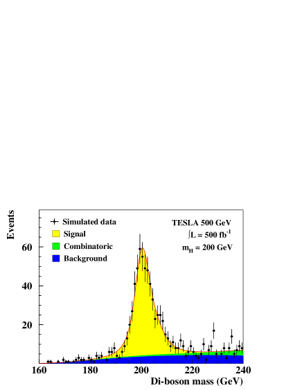
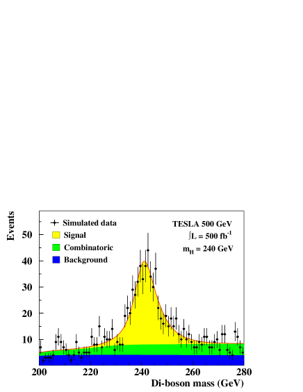
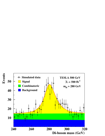
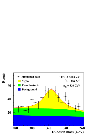
Figure 7: Di-boson mass spectra for the four Higgs masses under study. Everywhere, the higgs resonances (yellow) are clearly visible over physical (blue) and combinatorical (green) background for ${\cal\int\!\!L}=500\,\mathrm{fb}^{-1}$ of integrated luminosity at $\sqrt{s}=500\,\mathrm{GeV}$.

$m_{\mathrm{H}}$	$\frac{\Delta N}{N}$	$\frac{\Delta m}{m}$	$\frac{\Delta\Gamma}{\Gamma}$	$\frac{\Delta\mathrm{BR}_{\mathrm{H}\to\mathrm{W}\mathrm{W}}}{\mathrm{BR}_{\mathrm{H}\to\mathrm{W}\mathrm{W}}}$	$\frac{\Delta\mathrm{BR}_{\mathrm{H}\to\mathrm{Z}\mathrm{Z}}}{\mathrm{BR}_{\mathrm{H}\to\mathrm{Z}\mathrm{Z}}}$
$200\,\mathrm{GeV}$	$3.6\,\%$	$0.11\,\%$	$34.0\,\%$	$3.5\,\%$	$9.9\,\%$
$240\,\mathrm{GeV}$	$3.8\,\%$	$0.17\,\%$	$26.8\,\%$	$5.0\,\%$	$10.8\,\%$
$280\,\mathrm{GeV}$	$4.4\,\%$	$0.24\,\%$	$22.7\,\%$	$7.7\,\%$	$16.2\,\%$
$320\,\mathrm{GeV}$	$6.3\,\%$	$0.36\,\%$	$26.4\,\%$	$8.6\,\%$	$17.3\,\%$

Table 4: Resolutions for event rate $N$, Higgs mass $m_{\mathrm{H}}$ and Higgs width $\Gamma_{\mathrm{H}}$ as fitted to the di-boson mass spectrum. Also listed are results for the branching ratios $\mathrm{BR}_{\mathrm{H}\to\mathrm{W}\mathrm{W}}$ and $\mathrm{BR}_{\mathrm{H}\to\mathrm{Z}\mathrm{Z}}$ as described in Sec. 4. All numbers are mean values obtained with 100 independent signal samples corresponding to ${\cal\int\!\!L}=500\,\mathrm{fb}^{-1}$ at $\sqrt{s}=500\,\mathrm{GeV}$ each.

6 Summary and Conclusion

We present a method for measuring Higgs mass, width and event rate in a model independent fit from the reconstructed Higgs lineshape at TESLA. The method is restricted to Higgs bosons with widths as large as few $\mathrm{GeV}$. Otherwise, precision is spoiled by detector mass resolution which is in the same order. Assuming the Higgs decays to $\mathrm{W}$- and $\mathrm{Z}$-boson pairs only, determination of the corresponding branching ratios $\mathrm{BR}_{\mathrm{H}\to\mathrm{W}\mathrm{W}}$ and $\mathrm{BR}_{\mathrm{H}\to\mathrm{Z}\mathrm{Z}}$ is possible as well.

The selection is based on reconstructing $\mathrm{e^{+}e^{-}}\to\mathrm{H}\mathrm{Z}$ events with successive $\mathrm{H}\to\mathrm{W}\mathrm{W}/\mathrm{Z}\mathrm{Z}$ decays. Selecting final states with two charged leptons and four jets gives a good handle on background suppression and high event rates. Since identification of $\tau$-leptons is not modelled in the fast detector simulation used, only electrons and muons are considered.

Four jets are paired to two boson candidates by a 4C kinematic fit, two identified leptons form a third boson candidate. The Higgs resonance is reconstructed as di-boson mass. Higgs event rate, mass and width are extracted from the resonance lineshape in a model independent fit. The results of 100 independent MC experiments each corresponding to ${\cal\int\!\!L}=500\,\mathrm{fb}^{-1}$ of integrated luminosity lay within statistical expectation. Mean values of the precision achieved are listed in Tab. 4.

Main motivation for this study was to explore a direct method for measuring the total Higgs width $\Gamma_{\mathrm{H}}$. Before, this has only be studied for LHC experiments [13]. Results obtained in this study are comparable in precision for mass and width of the resonance. No LHC numbers are available for event rates, and branching ratio determination is impossible from the lineshape reconstruction.

Fig. 8 (left) compares the results obtained in this study on Higgs width and mass with previous TESLA studies on lower Higgs masses. For the Higgs width, the indirect determination via the Higgs coupling to $\mathrm{W}$-bosons, measured in the cross section of $\mathrm{W}\mathrm{W}$-fusion [7], is the most precise method studied so far. However, up to now only $\mathrm{H}\to\mathrm{b}\mathrm{\bar{\mathrm{b}}}$ decays have been investigated, so precision breaks down as does the branching ratio $\mathrm{BR}_{\mathrm{H}\to\mathrm{b}\mathrm{\bar{\mathrm{b}}}}$ at $m_{\mathrm{H}}\raisebox{-1.9919pt}{$\,\stackrel{{\scriptstyle>}}{{{\scriptstyle\sim}}}\,$}150\,\mathrm{GeV}$. On the other hand, precision for direct width determinations in the Higgs lineshape are limited by the narrow Higgs width below $m_{\mathrm{H}}\raisebox{-1.9919pt}{$\,\stackrel{{\scriptstyle<}}{{{\scriptstyle\sim}}}\,$}200\,\mathrm{GeV}$. The gap could be closed by indirect determinations with the analysis of $\mathrm{H}\to\mathrm{W}\mathrm{W}$ decays. The hope is, that combination of direct and indirect measurements significantly improves the precision on the Higgs width for high Higgs masses.

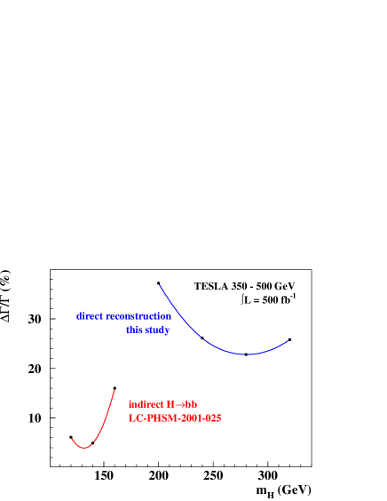
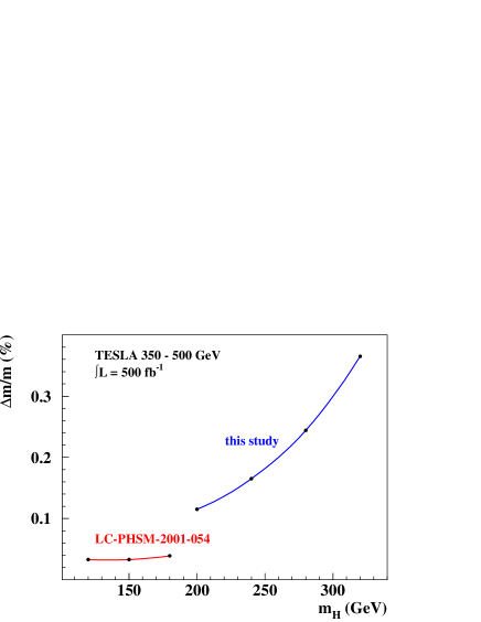
Figure 8: Precisions of Higgs width (left) and mass (right) measurements at TESLA. Results from former studies are shown in red, those of this simulation in blue.

Precisions of the direct method alone may be optimized as well. There are many ways to enhance signal event rates by considering more common final states. For instance, one could include $\mathrm{Z}\to\tau^{+}\tau^{-}$ or study $\mathrm{H}\mathrm{Z}\to\mathrm{q}\mathrm{q}\mathrm{q}\mathrm{q}\mathrm{q}\mathrm{q}$ and $\mathrm{H}\mathrm{Z}\to\mathrm{q}\mathrm{q}\mathrm{q}\mathrm{q}\ell\nu$ final states. But, the effects of larger background contributions and final state neutrinos need dedicated studies.

It is pointed out that this study is optimized for width determination. Results on mass, event rate and branching ratios are welcome spin-offs, but there might be other processes and methods still to be studied which are more appropriate. As an example, the precision on Higgs mass measurements of previous TESLA studies [14] is compared to results of this study in Fig. 8 (right). As can be seen, precision is about three times better in the dedicated study. The main reason, is selection of more common signal final states and thus higher statistics.

References

• [1] TESLA Technical Design Report, DESY-2001-011.
• [2] T. Abe et al. [American Linear Collider Working Group Collaboration], Linear collider physics resource book for Snowmass 2001, Proc. of the APS/DPF/DPB Summer Study on the Future of Particle Physics (Snowmass 2001), ed. N. Graf, SLAC-R-570.
• [3] K. Abe et al. [ACFA Linear Collider Working Group Collaboration], Particle physics experiments at JLC, arXiv:hep-ph/0109166.
• [4] P. Janot, Physics at LEP2, CERN 96-01, Vol.2, 309.
• [5] A. Djouadi, J. Kalinowski and M. Spira, HDECAY: a Program for Higgs Boson Decays in the Standard Model and its Supersymmetric Extensions, Comp. Phys. Comm. 108 (1998), 56.
• [6] G. Jikia, S. Söldner-Rembold, Light Higgs Production at a Photon Collider, Proceedings of the 7th International Workshop on High Energy Photon Colliders, Hamburg 2000, 133.
• [7] K. Desch, N. Meyer, Study of Higgs Boson Production through WW-fusion at TESLA, LC-PHSM-2001-025.
• [8] W. Kilian, WHiZard 1.22 - Manual, LC-TOOL-2001-039.
• [9] T. Sjostrand, L. Lonnblad and S. Mrenna, PYTHIA 6.2: Physics and manual, arXiv:hep-ph/0108264.
• [10] T. Ohl, CIRCE version 1.0: Beam spectra for simulating linear collider physics, Comp. Phys. Comm. 101 (1997), 269.
• [11] M. Pohl and H. J. Schreiber, SIMDET - Version 4: A parametric Monte Carlo for a TESLA detector, arXiv:hep-ex/0206009.
• [12] Y. Dokshitzer, J.Phys. G17, (1991), 1537;
N. Brown, W. J. Stirling, Phys. Lett. B252 (1990) 657;
S. Bethke et al., Nucl. Phys. B370 (1992) 310;
S. Catani et al., Phhys. Lett. B269 (1991),432;
N. Brown, W. J. Stirling, Z. Phys. C53 (1992) 629.
• [13] V. Drollinger and A. Sopczak, Eur. Phys. J. directC 3 (2001) N1.
• [14] P. Garcia-Abia, W. Lohmann and A. Raspereza, Measurement of the Higgs Boson Mass and Cross Section with a Linear $e^{+}e^{-}$ Collider, LC-PHSM-2001-054.