The Forward Backward asymmetries of $B\to X_{s}\tau^{+}\tau^{-}$ in the MSSM

Abstract:

The relatively clean theoretical probes of the Standard Model (SM), and the various theories beyond the SM, provided by radiative, semi-leptonic and (purely) leptonic decays of B-mesons have become increasingly important. Due to the large number of possible distributions in the semi-leptonic decays based on the quark level transition $b\to s\ell^{+}\ell^{-}$ (not just the branching ratio), these transitions have become very useful. A study of the Forward-Backward asymmetries for the inclusive decay ($B\to X_{s}\ell^{+}\ell^{-}$) is carried out in this paper. This study shall be performed in the SM and a minimal supersymmetric extension of the SM, namely the mSUGRA model.

1 Introduction

The recent flux of papers studying the various decay processes of B-mesons stands testimony to the great importance of this field in testing not only the parameters of the Standard Model (SM) but in constraining the parameters of its many possible extensions. In this vain processes of particular interest are the so called “rare” decays, these being transitions through loop levels only [1]. Of particular interest are the Flavour Changing Neutral Currents (FCNC) $b\to s(d)$. These rare decays are extremely sensitive to the masses and couplings of the virtual particles involved in this transition, and therefore provide the greatest hope of determining many of the SM’s (and its possible extensions) underlying structures. We therefore require a decay process which is both theoretically clean and experimentally realizable in the near future, such as $B\to X_{s}\gamma$ and $B\to X_{s}\ell^{+}\ell^{-}$. Of these two processes this paper shall focus on the inclusive decay mode, $B\to X_{s}\ell^{+}\ell^{-}$, for the reason that this decay mode is a far richer alternative to the radiative mode as here many distributions involving the final state lepton pair can be measured. In the inclusive decay channel ($B\to X_{s}\ell^{+}\ell^{-}$) observables such as Forward-Backward (FB) asymmetries and lepton polarization asymmetries, where one or both the leptons are polarized, have been extensively studied both within the SM and its various extensions [5, 2, 4].

Recently, it has been pointed out by Bensalem et al. [6] that one can construct the polarized FB asymmetries also (FB asymmetries when one or both the leptons are polarized). These new observables could provide a sufficiently large number of observables for a very strict testing of the SM and any new physics. These polarized FB asymmetries were studied in an exclusive decay mode ($B\to K\ell^{+}\ell^{-}$) both within the SM and the Minimal Supersymmetric SM (MSSM) [7], motivated by the vanishing unpolarized FB asymmetry for $B\to K\ell^{+}\ell^{-}$ within the SM [8, 9]. Based on the construction of doubly polarized observables by Bensalem et al. such observables were studied in the case of $B\to K^{*}\ell^{+}\ell^{-}$ [10] and in the inclusive mode [5]. In this work we will focus on the polarized FB asymmetries.

Lately there has been an increased interest in how the predictions of various observables will change in the two Higgs doublet model (2HDM) and Supersymmetric (SUSY) extensions of the SM. The primary reason for this is due to the increase in the number of particles in these theories, such as the Neutral Higgs Bosons (NHBs), and hence scalar and pseudo-scalar exchange operators are now included. Such operators give rise to many interesting new possibilities, like orders of enhancement in the branching ratio for purely leptonic decays ($B_{s,d}\to\ell^{+}\ell^{-}$) [11, 12] and non-vanishing values for unpolarized FB asymmetries in $B\to K(\pi)\ell^{+}\ell^{-}$ [7, 8, 9]. As the coupling of the NHBs to the leptons is proportional to the lepton mass [11, 14, 2, 12], the effects of these new particles is greater when the final state leptons are either $\mu$ or $\tau$. Therefore in this paper we will also consider the effect of the new scalar and pseudo-scalar operators which arise from a MSSM. The particular model to be employed shall be explained in more detail in section 4.

As such, this paper shall therefore be organized as follows: In section 2 we shall review the effective Hamiltonian and the matrix element for the process concerned, as derived from the quark level transition $b\to s\ell^{+}\ell^{-}$. Section 3 will then focus on the definitions and analytic results of the FB asymmetries. Finally, section 4 will contain our discussion and numerical analysis of the results.

2 Effective Hamiltonian

The effective Hamiltonian for the quark level transition $b\to s\ell^{+}\ell^{-}$, as first studied by Grinstein et al. (and later to NLO by Buras and Münz) [15], and represents the quark level process for the inclusive decay $B\to X_{s}\ell^{+}\ell^{-}$, under consideration (where we shall use descriptions as penned in references [11, 14, 2]);

$${\cal H}_{eff}=\frac{4G_{F}}{\sqrt{2}}V_{tb}V^{*}_{ts}\left(\sum_{i=1}^{10}C_{i}O_{i}+\sum_{i=1}^{10}C_{Q_{i}}Q_{i}\right)$$ (1)

where the $O_{i}$ operators are the current-current (i=1, 2), penguin (i=3,…,6), magnetic penguin (i=7,8) and semi-leptonic (i = 9,10) operators with the $C_{i}$ corresponding to the standard Wilson coefficients. The additional operators $Q_{i}$ (i = 1,…,10) and their Wilson coefficients ($C_{Q_{i}}$) are related to the additional particles of the MSSM under consideration.

Using the above effective Hamiltonian, and neglecting the s-quark mass, the matrix element for the quark level transition $b\to s\ell^{+}\ell^{-}$ is;

$${\cal M} = \frac{\alpha G_{F}}{\sqrt{2}\pi}V_{tb}V^{*}_{ts}\Bigg{\{}-2C_{7}^{eff}\frac{m_{b}}{q^{2}}(\bar{s}i\sigma_{\mu\nu}q^{\nu}P_{R}b)(\bar{\ell}\gamma^{\mu}\ell)+C_{9}^{eff}(\bar{s}\gamma_{\mu}P_{L}b)(\bar{\ell}\gamma^{\mu}\ell)$$ (2)

$$\hskip 56.9055pt+C_{10}(\bar{s}\gamma_{\mu}P_{L}b)(\bar{\ell}\gamma^{\mu}\gamma_{5}\ell)+C_{Q_{1}}(\bar{s}P_{R}b)(\bar{\ell}\ell)+C_{Q_{2}}(\bar{s}P_{R}b)(\bar{\ell}\gamma_{5}\ell)\Bigg{\}}.$$

In this expression $q$ represents the momentum transferred to the lepton pair, given as $q=p_{+}+p_{-}$, where $p_{+}$ and $p_{-}$ are the momentas of the $\ell^{+}$ and $\ell^{-}$ particles respectively. Note also that the CKM factors have been denoted $V_{tb}V^{*}_{ts}$ above, and that $P_{L,R}=(1\mp\gamma_{5})/2$.

In this paper we will also include the long range effects which arise from the four quark operators $\langle\ell^{+}\ell^{-}s|O_{i}|b\rangle$ for $i=1,\dots,6$. This shall be done by absorbing them into the description of the Wilson coefficients; a prescription which has been used in many earlier works, see references [4, 17]. These long distance effects typically arise from $c\bar{c}$ contributions, and are taken into account by adding a term to the $C_{9}^{eff}$ coefficient;

$$C_{9}^{res}\propto\kappa\sum_{V=\psi}\frac{\hat{m}_{V}Br(V\to\ell^{-}\ell^{+})\hat{\Gamma}^{V}_{total}}{\hat{s}-\hat{m}_{V}^{2}+i\hat{m}_{V}\hat{\Gamma}^{V}_{total}}$$ (3)

where we have used the same symbols and notation as in Krüger and Sehgal [4]. In the above equation the phenomenological factor $\kappa$ is introduced to predict the correct branching ratio of $Br(B\to J/\Psi X_{s}\to X_{s}\ell^{+}\ell^{-})$. For our numerical analysis we will choose $\kappa$ to have a value of 2.3.

Using the expression of matrix element in equation (2) we obtain the expression for the differential decay rate as;

$$\frac{d\Gamma}{d\hat{s}}=\frac{G_{F}m_{b}^{5}}{192\pi^{3}}\frac{\alpha^{2}}{4\pi^{2}}|V_{tb}V_{ts}^{*}|^{2}(1-\hat{s})^{2}\sqrt{1-\frac{4\hat{m}_{\ell}^{2}}{\hat{s}}}\bigtriangleup$$ (4)

with

$$\bigtriangleup = 4\frac{(2+\hat{s})}{\hat{s}}\left(1+\frac{2\hat{m}_{\ell}^{2}}{\hat{s}}\right)|C_{7}^{eff}|^{2}+(1+2\hat{s})\left(1+\frac{2\hat{m}_{\ell}^{2}}{\hat{s}}\right)|C_{9}^{eff}|^{2}$$ (5)

$$+(1-8\hat{m}_{\ell}^{2}+2\hat{s}+\frac{2\hat{m}_{\ell}^{2}}{\hat{s}})|C_{10}|^{2}+{3\over 2}(-4\hat{m}_{\ell}^{2}+\hat{s})|C_{Q_{1}}|^{2}+{3\over 2}\hat{s}|C_{Q_{2}}|^{2}$$

$$+12(1+\frac{2\hat{m}_{\ell}^{2}}{\hat{s}})Re(C_{9}^{eff*}C_{7}^{eff})+6\hat{m}_{\ell}Re(C_{10}^{*}C_{Q_{2}}).$$

Using this expression of the invariant mass spectrum (including the scalar exchange effects) we will now analyze the various FB asymmetries in the next section.

3 Polarized FB asymmetries

As was mentioned in the introduction, the additional intricacies of the $b\to s\ell^{+}\ell^{-}$ quark level transition requires many more experimental observables in processes such as $B\to X_{s}\ell^{+}\ell^{-}$ in order to constrain all the parameters of a particular MSSM. With this in mind we shall now define the differential FB asymmetry as [17];

$$\overline{{\mathcal{A}}}(\hat{s})=\int_{0}^{1}\frac{d^{2}\Gamma}{d\hat{s}dz}dz-\int_{-1}^{0}\frac{d^{2}\Gamma}{d\hat{s}dz}dz.$$ (6)

If we do not sum over the spins of the outgoing leptons then the FB asymmetry will, in general, be a function of the spins of the final state leptons; and can be defined as

$$\overline{{\mathcal{A}}}(s^{-},s^{+},\hat{s})=\int_{0}^{1}\frac{d^{2}\Gamma(s^{-},s^{+})}{d\hat{s}dz}dz-\int_{-1}^{0}\frac{d^{2}\Gamma(s^{-},s^{+})}{d\hat{s}dz}dz.$$ (7)

As our eventual aim is to derive expressions to be searched for in experiments it is convenient to use the normalized FB asymmetry. Normalizing the above (equation 7) definition by dividing by the total decay rate we get;

$${\mathcal{A}}(s^{-},s^{+},\hat{s})=\frac{\overline{\mathcal{A}}(s^{-},s^{+},\hat{s})}{d\Gamma/d\hat{s}}.$$ (8)

We can split the FB asymmetries into their various polarization components and we will do this in analogy to the prescription given in Bensalem et al. [6];

$${\mathcal{A}}(s^{-},s^{+})={\mathcal{A}}+{\mathcal{A}}_{i}s_{i}^{-}+{\mathcal{A}}_{i}s_{i}^{+}{\mathcal{A}}_{ij}s_{i}^{+}s_{j}^{-}$$ (9)

where $i,j=L,T,N$ are the longitudinal, transverse and normal components of the polarization. Therefore, from equation (9) we can write the single polarized FB asymmetry as;

$${\mathcal{A}}_{i}^{-}={\mathcal{A}}(s^{-}=i,s^{+}=j)+{\mathcal{A}}(s^{-}=i,s^{+}=-j)-{\mathcal{A}}(s^{-}=-i,s^{+}=j)-{\mathcal{A}}(s^{-}=-i,s^{+}=-j)$$

(10)

$${\mathcal{A}}_{i}^{+}={\mathcal{A}}(s^{-}=j,s^{+}=i)+{\mathcal{A}}(s^{-}=-j,s^{+}=i)-{\mathcal{A}}(s^{-}=j,s^{+}=-i)-{\mathcal{A}}(s^{-}=-j,s^{+}=-i),$$

(11)

and the double polarized FB asymmetry as;

$${\mathcal{A}}_{ij}={\mathcal{A}}(s^{-}=i,s^{+}=j)-{\mathcal{A}}(s^{-}=i,s^{+}=-j)-{\mathcal{A}}(s^{-}=-i,s^{+}=j)+{\mathcal{A}}(s^{-}=-i,s^{+}=-j).$$ (12)

Using the expression of the matrix element as given in equation (2) we can get the expression of unpolarized FB asymmetry;

$${\mathcal{A}} = \frac{3}{\bigtriangleup}\sqrt{1-\frac{4\hat{m}_{\ell}^{2}}{\hat{s}}}$$ (13)

$$\times\left[2Re(C_{7}^{eff}C_{10})+\hat{s}Re(C_{9}^{eff}C_{10})+\hat{m}_{\ell}\left\{Re(C_{9}^{eff*}C_{Q_{1}})+Re(C_{7}^{eff*}C_{Q_{1}})\right\}\right]$$

The analytical results of the polarized FB asymmetries are then;

$${\mathcal{A}}^{-}_{L} = \frac{1}{\bigtriangleup}\left[6\frac{1}{\hat{s}}|C_{7}^{eff}|^{2}+{3\over 2}\hat{s}|C_{9}^{eff}|^{2}+{3\over 2}\hat{s}\left(1-\frac{4\hat{m}_{\ell}^{2}}{\hat{s}}\right)|C_{10}|^{2}+6Re(C_{7}^{eff*}C_{9}^{eff})\right.$$ (14)

$$\hskip 28.45274pt-12\frac{\hat{m}_{\ell}^{2}}{\hat{s}}Re(C_{7}^{eff*}C_{10})-6\hat{m}_{\ell}Re(C_{7}^{eff*}C_{Q_{2}})-6\frac{\hat{m}_{\ell}^{2}}{\hat{s}}Re(C_{9}^{eff*}C_{10})$$

$$\hskip 28.45274pt+3\hat{m}_{\ell}Re(C_{9}^{eff*}C_{Q_{2}})\Bigg{]}$$

$${\mathcal{A}}^{-}_{N} = 0$$ (15)

$${\mathcal{A}}^{-}_{T} = \frac{2}{\bigtriangleup}\frac{(1-\hat{s})\hat{m}_{\ell}}{\sqrt{\hat{s}}}\sqrt{1-\frac{4\hat{m}_{\ell}^{2}}{\hat{s}}}Re(C_{9}^{eff*}C_{10})$$ (16)

$${\mathcal{A}}^{+}_{L} = -\frac{1}{\bigtriangleup}\left[6\frac{1}{\hat{s}}|C_{7}^{eff}|^{2}+{3\over 2}\hat{s}|C_{9}^{eff}|^{2}+{3\over 2}\hat{s}\left(1-\frac{4\hat{m}_{\ell}^{2}}{\hat{s}}\right)|C_{10}|^{2}+6Re(C_{7}^{eff*}C_{9}^{eff})\right.$$ (17)

$$\hskip 28.45274pt+12\frac{\hat{m}_{\ell}^{2}}{\hat{s}}Re(C_{7}^{eff*}C_{10})+6\hat{m}_{\ell}Re(C_{7}^{eff*}C_{Q_{2}})+6\frac{\hat{m}_{\ell}^{2}}{\hat{s}}Re(C_{9}^{eff*}C_{10})$$

$$\hskip 28.45274pt+3\hat{m}_{\ell}Re(C_{9}^{eff*}C_{Q_{2}})\Bigg{]}$$

$${\mathcal{A}}^{+}_{N} = 0$$ (18)

$${\mathcal{A}}^{+}_{T} = -\frac{2}{\bigtriangleup}\frac{(1-\hat{s})\hat{m}_{\ell}}{\sqrt{\hat{s}}}\sqrt{1-\frac{4\hat{m}_{\ell}^{2}}{\hat{s}}}Re(C_{9}^{eff*}C_{10})$$ (19)

$${\mathcal{A}}_{LL} = \frac{3}{\bigtriangleup}\sqrt{1-\frac{4\hat{m}_{\ell}^{2}}{\hat{s}}}$$

$$\hskip 19.91684pt\times\left[-2Re(C_{7}^{eff}C_{10})-\hat{s}Re(C_{9}^{eff}C_{10})+\hat{m}_{\ell}\left\{Re(C_{9}^{eff*}C_{Q_{1}})+Re(C_{7}^{eff*}C_{Q_{1}})\right\}\right]$$

$${\mathcal{A}}_{LN} = -\frac{2}{\bigtriangleup}\frac{(1-\hat{s})\hat{m}_{\ell}}{\sqrt{\hat{s}}}\sqrt{1-\frac{4\hat{m}_{\ell}^{2}}{\hat{s}}}Im(C_{10}^{*}C_{9}^{eff})$$ (21)

$${\mathcal{A}}_{LT} = \frac{2}{\bigtriangleup}\frac{\hat{m}_{\ell}}{\sqrt{\hat{s}}}\left(-12\frac{|C_{7}^{eff}|^{2}}{\hat{s}}+|C_{9}^{eff}|^{2}\right)$$ (22)

$${\mathcal{A}}_{NL} = -{\mathcal{A}}_{LN}$$ (23)

$${\mathcal{A}}_{NN} = -\frac{3}{\bigtriangleup}\hat{m}_{\ell}\left(2Re(C_{7}^{eff*}C_{Q_{1}})+Re(C_{9}^{eff*}C_{Q_{1}})\right)\sqrt{1-\frac{4\hat{m}_{\ell}^{2}}{\hat{s}}}$$ (24)

$${\mathcal{A}}_{NT} = \frac{6}{\bigtriangleup}\hat{m}_{\ell}\left(2\frac{\hat{m}_{\ell}}{\hat{s}}Im(C_{10}^{*}C_{7}^{eff})-Im(C_{7}^{eff*}C_{Q_{2}})+\frac{\hat{m}_{\ell}}{\hat{s}}Im(C_{10}^{*}C_{9}^{eff})\right)$$ (25)

$${\mathcal{A}}_{TL} = -{\mathcal{A}}_{LT}$$ (26)

$${\mathcal{A}}_{TN} = {\mathcal{A}}_{NT}$$ (27)

$${\mathcal{A}}_{TT} = -{\mathcal{A}}_{NN}$$ (28)

where $\bigtriangleup$ is given in equation (5). We will discuss the above obtained expressions of the various FB asymmetries and present our numerical analysis of the same in the next section.

4 Numerical analysis and Conclusions

As it is experimentally more useful we shall present our results in the form of average values. Though, as is well known [27], we have modelled the inclusive decay $B\to X_{s}\ell^{+}\ell^{-}$ from a quark level transition $b\to s\ell^{+}\ell^{-}$ using the Heavy Quark Expansion (HQE) in $(1/m_{b})$, where in this expansion we have used the first term of this expansion. However, this expansion breaks down when $\hat{s}\to 1$. In fact for higher values of $\hat{s}$ one should consider the non-perturbative $(1/m_{b}^{2})$ corrections as well [27]. As was also shown in [27] it is difficult to estimate these non-perturbative corrections for $\hat{s}\gtrsim 0.8$ . For our analysis we have placed a cutoff on the upper limit of $\hat{s}$. The averaging procedure which we will be using is defined as:

$$\langle{\mathcal{A}}\rangle\equiv\frac{\displaystyle{\int_{(3.646+0.02)^{2}/m_{b}^{2}}^{0.8}}{\mathcal{A}}\frac{d\Gamma}{d\hat{s}}d\hat{s}}{\displaystyle{\int_{(3.646+0.02)^{2}/m_{b}^{2}}^{0.8}}\frac{d\Gamma}{d\hat{s}}d\hat{s}},$$ (29)

that is, in the calculation of our averages we have taken the lower limit of integration to be above the first resonance. Note that we have used the input parameters presented in appendix A. The results of table 1, these being our SM predictions of the integrated observables, will of course be altered when considering a MSSM.

Figure 1: The variation of the branching ratio of $B\to X_{s}\tau^{+}\tau^{-}$ with $tan\beta$ in the mSUGRA model. Other model parameters are: $m_{1/2}=450$GeV, $A=200$GeV and the sign of $\mu$ will be taken to be positive for all our numerical analysis

Br($B\to X_{s}\tau^{+}\tau^{-}$)	${\mathcal{A}}$	${\mathcal{A}}^{-}_{L}$	${\mathcal{A}}^{-}_{T}$	${\mathcal{A}}_{LL}$	${\mathcal{A}}_{LN}$	${\mathcal{A}}_{LT}$	${\mathcal{A}}_{NN}$	${\mathcal{A}}_{NT}$
$1.8\times 10^{-7}$	- 0.176	0.455	-0.029	0.176	-0.0084	0.063	0	-0.083

Table 1: Our SM predictions of the integrated observables

We have also performed the numerical analysis of the SUSY effects on various observables, presented in the previous section, for the inclusive mode ($B\to X_{s}\tau^{+}\tau^{-}$). If we assume that SUSY exists, then the MSSM is the simplest SUSY extension of the SM. However, the MSSM has a large number of parameters, which limits its practical usage for phenomenological studies. There are many models which reduce the vast MSSM parameter space to a manageable set of parameters. These include Dilaton, Moduli, mSUGRA (minimal Supergravity), rSUGRA (relaxed SUGRA), CMSSM (constraint MSSM) etc. All of these models have their own characteristics. The basic feature of all these unified models is that they assume some unification of the parameters at a higher scale (usually at the GUT scale). In our numerical analysis we have used one of the more popular models, minimal Supergravity or mSUGRA.

Figure 2: $A_{NN}$ variation with the invariant mass of the dileptons, $\hat{s}$, in the mSUGRA model. The other model parameters are: $m_{0}=400$GeV, $m_{1/2}=500$GeV, $A=0$.

In the mSUGRA model one assumes the universality of masses and coupling constants at the GUT scale. The mSUGRA framework has five independent parameters namely, $m_{0}$ (the unified mass of all the scalars), $m_{1/2}$ (the unified mass of all the gauginos), $A$ (the unified trilinear coupling constants), $tan\beta$ (the ratio of vacuum expectation values of the two Higgs doublets). Using these unified parameters the renormalization group (RG) equations of all the parameters are evolved from the GUT scale to the electroweak scale and then at the electroweak scale one imposes the condition of electroweak symmetry breaking (EWSB). Imposition of EWSB fixes the magnitude of the parameter $\mu$ , but the sign of $\mu$ still remains arbitrary. As such the $sgn(\mu)$ is taken to be another parameter, which makes for five parameters (out of these five, four are continuous parameters with the of $sgn(\mu)$ being discrete, that is $\pm 1$).

Figure 3: Plots of various integrated FB asymmetries with the branching ratio of the inclusive mode ($B\to X_{s}\tau^{+}\tau^{-}$) in the mSUGRA model. The mSUGRA parameters are: $m_{0}=500$GeV, $m_{1/2}=450$GeV, $A=0$. In these plots we have varied $tan\beta$ in the range $25\leq tan\beta\leq 50$.

Furthermore, we have worked in the high $tan\beta$ region of the mSUGRA parameter space. This was done as it is only in this region that the contributions of the Neutral Higgs Bosons (NHBs) become significant [11, 14, 2, 10, 12]. The parameter space of mSUGRA has been constrained by the experimental observation of $B\to X_{s}\gamma$ [19]. For our numerical analysis we will use a more generous bound [19]:

$$2\times 10^{-4}<Br(B\to X_{s}\gamma)<4.5\times 10^{-4}$$

which is in agreement with CLEO [20], ALEPH [21], BELLE [23] and BaBar [24] results. We have checked that the qualitative nature of our results doesn’t change even if we use a much stronger bound on the branching ratio of $B\to X_{s}\gamma$. As has already been mentioned in many earlier works [11] it is the purely dileptonic decay, $B_{s}\to\mu^{+}\mu^{-}$ which is most affected by the introduction of the new set of operators. Therefore this decay would be one of the most promising modes to search for signatures of these new operators. The SM prediction of this mode is $\sim 10^{-9}$, which would be enhanced by many orders by these new operators. This process ($B_{s}\to\mu^{+}\mu^{-}$) has not yet been observed in B-factories but CDF has given an upper limit on this branching ratio [25]. For our numerical analysis we have considered only that region of the mSUGRA parameter space which complies with the new CDF Run II bound $Br(B_{s}\to\mu^{+}\mu^{-})<9.5\times 10^{-7}$ [25] .

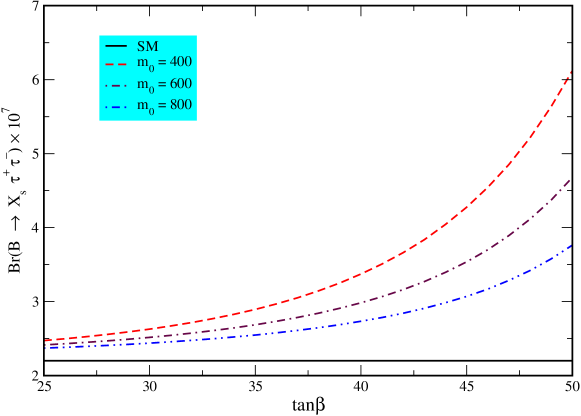
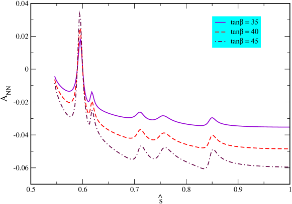
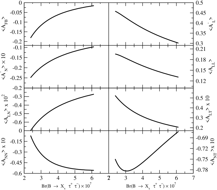
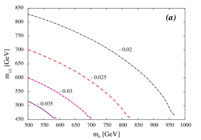
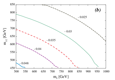
In Figure 1 we have shown the plots of the branching ratio of the process concerned as a function of $tan\beta$ for various values of $m_{0}$. In Figure 2 we have shown the variation of the ${\mathcal{A}}_{NN}$ with the invariant mass of the dileptons ($\hat{s}$) for various values of $tan\beta$. As can be seen from the expression of ${\mathcal{A}}_{NN}$ given in equation (24) (and also given in Table 1) the asymmetry vanishes within the SM, as within the SM the scalar and pseudo-scalar operators are negligibly small ($\sim m_{\ell}m_{b}/m_{W}^{2}$). Therefore any observation of this asymmetry can be considered as a signal of new physics. In Figure 3 we have shown the values of various integrated FB asymmetries as a function of the branching ratio. In Figure 4 we have shown the contour plots of ${\mathcal{A}}_{NN}$ in the $[m_{0},m_{1/2}]$ plane for two different values of $tan\beta$.

As has been mentioned in many earlier works [11, 14, 2, 10, 12], the effect of the scalar (and pseudo-scalar) operators crucially depends on $tan\beta$ and the mass of the Higgs. One could have used some relaxed kind of SUGRA framework also. By relaxed we mean relaxing the universality of the masses and coupling constants. Here we can relax the conditions of universality of scalar and/or gaugino masses. In the literature these models have been termed as rSUGRA (or relaxed SUGRA models) [18]. In these situations one can have sufficiently low allowed values of the Higgs mass for large $tan\beta$. In such situations the numerical values of the Wilson coefficients accompanying the scalar and pseudo-scalar operators could be high, and hence their effects on observables could be more profound. Similarly one could have used CMSSM models, where even the condition of correct electroweak symmetry breaking is relaxed. In these models one can have a very large variation in the Wilson coefficients $C_{Q_{1}}$ and $C_{Q_{2}}$. However, in this work we have confined ourselves to the mSUGRA model.

Figure 4: Contour plots of various values of averaged $<{\mathcal{A}}_{NN}>$ (as given in plots) in the $[m_{0},m_{1/2}]$ plane for the mSUGRA model with $A=0$ and (a) $tan\beta=40$, (b) $tan\beta=45$.

So far no experimental search for the inclusive decay mode $B\to X_{s}\tau^{+}\tau^{-}$ has been carried out. Experimentally this decay can be searched for by observing the $\mu$ produced from the $\tau$ via the $\tau\to\mu\nu\bar{\nu}$ process, but the muons produced in this cascade decay would be soft ones (so to be observed one has to observe muon pairs at low invariant mass). But there was an upper bound put on the branching ratio of this mode ($B\to X_{s}\tau^{+}\tau^{-}$) by Grossman et al. [28] which was:

$$Br(B\to X_{s}\tau^{+}\tau^{-})<5\%.$$

As the $\tau$ detection efficiency is low, such that at the SM level this decay mode might remain out of reach of the present generation B-factories (like BaBar, BELLE etc.), it has been well emphasized in many earlier works [3, 28, 14] that this decay can be enhanced by a couple of orders in magnitude in the presence of new physics and hence could be very useful in putting bounds on new physics models.

To summarize the major conclusions of our numerical analysis:

1. Almost all the polarized asymmetries show a large variation from their respective SM values over a large parameter space at large $tan\beta$.

2. The SM relationship that the magnitude of ${\mathcal{A}}_{LL}$ is the same as ${\mathcal{A}}$ is violated in the presence of new operators.

3. The observation of a non-vanishing value for ${\mathcal{A}}_{NN}$ could be treated clearly as a signal of new physics.

These polarized FB asymmetries also provide us with much needed observables, which could aid in the testing of the effective Hamiltonian’s structure; especially the scalar and pseudo-scalar parts as can be see from the expression for ${\mathcal{A}}_{NN}$ which is proportional to $C_{Q_{1}}$ and hence vanishes within the SM.

Appendix A Input parameters

$m_{b}~{}=~{}4.8$ GeV  ,  $m_{c}~{}=~{}1.4$ GeV

$m_{\tau}~{}=~{}1.77$ GeV  ,  $m_{w}~{}=~{}80.4$ GeV  ,

$m_{z}~{}=~{}91.19$ GeV  ,  $V_{tb}V^{*}_{ts}=0.0385$ ,

$\alpha={1\over 129}$  ,  $G_{F}=1.17\times 10^{-5}~{}{\rm GeV}^{-2}$

References

- [1] G. Buchalla, A. J. Buras and M. E. Lautenbacher, Rev. Mod. Phys. 68 (1996) 1125 [hep-ph/9512380].
- [2] S. Rai Choudhury, A. Gupta and N. Gaur, Phys. Rev. D 60 (1999) 115004 [hep-ph/9902355]; S. Fukae, C. S. Kim and T. Yoshikawa, Phys. Rev. D 61 (2000) 074015 [hep-ph/9908229];
- [3] D. Guetta and E. Nardi, Phys. Rev. D 58 (1998) 012001 [hep-ph/9707371].
- [4] F. Krüger and L. M. Sehgal, Phys. Lett. B 380 (1996) 199 [hep-ph/9603237]; J. L. Hewett, Phys. Rev. D 53 (1996) 4964 [hep-ph/9506289].
- [5] N. Gaur, hep-ph/0305242.
- [6] W. Bensalem, D. London, N. Sinha and R. Sinha, Phys. Rev. D 67 (2003) 034007 [hep-ph/0209228].
- [7] S. R. Choudhury, A. S. Cornell, N. Gaur and G. C. Joshi, hep-ph/0307276.
- [8] C. Bobeth, T. Ewerth, F. Kruger and J. Urban, Phys. Rev. D 64 (2001) 074014 [hep-ph/0104284]; D. A. Demir, K. A. Oliev and M. B. Voloshin Phys. Rev. D 66 (2002) 034015 [hep-ph/0204119].
- [9] E. O. Iltan , Int. J. Mod. Phys. D A 14 (1999) 4365 [hep-ph/9807256] ; T. M. Aliev and M. Savci , Phys. Rev. D 60 (1999) 014005 [hep-ph/9812272] ; S. R. Choudhury and N. Gaur, Phys. Rev. D 66 (2002) 094015 [hep-ph/0206128] ; G. Erkol and G. Turan, J. High Energy Phys. 0202 (2002) 015 [hep-ph/0201055].
- [10] S. R. Choudhury, N. Gaur, A. S. Cornell and G. C. Joshi, accepted for publication in Phys. Rev. D [hep-ph/0304084].
- [11] S. R. Choudhury and N. Gaur, Phys. Lett. B 451 (1999) 86 [hep-ph/9810307]; P. H. Chankowski and L. Slawianowska, Phys. Rev. D 63 (2001) 054012 [hep-ph/0008046]; A. J. Buas, P. H. Chankowski, J. Rosiek and L. Slawianowska, Nucl. Phys. B 659 (2003) 3 [hep-ph/0210145]; A. J. Buras, P. H. Chankowski, J. Rosiek and L. Slawianowska, Phys. Lett. B 546 (2002) 96 [hep-ph/0207241]; J. K. Mizukoshi, X. Tata and Y. Wang, Phys. Rev. D 66 (2002) 115003 [hep-ph/0208078]; T. Ibrahim and P. Nath, Phys. Rev. D 67 (2003) 016005 [hep-ph/0208142]; C. S. Huang and W. Liao, Phys. Lett. B 538 (2002) 301 [hep-ph/0201121]; S. Baek, P. Ko and W. Y. Song, Phys. Rev. Lett. 89 (2002) 271801 [hep-ph/0205259]; A. Dedes and A. Pilaftsis, Phys. Rev. D 67 (2003) 015012 [hep-ph/0209306]. C. S. Huang, W. Liao, Q. S. Yan and S. H. Zhu, Phys. Rev. D 63 (2001) 114021 [Erratum-ibid. D 64, 059902 (2001)] [hep-ph/0006250]; C. S. Huang and X. H. Wu, Nucl. Phys. B 657, 304 (2003) [hep-ph/0212220].
- [12] W. Skiba and J. Kalinowski, Nucl. Phys. B 404 (1993) 3; H. E. Logan and U. Nierste, Nucl. Phys. B 586 (2000) 39 [hep-ph/0004139];
- [13] P. L. Cho, M. Misiak and D. Wyler, Phys. Rev. D 54 (1996) 3329 [hep-ph/9601360]; J. L. Hewett and J. D. Wells, Phys. Rev. D 55 (1997) 5549 [hep-ph/9610323].
- [14] Z. Xiong and J. M. Yang, Nucl. Phys. B 628 (2002) 193 [hep-ph/0105260]; C. Bobeth, A. J. Buras, F. Kruger and J. Urban, Nucl. Phys. B 630 (2002) 87 [hep-ph/0112305]; C. Huang, W. Liao and Q. Yan, Phys. Rev. D 59 (1999) 011701 [hep-ph/9803460].
- [15] B. Grinstein, M. J. Savage and M. B. Wise, Nucl. Phys. B 319 (1989) 271 . A. J. Buras and M. Münz, Phys. Rev. D 52 (1995) 186 [hep-ph/9501281].
- [16] A. Ghinculov, T. Hurth, G. Isidori and Y. P. Yao, Nucl. Phys. 116 (Proc. Suppl.) (2003) 284 [hep-ph/0211197]; A. Ghinculov, T. Hurth, G. Isidori and Y. P. Yao, Nucl. Phys. B 648 (2003) 254 [hep-ph/0208088] ; P. Gambino, M. Gorbahn and U. Haisch, hep-ph/0306079 ; C. Bobeth, M. Misiak and J. Urban, Nucl. Phys. B 574 (2000) 291 [hep-ph/9910220] ; H. H. Asatrian, H. M. Asatrian, C. Greub and M. Walker, Phys. Lett. B 507 (2001) 162 [hep-ph/0103087] ; H. H. Asatryan, H. M. Asatrian, C. Greub and M. Walker, Phys. Rev. D 65 (2002) 074004 [hep-ph/0109140].
- [17] A. Ali, T. Mannel and T. Morozumi, Phys. Lett. B 273 (1991) 505 ; C. S. Lim, T. Morozumi and A. I. Sanda, Phys. Lett. B 218 (1989) 343 ; N. G. Deshpande, J. Trampetic and K. Panose, Phys. Rev. D 39 (1989) 1461 ; P. J. O’Donnell and H. K. Tung, Phys. Rev. D 43 (1991) 2067 .
- [18] T. Goto, Y. Okada, Y. Shimizu and M. Tanaka, Phys. Rev. D 55 (1997) 4273 [hep-ph/9609512]; T. Goto, Y. Okada and Y. Shimizu, Phys. Rev. D 58 (1998) 094006 [hep-ph/9804294]; J. R. Ellis, K. A. Olive and Y. Santoso, Phys. Lett. B 539 (2002) 107 [hep-ph/0204192] .
- [19] B Physics at Tevatron : Run II & Beyond , K. Anikeev et al. hep-ph/0201071 ;
- [20] CLEO collaboration, T.E.Coan et al. Phys. Rev. Lett. 84 (2000) 5283 [hep-ex/9908022] .
- [21] ALEPH Collaboration, R.Barate et al. Phys. Lett. B 429 (1998) 169 .
- [22] H. P. Nilles, Phys. Rept. 110 (1984) 1 .
- [23] K. Abe et al. [Belle Collaboration], Phys. Lett. B 511 (2001) 151 [hep-ex/0103042].
- [24] B. Aubert et al. [BABAR Collaboration], hep-ex/0207074 ; B. Aubert et al. [BaBar Collaboration], hep-ex/0207076.
- [25] Talk given by M. Nakao at Lepton Photon 2003, XXI Symposium on Lepton and Photon interactions at High Energies, Fermilab
- [26] F. Abe et al. [CDF Collaboration], Phys. Rev. D 57 (1998) 3811.
- [27] A. Ali, G. Hiller, L. T. Handoko and T. Morozumi, Phys. Rev. D 55 (1997) 4105 [hep-ph/9609449] ; G. Buchalla and G. Isidori, Nucl. Phys. B 525 (1998) 333 [hep-ph/9801456] ; A. V. Manohar and M. B. Wise, Phys. Rev. D 49 (1994) 1310 [hep-ph/9308246].
- [28] Y. Grossman, Z. Ligeti and E. Nardi, Phys. Rev. D 55 (1997) 2768 [hep-ph/9607473].