$e^{+}e^{-}\to H^{+}e^{-}\bar{\nu}$ in the two-Higgs-doublet model

Abstract

We calculate the cross section for $e^{+}e^{-}\to H^{+}e^{-}\bar{\nu}$ in the two-Higgs-doublet model from one-loop diagrams involving top and bottom quarks. This process offers the possibility of producing the charged Higgs boson at the $e^{+}e^{-}$ collider when its mass is more than half the center-of-mass energy, so that charged Higgs pair production is kinematically forbidden. The cross section receives contributions from both $s$-channel and $t$-channel processes; the $s$-channel contribution dominates for center-of-mass energies of 1 TeV and below. About 80% of the $s$-channel contribution comes from the resonant process $e^{+}e^{-}\to H^{+}W^{-}$, with $W^{-}\to e^{-}\bar{\nu}$. The cross section is generally small, below 0.01 fb for $\tan\beta>2$, and falls with increasing $\tan\beta$.

I Introduction

The Higgs mechanism provides an elegant way to explain electroweak symmetry breaking and the origin of the masses of the Standard Model fermions. In the Standard Model with a single Higgs doublet, however, the mass of the Higgs boson (and, therefore, the energy scale of electroweak symmetry breaking) is quadratically sensitive to physics at high energy scales via radiative corrections. This sensitivity leads to a fine-tuning problem between the electroweak scale and the cutoff (grand unification or Planck) scale.

Models that address the fine-tuning problem often enlarge the Higgs sector. For example, the Higgs sectors of the Minimal Supersymmetric Standard Model (MSSM) HaberKane , topcolor-assisted technicolor TC2 , and some of the “little Higgs” models LH2HDM contain two Higgs doublets with electroweak-scale masses. This enlargement of the Higgs sector leads to the presence of a charged Higgs boson in the physical spectrum, in addition to extra neutral states. Observation of these extra Higgs bosons and the measurement of their properties is a central goal in searches for physics beyond the Standard Model. In this paper we focus on the charged Higgs boson, $H^{\pm}$.

Unlike the CP-even Higgs sector, in which at least one of the CP-even Higgs bosons is guaranteed to be detected at future colliders lhcATLAS ; lhcCMS ; perini ; Espinosa:1998xj , the discovery of the heavy charged Higgs boson poses a special experimental challenge. Studies of charged Higgs boson production at present and future colliders are generally done in the context of the MSSM, or more generically, in a general two Higgs doublet model (2HDM). Searches for $H^{+}H^{-}$ pair production at the CERN LEP-2 collider only set a lower bound on the charged Higgs mass of $m_{H^{\pm}}>78.6$ GeV LEPHpm . At Run II of the Fermilab Tevatron, now in progress, the charged Higgs boson could be discovered in top quark decays if $m_{H^{\pm}}\mathrel{\raise 1.29167pt\hbox{$<$\kern-7.5pt\lower 4.30554pt\hbox{$\sim$}}}m_{t}$ and if $\tan\beta$ (the ratio of vacuum expectation values of the two Higgs doublets) is large topdecays . No sensitivity is expected in direct production unless QCD and supersymmetry (SUSY) effects conspire to enhance the cross section BelyaevHpm .

The difficulty of discovering a heavy charged Higgs boson comes from the fact that there are no tree level $W^{\pm}ZH^{\mp}$ and $W^{\pm}\gamma H^{\mp}$ couplings. This forbids potential tree-level discovery processes like $W^{\pm*}\rightarrow H^{\pm}Z,H^{\pm}\gamma$ and $Z^{*}\rightarrow H^{\pm}W^{\mp}$ at the Tevatron, weak boson fusion $W^{\pm*}Z^{*}\rightarrow H^{\pm}$ at the CERN Large Hadron Collider (LHC), and $e^{+}e^{-}\rightarrow Z^{*}\rightarrow H^{\pm}W^{\mp}$, $e^{+}e^{-}\rightarrow H^{+}e^{-}\bar{\nu}$ at a future linear $e^{+}e^{-}$ collider (LC). In addition, the charged Higgs can not be produced via the $s$-channel gluon fusion process at the LHC.

Charged Higgs bosons can of course be pair produced at tree level. At hadron colliders, however, the coupling is electroweak in strength which leads to a small production cross section so that the signal has a hard time competing with the huge QCD background. At the LC, the charged Higgs boson can be pair produced via $e^{+}e^{-}\to H^{+}H^{-}$. This process requires $m_{H^{\pm}}<\sqrt{s}/2$, where $\sqrt{s}$ is the LC center-of-mass energy. This process is thus only useful for a relatively light charged Higgs boson; for an experimental study, see Ref. Kiiskinen . For $m_{H^{\pm}}>\sqrt{s}/2$, the charged Higgs boson must be produced singly.

Let us consider the production of a single charged Higgs boson at tree level (without any other heavy Higgs bosons in the final state). The only relevant process is a charged Higgs boson produced together with third generation quarks or leptons. At the LHC, $gb\to H^{-}{t}$ with $H^{-}\to\tau^{-}\bar{\nu}$ is only good for large $\tan\beta$, where the bottom and tau Yukawa couplings are enhanced. This discovery channel will cover $\tan\beta\mathrel{\raise 1.29167pt\hbox{$>$\kern-7.5pt\lower 4.30554pt\hbox{$\sim$}}}10$ for $m_{H^{\pm}}=250$ GeV ($\tan\beta\mathrel{\raise 1.29167pt\hbox{$>$\kern-7.5pt\lower 4.30554pt\hbox{$\sim$}}}17$ for $m_{H^{\pm}}=500$ GeV) LHCHpm . Within the context of the MSSM, the absence of a neutral Higgs boson discovery at LEP-2 excludes the range $0.5<\tan\beta<2.4$ at 95% confidence level LEP2 . (In a general 2HDM, however, these low values of $\tan\beta$ are not yet excluded.) This leaves a wedge-shaped region of parameter space at moderate $\tan\beta$ in which the charged Higgs boson would not be discovered at the LHC. At the LC, the processes $e^{+}e^{-}\rightarrow H^{+}\bar{t}b,H^{+}\tau^{-}\bar{\nu}$ have been considered in the literature tbHtaunuH . At a 500 GeV LC with integrated luminosity of 500 ${\rm fb}^{-1}$, both $H^{+}\tau^{-}\bar{\nu}$ and $H^{+}\bar{t}b$ production yield $\geq 10$ events at large $\tan\beta\sim 40$ for $m_{H^{\pm}}\mathrel{\raise 1.29167pt\hbox{$<$\kern-7.5pt\lower 4.30554pt\hbox{$\sim$}}}270$ GeV, with $H^{+}\tau^{-}\bar{\nu}$ production having a slightly larger cross section tbHtaunuH . At a 1000 GeV LC with integrated luminosity of 1000 ${\rm fb}^{-1}$, $\bar{t}bH^{+}$ production is more promising, due to the larger phase space available; it yields $\geq 10$ events at large $\tan\beta\sim 40$ for $m_{H^{\pm}}\mathrel{\raise 1.29167pt\hbox{$<$\kern-7.5pt\lower 4.30554pt\hbox{$\sim$}}}550$ GeV, while $\tau^{-}\bar{\nu}H^{+}$ production gives a reach of only $m_{H^{\pm}}\mathrel{\raise 1.29167pt\hbox{$<$\kern-7.5pt\lower 4.30554pt\hbox{$\sim$}}}520$ GeV tbHtaunuH . At low $\tan\beta=1.5$, the reach in the $H^{+}\bar{t}b$ channel is the same as at $\tan\beta=40$.

The charged Higgs boson can also be produced together with light SM particles via loop induced processes, e.g., $e^{+}e^{-}\rightarrow H^{\pm}W^{\mp}$ and $e^{+}e^{-}\rightarrow H^{+}e^{-}\bar{\nu}$. The first process, $e^{+}e^{-}\to H^{+}W^{-}$, was computed in the general 2HDM in Refs. Arhrib ; Kanemura ; Zhu . The additional one-loop diagrams involving SUSY particles were computed in Refs. HW ; brein , and the behavior of the cross section as a function of the SUSY parameter space was explored in Ref. HWupdate . This process could extend the reach in $m_{H^{\pm}}$ at low $\tan\beta$ beyond the pair production threshold. At a 500 GeV LC with integrated luminosity of 500 ${\rm fb}^{-1}$, more than ten events can be produced in this channel for $m_{H^{\pm}}$ up to 330 GeV and $\tan\beta$ up to 4.7 in the 2HDM, while using an $80\%$ left-polarized electron beam or including contributions from light superpartners can increase the cross section further.

In this paper, we expand upon these earlier results by computing the cross section for the process $e^{+}e^{-}\to H^{+}e^{-}\bar{\nu}$ in the Type II 2HDM. In addition to the $s$-channel process $e^{+}e^{-}\to H^{+}W^{-}$ in which the $W^{-}$ decays to $e^{-}\bar{\nu}$, this process also receives contributions from $t$-channel gauge boson exchange. The $t$-channel diagrams are potentially much more significant than $s$-channel diagrams at high collider center-of-mass energies. Finally, our approach also takes into account non-resonant contributions in the $s$-channel process.

In our calculation we include only the one-loop diagrams involving top and bottom quarks. We neglect diagrams involving gauge and/or Higgs bosons in the loop. It was shown in Ref. Kanemura for the $e^{+}e^{-}\to H^{+}W^{-}$ process that the diagrams involving gauge and Higgs bosons are negligible unless the Higgs boson self-couplings are large. In the MSSM, the Higgs boson self-couplings are related to gauge couplings and are relatively small, so that the gauge and Higgs boson loops are not important. In a general 2HDM with large but perturbative Higgs boson self-couplings, the gauge and Higgs boson loop contributions to the $e^{+}e^{-}\to H^{+}W^{-}$ cross section can be an order of magnitude larger than the top and bottom quark loops, but only for moderate to large values of $\tan\beta$ where the cross section is already quite small Kanemura . In the MSSM, the process $e^{+}e^{-}\to H^{+}e^{-}\bar{\nu}$ will also get contributions from loops involving SUSY particles. Their calculation is beyond the scope of our current work. However, we can estimate their impact based on the results of Refs. HW ; HWupdate ; as we will show, for $\sqrt{s}\mathrel{\raise 1.29167pt\hbox{$<$\kern-7.5pt\lower 4.30554pt\hbox{$\sim$}}}1$ TeV, the $e^{+}e^{-}\to H^{+}e^{-}\bar{\nu}$ cross section is dominated by the $s$-channel contribution, which is in turn dominated by the resonant $e^{+}e^{-}\to H^{+}W^{-}$, $W^{-}\to e^{-}\bar{\nu}$ contribution. This cross section can be enhanced by up to 50-100% at low $\tan\beta$ by loops involving light superpartners HW ; HWupdate .

This paper is organized as follows. In Sec. II we lay out the formalism for the calculation and define form-factors for the one-loop $W^{+}H^{-}Z$ and $W^{+}H^{-}\gamma$ couplings. We also discuss the renormalization procedure and define the counterterms. In Sec. III we present our numerical results. In Sec. IV we discuss the extension of our results to the Type I 2HDM, larger extended Higgs sectors, and the MSSM. Sec. V is reserved for our conclusions. We summarize our notation and conventions in Appendix A and give the full expressions for the matrix elements and their squares in Appendix B. A derivation of the sum of the contributions from $H^{+}W^{+}$ and $H^{+}G^{+}$ mixing is given in Appendix C.

II Calculation

Top and bottom quark loops contribute to the process $e^{+}e^{-}\to H^{+}e^{-}\bar{\nu}$ by inducing an effective $W^{+}VH^{-}$ coupling (with $V=\gamma,Z$) and by generating mixing between $H^{+}$ and the $W^{+}$ and $G^{+}$ bosons, which must be renormalized. We work in the ’t Hooft-Feynman gauge, in which $G^{+}$ is the Goldstone boson that corresponds to the longitudinal component of $W^{+}$.

II.1 Form-factors

We define the effective $W^{+\mu}(k_{1})V^{\nu}(k_{2})H^{-}$ coupling as follows (with all particles and momenta incoming as shown in Fig. 1):

$$i\mathcal{M}^{\mu\nu}=i\left[G_{V}g^{\mu\nu}+H_{V}k_{1}^{\nu}k_{2}^{\mu}+F_{V}i\epsilon^{\mu\nu\alpha\beta}k_{1\alpha}k_{2\beta}\right].$$ (1)

Here $k_{1}$ is the incoming momentum of the $W^{+}$, $k_{2}$ is the incoming momentum of $V=\gamma,Z$, and $\epsilon^{0123}=1$. Assuming CP conservation, the effective coupling for the Hermitian conjugate vertex $W^{-\mu}(k_{1})V^{\nu}(k_{2})H^{+}$ is given by Eq. (1) with $F_{V}\to-F_{V}$. The diagrams involving top and bottom quarks are shown in Fig. 1.

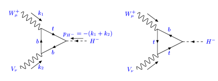
Figure 1: Top and bottom quark contributions to the one-loop $W^{+\mu}V^{\nu}H^{-}$ vertex, where $V=\gamma,Z$.

Explicit expressions for the form factors $G_{V}$, $H_{V}$ and $F_{V}$ are given in Appendix B.

The effective $W^{+}VH^{-}$ coupling gives both $t$-channel and $s$-channel contributions to the matrix element for $e^{+}e^{-}\to H^{+}e^{-}\bar{\nu}$, as shown in Fig. 2.

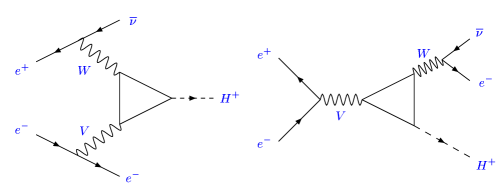
Figure 2: One-particle-irreducible contributions to $e^{+}e^{-}\to H^{+}e^{-}\bar{\nu}$ due to the fermion triangle diagram shown in Fig. 1.

The corresponding matrix elements can be written as

$$i\mathcal{M}_{\rm loop}^{t} = ie^{2}g_{W}\left[G_{V}g^{\mu\nu}+H_{V}k_{1}^{t\nu}k_{2}^{t\mu}+F_{V}i\epsilon^{\mu\nu\alpha\beta}k_{1\alpha}^{t}k_{2\beta}^{t}\right]$$ (2)

$$\times\frac{\bar{v}(e^{+}_{i})\gamma_{\mu}P_{L}v(\bar{\nu}_{f})\bar{u}(e^{-}_{f})\gamma_{\nu}(g^{eL}_{V}P_{L}+g^{eR}_{V}P_{R})u(e^{-}_{i})}{[k_{1}^{t2}-m_{W}^{2}][k_{2}^{t2}-m_{V}^{2}]}$$

$$i\mathcal{M}_{\rm loop}^{s} = ie^{2}g_{W}\left[G_{V}g^{\mu\nu}+H_{V}k_{1}^{s\nu}k_{2}^{s\mu}+F_{V}i\epsilon^{\mu\nu\alpha\beta}k_{1\alpha}^{s}k_{2\beta}^{s}\right]$$ (3)

$$\times\frac{\bar{u}(e^{-}_{f})\gamma_{\mu}P_{L}v(\bar{\nu}_{f})\bar{v}(e^{+}_{i})\gamma_{\nu}(g_{V}^{eL}P_{L}+g_{V}^{eR}P_{R})u(e^{-}_{i})}{[k_{1}^{s2}-m_{W}^{2}+im_{W}\Gamma_{W}][k_{2}^{s2}-m_{V}^{2}]},$$

where we use the notation $e^{-}_{i}\equiv p_{e^{-}_{i}}$, etc. The momenta $k_{1,2}^{t,s}$ are given by:

$$k_{1}^{t}=e^{+}_{i}-\bar{\nu}_{f},\qquad k_{2}^{t}=e^{-}_{i}-e^{-}_{f},$$

$$k_{1}^{s}=-e^{-}_{f}-\bar{\nu}_{f},\qquad k_{2}^{s}=e^{-}_{i}+e^{+}_{i}.$$ (4)

$P_{R,L}=(1\pm\gamma^{5})/2$ are the right- and left-handed projection operators. The gauge couplings $g_{W}$ and $g^{eL,R}_{V}$ are given in Appendix A. The additional contribution from the counterterm for the $W^{+}VH^{-}$ vertex is given in the next subsection.

II.2 Renormalization

We now compute the $H^{+}W^{+}$ and $H^{+}G^{+}$ mixing effects and renormalize the theory. A set of diagrams contributes to $e^{+}e^{-}\to H^{+}e^{-}\bar{\nu}$ in which a $W$ boson or charged Goldstone boson $G^{+}$ is radiated and turns into an $H^{+}$ through renormalized mixing diagrams. These are shown in Figs. 3 and 4 for the $t$- and $s$-channel processes, respectively, along with the $W^{+}H^{-}V$ coupling counterterm (denoted by an $X$) which renormalizes the $W^{+}H^{-}V$ vertex.

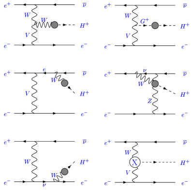
Figure 3: The $t$-channel mixing self-energy and counterterm contributions to $e^{+}e^{-}\to H^{+}e^{-}\bar{\nu}$. The shaded blob denotes the renormalized mixing self-energy and the $X$ denotes the $W^{+\mu}V^{\nu}H^{-}$ counterterm.

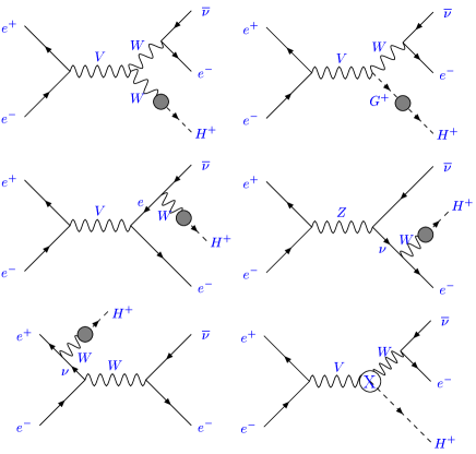
Figure 4: As in Fig. 3 but for the $s$-channel contributions.

We neglect all diagrams that are proportional to the electron or neutrino mass.

The top and bottom quark loops that give rise to the $W^{+}H^{+}$ and $G^{+}H^{+}$ mixing are shown in Fig. 5, along with their counterterms.

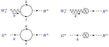
Figure 5: Top and bottom quark contributions to the $W^{+}H^{+}$ and $G^{+}H^{+}$ mixing (left) and the corresponding counterterms (right).

The $W^{+}H^{+}$ mixing diagram is denoted by $-ik^{\mu}\Sigma_{W^{+}H^{+}}(k^{2})$, where $k$ is the incoming momentum of the $W^{+}$ boson and $H^{+}$ is outgoing. The Hermitian conjugate diagram, with $H^{-}$ outgoing, has the opposite sign. The $G^{+}H^{+}$ mixing diagram is denoted by $+i\Sigma_{G^{+}H^{+}}(k^{2})$, where $k$ is the incoming momentum of the $G^{+}$ and $H^{+}$ is outgoing. The Hermitian conjugate diagram, with $H^{-}$ outgoing, is the same. The renormalized mixing two-point functions are denoted with a hat.

Because the process $e^{+}e^{-}\to H^{+}e^{-}\bar{\nu}$ is zero at tree level, the renormalization procedure is quite simple. In our discussion below, we follow the same on-shell renormalization scheme used in Ref. Arhrib . In fact, we need impose only the following two renormalization conditions. First, the renormalized tadpoles are set to zero. Second, the real part of the renormalized $W^{+}H^{+}$ mixing is set to zero when $H^{+}$ is on mass shell:

$${\rm Re}\,\hat{\Sigma}_{W^{+}H^{+}}(m^{2}_{H^{\pm}})=0.$$ (5)

This fixes the counterterm for $W^{+}H^{+}$ mixing shown in Fig. 5:

$$m_{W}\sin\beta\cos\beta\,\delta c={\rm Re}\,\Sigma_{W^{+}H^{+}}(m^{2}_{H^{\pm}}),$$ (6)

where $\delta c$ is a combination of counterterms (see, e.g., Ref. Dabelstein for the definitions of the counterterms):

$$\delta c\equiv\delta Z_{H_{1}}-\delta Z_{H_{2}}-\delta v_{1}/v_{1}+\delta v_{2}/v_{2}.$$ (7)

The renormalized $G^{+}H^{+}$ mixing two-point function, $\hat{\Sigma}_{G^{+}H^{+}}(k^{2})$, is fixed in terms of the renormalized $W^{+}H^{+}$ mixing two-point function $\hat{\Sigma}_{W^{+}H^{+}}(k^{2})$ by the Slavnov-Taylor identity (see, e.g., Refs. SlavnovTaylor ; SlavnovTaylor2 for details):

$$k^{2}\hat{\Sigma}_{W^{+}H^{+}}(k^{2})-m_{W}\hat{\Sigma}_{G^{+}H^{+}}(k^{2})=0.$$ (8)

Thus Eq. (5) also fixes the counterterm for $G^{+}H^{+}$ mixing shown in Fig. 5.

There is also a counterterm for the $W^{+\mu}V^{\nu}H^{-}$ vertex (all particles incoming), given by $-ig_{V}^{G}m_{W}\sin\beta\cos\beta\,\delta c\,g^{\mu\nu}$ and denoted by the $X$ in the last diagram of Figs. 3 and 4. The coupling $g_{V}^{G}$ is defined in Appendix A, Eq. (27). The counterterm for the Hermitian conjugate vertices, with $W^{-\mu}V^{\nu}H^{+}$ incoming, is identical. This counterterm $\delta c$ is also fixed by the condition in Eq. (5).

Applying these renormalization conditions, we find that the sum of the diagrams in Figs. 3 and 4 reduces to a quite simple result for both the $t$-channel and $s$-channel processes. See Appendix C for a detailed derivation. For the $t$-channel process, the sum of the diagrams in Fig. 3 is:

$$i\mathcal{M}_{\rm ren}^{t} = ie^{2}g_{W}\left[-g_{V}^{G}\Sigma_{W^{+}H^{+}}(m^{2}_{H^{\pm}})g^{\mu\nu}\right]$$

$$\hskip-28.45274pt\times\frac{\bar{v}(e^{+}_{i})\gamma_{\mu}P_{L}v(\bar{\nu}_{f})\bar{u}(e^{-}_{f})\gamma_{\nu}(g^{eL}_{V}P_{L}+g^{eR}_{V}P_{R})u(e^{-}_{i})}{[k_{1}^{t2}-m_{W}^{2}][k_{2}^{t2}-m_{V}^{2}]}.$$

For the $s$-channel process, the sum of the diagrams in Fig. 4 is:

$$i\mathcal{M}_{\rm ren}^{s} = ie^{2}g_{W}\left[-g_{V}^{G}\Sigma_{W^{+}H^{+}}(m^{2}_{H^{\pm}})g^{\mu\nu}\right]$$

$$\hskip-28.45274pt\times\frac{\bar{u}(e^{-}_{f})\gamma_{\mu}P_{L}v(\bar{\nu}_{f})\bar{v}(e^{+}_{i})\gamma_{\nu}(g_{V}^{eL}P_{L}+g_{V}^{eR}P_{R})u(e^{-}_{i})}{[k_{1}^{s2}-m_{W}^{2}+im_{W}\Gamma_{W}][k_{2}^{s2}-m_{V}^{2}]}.$$

Comparing these expressions to Eqs. (2) and (3), the sum of the counterterm and wavefunction renormalization diagrams can be written as a contribution to the form factor $G_{V}$, for both the $s$- and $t$-channel processes:

$$G_{V}^{\rm tot}=G_{V}^{\rm loop}-g_{V}^{G}\Sigma_{W^{+}H^{+}}(m^{2}_{H^{\pm}}).$$ (11)

The explicit expression for $\Sigma_{W^{+}H^{+}}(k^{2})$ is given in Appendix B.

One possible concern is that including the fixed $W$ decay width in the $W$ propagators for the $s$-channel diagrams might spoil the gauge invariance of the calculation. In our calculation, we use the “factorization scheme”, which is guaranteed to be gauge independent. Following, e.g., the discussion in Ref. nnHrcs , the one-loop matrix element in the factorization scheme is given by

$$\mathcal{M}=\frac{k_{1}^{s2}-m_{W}^{2}}{k_{1}^{s2}-m_{W}^{2}+im_{W}\Gamma_{W}}\mathcal{M}_{\Gamma_{W}=0},$$ (12)

which is exactly the relation that we used to obtain Eqs. (3) and (II.2).

II.3 Polarized cross sections

To compute the polarized cross sections, we first define the following combinations of form-factors:

$$(G,H,F)^{t,s}_{L,R}=\sum_{V=\gamma,Z}\frac{e^{2}g_{W}g_{V}^{eL,R}(G,H,F)_{V}}{[(k_{1}^{t,s})^{2}-m_{W}^{2}][(k_{2}^{t,s})^{2}-m_{V}^{2}]}.$$ (13)

The square of the matrix element is then given as follows. Because the $W$-boson couples only to left-handed fermions, the $t$-channel diagrams contribute only to $\mathcal{M}(e^{+}_{R}e^{-}_{L,R})$. Similarly, because of the vector coupling of $V=\gamma,Z$, the $s$-channel diagrams contribute only to $\mathcal{M}(e^{+}_{R}e^{-}_{L})$ and $\mathcal{M}(e^{+}_{L}e^{-}_{R})$. Thus, only the square of $\mathcal{M}(e^{+}_{R}e^{-}_{L})$ will involve interference between the $s$- and $t$-channel diagrams, and $\mathcal{M}(e^{+}_{L}e^{-}_{L})$ is zero. In particular, we have:

$$|{\cal{M}}(e^{+}_{R}e^{-}_{L})|^{2}=K_{L}^{t}+K_{L}^{s}+K^{st},\quad|{\cal{M}}(e^{+}_{L}e^{-}_{R})|^{2}=K_{R}^{s},$$

$$|{\cal{M}}(e^{+}_{R}e^{-}_{R})|^{2}=K_{R}^{t},\quad|{\cal{M}}(e^{+}_{L}e^{-}_{L})|^{2}=0,$$ (14)

where $K_{L,R}^{t}$, $K_{L,R}^{s}$ and $K^{st}$ are given in Appendix B in terms of the form-factors in Eq. (13).

III Numerical results

In this section, we present our numerical results for the cross section of $e^{+}e^{-}\rightarrow H^{+}e^{-}\bar{\nu}$. We have used the LoopTools package LoopTools to compute the one-loop integrals. The electron and positron beams are assumed to be unpolarized unless specified explicitly. Also, we plot the cross section for $e^{+}e^{-}\to H^{+}e^{-}\bar{\nu}$ only. The cross section for the charge-conjugate process is the same (for unpolarized beams); adding them together doubles the cross sections shown.

We first show the $\tan\beta$ dependence of the cross section for fixed $m_{H^{\pm}}=\sqrt{s}/2$ in Figs. 6 ($\sqrt{s}=500$ GeV) and 7 ($\sqrt{s}=1000$ GeV).

Figure 6: Cross section for $e^{+}e^{-}\to H^{+}e^{-}\bar{\nu}$ as a function of $\tan\beta$ for $\sqrt{s}=500$ GeV and $m_{H^{\pm}}=250$ GeV. We show the total cross section (solid line), $s$-channel contribution (dashed line) and $t$-channel contribution (dotted line).

Figure 7: As in Fig. 6 but for $\sqrt{s}=1000$ GeV and $m_{H^{\pm}}=500$ GeV.

The cross section falls like $(\tan\beta)^{-2}$ due to the factor of $y^{L}_{Htb}\propto\cot\beta$ in the matrix elements. At very large $\tan\beta$ values the cross section begins to turn upward again due to terms proportional to $y^{R}_{Htb}\propto\tan\beta$ in the matrix elements. This effect is barely visible at $\tan\beta=40$ in Fig. 6. At a 500 GeV LC, the cross section for a charged Higgs boson with 250 GeV mass is larger than 0.01 fb (corresponding to 10 events for integrated luminosity ${\cal L}=500\ {\rm fb}^{-1}$ when both $H^{+}$ and $H^{-}$ are taken into account) only for small $\tan\beta<1.7$.

From Figs. 6 and 7 we can also see that at $\sqrt{s}=500$ GeV, the $s$-channel contribution dominates the total cross section, while at $\sqrt{s}=1000$ GeV, the $s$- and $t$- channel contributions become comparable. This center-of-mass energy dependence of the cross section can be seen in Fig. 8, which shows the $s$-channel (dashed line) and $t$-channel (dotted line) contributions versus center-of-mass energy for $m_{H^{\pm}}=\sqrt{s}/2$ and $\tan\beta=2.5$.

Figure 8: Cross section as a function of $\sqrt{s}$ for $m_{H^{\pm}}=\sqrt{s}/2$ and $\tan\beta=2.5$, to show different behavior of $s$-channel and $t$-channel contributions.

The $t$-channel contribution dominates when $\sqrt{s}>1050$ GeV. This crossover happens at a higher center-of-mass energy than in the case of the similar process $e^{+}e^{-}\rightarrow\nu\bar{\nu}A^{0}$, for which the $t$-channel dominates when $\sqrt{s}>670$ GeV nunuA . In general, the $t$-channel contribution becomes more important than the $s$-channel contribution at larger $\sqrt{s}$ values because of the propagator suppression $\sim 1/s$ of the $s$-channel contribution. In the process $e^{+}e^{-}\rightarrow\nu\bar{\nu}A^{0}$, there is an additional enhancement of the $t$-channel contribution from the fact that the $W^{+}e^{-}\bar{\nu}$ coupling in the $t$-channel process is larger than the $Ze^{+}e^{-}$ and $Z\nu\bar{\nu}$ couplings in the $s$-channel process. This makes the $t$-channel contribution start to dominate at a smaller $\sqrt{s}$ value in $e^{+}e^{-}\rightarrow\nu\bar{\nu}A^{0}$ than in $e^{+}e^{-}\rightarrow H^{+}e^{-}\bar{\nu}$, where such additional enhancement from the relevant couplings does not occur.

We also show the charged Higgs mass dependence of the cross section for an unpolarized electron beam (Fig. 9) and an 80% left-polarized electron beam (Fig. 10).

Figure 9: Cross section as a function of $m_{H^{\pm}}$ for $\tan\beta=2.5$ and $\sqrt{s}=500$ GeV.

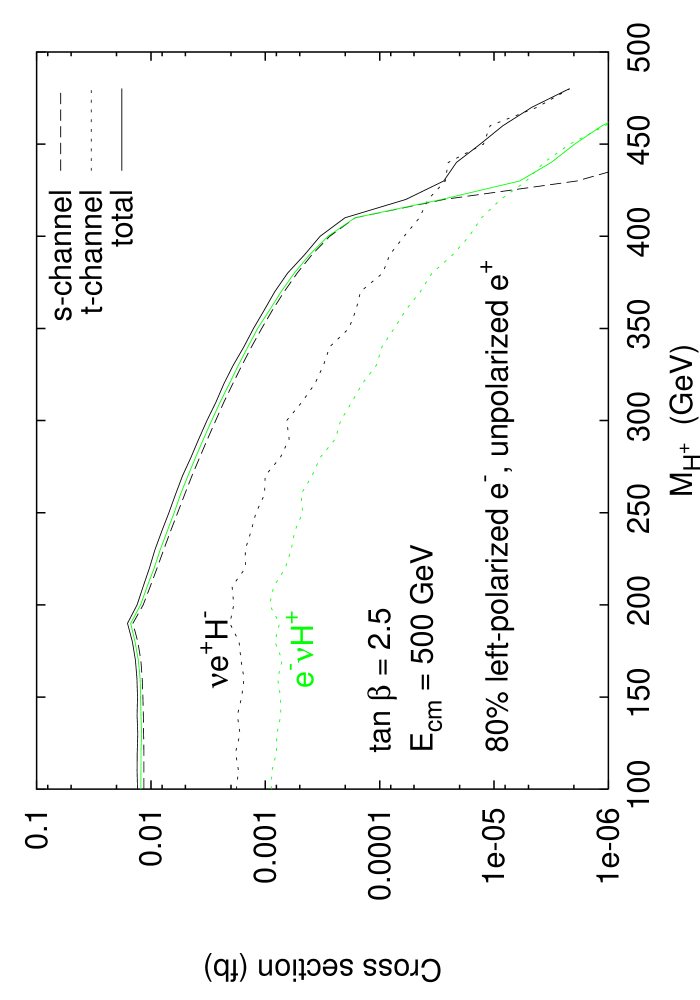
Figure 10: As in Fig. 9 but with an 80% left-polarized $e^{-}$ beam. The $t$-channel contribution is now different for the $H^{+}e^{-}\bar{\nu}$ and $H^{-}e^{+}\nu$ final states, as indicated by the green (gray) and black lines, respectively. Notice that there are two solid lines for total cross section, corresponding to $H^{+}e^{-}\bar{\nu}$ and $H^{-}e^{+}\nu$ respectively.

With a polarized electron beam (and unpolarized positron beam), the $t$-channel contribution to the $e^{+}e^{-}\to H^{+}e^{-}\bar{\nu}$ cross section is different from that to the $e^{+}e^{-}\to H^{-}e^{+}\nu$ cross section. This is because for $e^{+}e^{-}\to H^{+}e^{-}\bar{\nu}$, the $t$-channel $W$ boson couples to the positron beam, while for $e^{+}e^{-}\to H^{-}e^{+}\nu$ it couples to the electron beam. Left-polarizing the electron beam thus has a much more sizable effect on the $t$-channel $e^{+}e^{-}\to H^{-}e^{+}\nu$ cross section, enhancing it significantly. Left-polarizing the electron beam causes a slight suppression of the $t$-channel $e^{+}e^{-}\to H^{+}e^{-}\bar{\nu}$ cross section, due to the relative size of the sum of the photon and $Z$ exchange diagrams for left- and right-handed electrons. The $s$-channel contribution is identical for the two final states; it is enhanced by about 50% with an 80% left-polarized $e^{-}$ beam, which is consistent with the results for the process $e^{+}e^{-}\rightarrow H^{+}W^{-}$ HW .

We summarize the results of Figs. 6 and 9 in Fig. 11, where we show contours of cross section for $e^{+}e^{-}\to H^{+}e^{-}\bar{\nu}$ in the $m_{H^{\pm}}-\tan\beta$ plane.

Figure 11: Cross section in the $m_{H^{\pm}}-\tan\beta$ plane for unpolarized beams with $\sqrt{s}=500$ GeV. The vertical dotted line indicates the pair production threshold, $m_{H^{\pm}}=\sqrt{s}/2=250$ GeV.

A cross section above 0.1 fb corresponds to 100 charged Higgs events (combining $H^{+}$ and $H^{-}$) in an integrated luminosity of 500 fb^-1. This occurs mainly only for $m_{H^{\pm}}<\sqrt{s}/2$, and thus would not aid in the charged Higgs discovery. It could, however, be useful for measuring $\tan\beta$ at low $\tan\beta$ values, due to the strong $(\tan\beta)^{-2}$ dependence of the cross section. The $e^{+}e^{-}\to H^{+}e^{-}\bar{\nu}$ events could be separated from $e^{+}e^{-}\to H^{+}H^{-}$ events by using the fact that $H^{-}\to e^{-}\bar{\nu}$ is suppressed by the tiny electron Yukawa coupling. A cross section above 0.01 fb corresponds to 10 charged Higgs events (again combining $H^{+}$ and $H^{-}$) in 500 fb^-1, and is probably the limit of relevance of this process. It offers some reach for $m_{H^{\pm}}>\sqrt{s}/2$ for low $\tan\beta$ values below 1.7. The statistics could be roughly doubled by including the $H^{+}\mu^{-}\bar{\nu}$ and $H^{-}\nu\mu^{+}$ final states, which receive only $s$-channel contributions and have the same $s$-channel cross section as the process with an electron or positron in the final state.

Since the $s$-channel contribution dominates the total cross section for $\sqrt{s}\mathrel{\raise 1.29167pt\hbox{$<$\kern-7.5pt\lower 4.30554pt\hbox{$\sim$}}}1000$ GeV, we show the comparison of the cross section for $e^{+}e^{-}\to H^{+}e^{-}\bar{\nu}$ with that of the resonant process $e^{+}e^{-}\to H^{+}W^{-}$ (with $W^{-}\to e^{-}\bar{\nu}$) in Fig. 12.

Figure 12: Comparison of the cross section for $e^{+}e^{-}\to H^{+}e^{-}\bar{\nu}$ with the resonant process $e^{+}e^{-}\to H^{+}W^{-}$, with $W^{-}\to e^{-}\bar{\nu}$. Here we plot the cross section on a linear scale so that the difference between the full $s$-channel contribution and the resonant sub-diagrams will be visible.

In the $e^{+}e^{-}\to H^{+}W^{-}$ cross section calculation we include only the top and bottom quark loops and we use the tree-level result for the branching ratio of $W^{-}\to e^{-}\bar{\nu}$ in order to make a consistent comparison. The resonant contribution is about 80% of the full $s$-channel cross section.

IV Model dependence

Here we discuss the model dependence of our results, and show how they can be extended beyond our current calculations.

IV.1 Higgs potential

Since we have included only the top and bottom quark loops in our calculation, our results are valid regardless of the form of the Higgs potential for the 2HDM. Once the contributions of gauge and Higgs boson loops are included, however, the cross section will depend on the form of the Higgs potential through the Higgs boson self-couplings. As shown in Ref. Kanemura , the effect of the gauge and Higgs boson loops on the $e^{+}e^{-}\to H^{+}W^{-}$ cross section is negligible unless the Higgs boson self couplings are very large; even then, the gauge and Higgs boson loops only become important for $\tan\beta\mathrel{\raise 1.29167pt\hbox{$>$\kern-7.5pt\lower 4.30554pt\hbox{$\sim$}}}4$, where the cross section has already fallen off by more than an order of magnitude compared to $\tan\beta=1$. Thus, even if the Higgs boson self-couplings are large, we do not expect the gauge and Higgs boson loops to be important when the cross section is large enough to be observed.

IV.2 Type I vs. Type II 2HDM

In our numerical results we have assumed that the Higgs sector is the Type II 2HDM, in which one Higgs doublet gives mass to the up-type quarks and the other Higgs doublet gives mass to the down-type quarks and the charged leptons. In the Type I 2HDM, one Higgs doublet gives mass to all fermions. In this case, all our results remain the same except that $y^{R}_{Htb}$ in Eq. (28) is modified to

$$y^{R}_{Htb}=\frac{m_{b}\cot\beta}{\sqrt{2}m_{W}s_{W}}\qquad{\rm(Type\ I)}.$$ (15)

The effect of this is that the curves in Fig. 6 do not start to flatten out at high $\tan\beta$. The results at low $\tan\beta$ are unchanged. Thus, to a very good approximation, our results are valid also for the Type I 2HDM, except at large $\tan\beta$.

IV.3 Higgs sector extensions beyond the 2HDM

We may also consider the effects of extending the Higgs sector beyond the 2HDM. Adding neutral Higgs singlets can only affect the gauge and Higgs boson loops, which we have argued are unlikely to be experimentally relevant. Adding charged Higgs bosons via additional doublets or charged singlets leads to a Higgs sector with more than one charged Higgs boson, the lightest of which will in general be a mixture of the various gauge eigenstates. To avoid Higgs-mediated flavor changing neutral currents, fermions of each charge should couple to no more than one Higgs doublet noTypeIII . Thus the mixing will in general lead to a suppression of the lightest $H^{\pm}$ couplings to top and bottom quarks; the effect will be the same as increasing $\tan\beta$ in the Type I model.

Adding larger Higgs multiplets leads to more interesting effects. For example, adding a Higgs triplet with a nonzero vacuum expectation value leads to a nonzero $W^{+}ZH^{-}$ coupling at tree level. This tree-level $W^{+}ZH^{-}$ coupling is proportional to the triplet vacuum expectation value $v_{3}$:

$$g_{W^{+}ZH^{-}}=\left\{\begin{array}[]{lcl}g^{2}(c^{2}_{W}-2)v_{3}/\sqrt{2}c_{W}&&{\rm complex\ triplet}\\ g^{2}c_{W}v_{3}&&{\rm real\ triplet}.\end{array}\right.$$ (16)

The triplet vacuum expectation value is forced to be small by the experimental constraints on weak isospin violation:

$$\delta\rho=\left\{\begin{array}[]{lcl}-2v_{3}^{2}/v_{SM}^{2}&&{\rm complex\ triplet}\\ 4v_{3}^{2}/v_{SM}^{2}&&{\rm real\ triplet}.\end{array}\right.$$ (17)

The current constraint on contributions to the $\rho$ parameter from new physics is $-0.0016<\Delta\rho<0.0058$ at the $2\sigma$ level PDG . This leads to an upper bound on the tree-level cross section for $e^{+}e^{-}\to H^{+}e^{-}\bar{\nu}$ of 0.0035 fb for a real triplet, or 0.0026 fb for a complex triplet, with $m_{H^{+}}=250$ GeV at $\sqrt{s}=500$ GeV and assuming unpolarized beams. This corresponds to 3.5 events (counting $H^{+}$ and $H^{-}$ final states) in 500 fb^-1 of integrated luminosity for a real triplet, and 2.6 events for a complex triplet, both of which are too small to be observable. From Fig. 6, these cross sections become comparable to the loop-induced cross section in the 2HDM at $\tan\beta\simeq 3-3.5$.

IV.4 MSSM

In the MSSM, this process will get contributions from SUSY loops, just as $e^{+}e^{-}\to H^{+}W^{-}$ does. In the latter case, the SUSY loops could increase the cross section by 50-100% at low $\tan\beta$ if the SUSY particles are relatively light HWupdate . Since the resonant $e^{+}e^{-}\to H^{+}W^{-}$ subprocess dominates the cross section at $\sqrt{s}\mathrel{\raise 1.29167pt\hbox{$<$\kern-7.5pt\lower 4.30554pt\hbox{$\sim$}}}1000$ GeV, we expect this enhancement to carry over. In the MSSM, however, $\tan\beta$ is limited to be above 2.4 LEP2 , which already leads to a somewhat smaller cross section.

A different source of SUSY corrections to the $e^{+}e^{-}\to H^{+}e^{-}\bar{\nu}$ cross section is the SUSY radiative correction to the bottom quark Yukawa coupling, parameterized by $\Delta_{b}$ Deltab . This correction arises from a coupling of the second Higgs doublet $\Phi_{2}$ to the bottom quark induced at one-loop by SUSY-breaking terms:

$$-\mathcal{L}_{\rm Yukawa}\simeq h_{b}\Phi_{1}^{0}\bar{b}b+(\Delta h_{b})\Phi_{2}^{0}\bar{b}b.$$ (18)

While $\Delta h_{b}$ is one-loop suppressed compared to $h_{b}$, for sufficiently large $\tan\beta\equiv v_{2}/v_{1}$ the contribution of both terms in Eq. (18) to the $b$ quark mass can be comparable in size. This leads to a large modification of the tree-level relation for the bottom quark mass,

$$m_{b}=\frac{h_{b}v_{1}}{\sqrt{2}}(1+\Delta_{b}),$$ (19)

where $\Delta_{b}\equiv(\Delta h_{b})\tan\beta/h_{b}$. The correction $\Delta_{b}$ comes from two main sources: (1) a bottom squark–gluino loop, which depends on the masses $m_{\tilde{b}_{1,2}}$ of the two bottom squarks and the gluino mass $m_{\tilde{g}}$; and (2) a top squark–Higgsino loop, which depends on the masses $m_{\tilde{t}_{1,2}}$ of the two top squarks and the Higgsino mass parameter $\mu$. Neglecting contributions proportional to the electroweak gauge couplings, we have explicitly Deltab :

$$\Delta_{b} \simeq \frac{2\alpha_{s}}{3\pi}m_{\tilde{g}}\mu\tan\beta\ I(m_{\tilde{b}_{1}},m_{\tilde{b}_{2}},m_{\tilde{g}})$$ (20)

$$+\frac{Y_{t}}{4\pi}A_{t}\mu\tan\beta\ I(m_{\tilde{t}_{1}},m_{\tilde{t}_{2}},\mu).$$

Here $A_{t}$ is the trilinear coupling in the top squark sector, $\alpha_{s}=g_{s}^{2}/4\pi$, and $Y_{t}\equiv h_{t}^{2}/4\pi$. The loop function $I$ is positive definite. Since the Higgs coupling $\Delta h_{b}$ is a manifestation of SUSY breaking, it does not decouple in the limit of large SUSY breaking mass parameters. In fact, if all SUSY breaking mass parameters and $\mu$ are scaled by a common factor, $\Delta_{b}$ remains constant. These corrections modify $y^{R}_{Htb}$ in Eq. (28):

$$y^{R}_{Htb}=\frac{m_{b}\cot\beta}{\sqrt{2}m_{W}s_{W}}\frac{1}{1+\Delta_{b}}\qquad({\rm MSSM}).$$ (21)

To explore the impact of these effects, we plot the cross section for $e^{+}e^{-}\to H^{+}e^{-}\bar{\nu}$ in Fig. 13 with the specific choices of $m_{H^{+}}=250$ GeV, $\sqrt{s}=500$ GeV, $\mu=-2$ TeV, $m_{\tilde{b}_{R}}=525$ GeV, $m_{\tilde{g}}=m_{\tilde{b}_{L}}=m_{\tilde{t}_{L,R}}=1$ TeV, and $A_{t}=A_{b}=\mu/\tan\beta+\sqrt{6}m_{\tilde{t}_{L}}$ (corresponding to maximal-mixing in the top squark sector), and compare to the result that would be obtained without including $\Delta_{b}$. For these input parameters, $\Delta_{b}$ varies between $-\tan\beta/26$ and $-\tan\beta/22$ for $\tan\beta$ between 1 and 50.

Figure 13: Cross section for $e^{+}e^{-}\to H^{+}e^{-}\bar{\nu}$ as a function of $\tan\beta$ for $\sqrt{s}=500$ GeV and $m_{H^{\pm}}=250$ GeV. The MSSM parameters are specified in the text. In the region near $\Delta_{b}=-1$, we cut off the divergence by requiring $e|y^{R}_{Htb}|\leq 4\pi$. The dotted line shows the total cross section for $\Delta_{b}=0$.

For $\Delta_{b}\simeq-1$ the resulting $y^{R}_{Htb}$ becomes quite large, making our perturbative results unreliable. To control such effects we cut off the divergence in this region by requiring $e|y^{R}_{Htb}|\leq 4\pi$. The dip in the cross section at $\tan\beta\simeq 20$ is due to destructive interference between various terms, which changes to constructive interference for $\tan\beta>22$ where $\Delta_{b}<-1$ and $y^{R}_{Htb}$ has the opposite sign than in the SM case. While the modification of the cross section due to $\Delta_{b}$ can be quite significant, it occurs at large $\tan\beta$ where the cross section is already very small, and thus is unlikely to be observable for perturbative values of $y^{R}_{Htb}$.

V Conclusions

We have computed the cross section for $e^{+}e^{-}\to H^{+}e^{-}\bar{\nu}$, from one-loop diagrams involving top and bottom quarks in the Type II two-Higgs-doublet model. This process is interesting because it offers an opportunity to produce the charged Higgs boson in $e^{+}e^{-}$ collisions for charged Higgs masses above half of the collider center-of-mass energy. Because this process first appears at the one-loop level, however, its cross section is very small. At low values of $\tan\beta\sim 1-2$ the cross section can reach the 0.01 fb level at $\sqrt{s}=500$ GeV and $m_{H^{\pm}}=250$ GeV, leading to 10 events in 500 fb^-1 when the cross sections for $H^{+}$ and $H^{-}$ production are combined. Using an 80% left-polarized $e^{-}$ beam increases the cross section by about 50%. The cross section falls with increasing $\tan\beta$ like $(\tan\beta)^{-2}$.

The process $e^{+}e^{-}\to H^{+}e^{-}\bar{\nu}$ receives contributions from $s$-channel and $t$-channel diagrams, which behave differently with increasing center-of-mass energy. The $s$-channel contribution dominates at low $\sqrt{s}\mathrel{\raise 1.29167pt\hbox{$<$\kern-7.5pt\lower 4.30554pt\hbox{$\sim$}}}1$ TeV, while the $t$-channel contribution dominates at higher energies. The $s$-channel contribution is in turn dominated (at the 80% level) by the resonant sub-process, $e^{+}e^{-}\to H^{+}W^{-}$, with $W^{-}\to e^{-}\bar{\nu}$. Because of this, in the context of the MSSM we expect the effects of light superpartners calculated for the $e^{+}e^{-}\to H^{+}W^{-}$ cross section to carry over to the process $e^{+}e^{-}\to H^{+}e^{-}\bar{\nu}$. Light superpartners can lead to an increase in the $e^{+}e^{-}\to H^{+}W^{-}$ cross section by 50-100% at low $\tan\beta$.

The final state containing $e^{-}\bar{\nu}$ is experimentally attractive because it is easy to tag compared to hadronic $W$ decays. To increase the statistics, one could also include the $e^{+}e^{-}\to H^{+}\mu^{-}\bar{\nu}$ channel, which comes only from the $s$-channel diagrams. This would roughly double the cross section at $\sqrt{s}=500$ GeV, where the $t$-channel process does not contribute significantly. The processes $e^{+}e^{-}\to H^{+}q\bar{q}^{\prime}$ for the first two generations of quarks could also be included (analogous to including hadronic $W$ decays); it would then contribute another six times the $s$-channel cross section of the electron mode. For the third generation, $e^{+}e^{-}\to H^{+}\tau^{-}\bar{\nu}$ and $e^{+}e^{-}\to H^{+}\bar{t}b$, however, the tree level contributions dominate due to the relatively large Yukawa couplings. Such channels have already been studied in tbHtaunuH .

For $m_{H^{\pm}}<\sqrt{s}/2$, where the charged Higgs boson can be pair produced, the process $e^{+}e^{-}\to H^{+}e^{-}\bar{\nu}$ could still be useful to measure $\tan\beta$ due to the strong $(\tan\beta)^{-2}$ dependence of the cross section. This process should be separable from the pair production process since the $H^{-}$ decay to $e^{-}\bar{\nu}$ is suppressed by the tiny electron Yukawa coupling.

Appendix A Notation and conventions

For the one-loop integrals we follow the notation of Ref. LoopTools . The one-point integral is:

$$\frac{i}{16\pi^{2}}A(m^{2})=\int\!\frac{d^{D}q}{(2\pi)^{D}}\frac{1}{(q^{2}-m^{2})},$$ (22)

where $D$ is the number of dimensions. The two-point integrals are:

$$\frac{i}{16\pi^{2}}\left\{B_{0},k^{\mu}B_{1}\right\}(k^{2},m_{0}^{2},m_{1}^{2})=$$ (23)

$$\hskip 28.45274pt\int\!\frac{d^{D}q}{(2\pi)^{D}}\frac{\{1,q^{\mu}\}}{(q^{2}-m_{0}^{2})((q+k)^{2}-m_{1}^{2})}.$$

The three-point integrals are:

$$\frac{i}{16\pi^{2}}\left\{C_{0},C^{\mu},C^{\mu\nu}\right\}=$$ (24)

$$\hskip 0.0pt\int\!\frac{d^{D}q}{(2\pi)^{D}}\frac{\{1,q^{\mu},q^{\mu}q^{\nu}\}}{(q^{2}-m_{0}^{2})((q+k_{1})^{2}-m_{1}^{2})((q+k_{2})^{2}-m_{2}^{2})},$$

where the tensor integrals are decomposed in terms of scalar components as

$$C^{\mu} = k_{1}^{\mu}C_{1}+k_{2}^{\mu}C_{2}$$

$$C^{\mu\nu} = g^{\mu\nu}C_{00}+k_{1}^{\mu}k_{1}^{\nu}C_{11}+k_{2}^{\mu}k_{2}^{\nu}C_{22}$$ (25)

$$+(k_{1}^{\mu}k_{2}^{\nu}+k_{2}^{\mu}k_{1}^{\nu})C_{12}.$$

The arguments of the scalar three-point integrals are $(k_{1}^{2},(k_{2}-k_{1})^{2},k_{2}^{2},m_{0}^{2},m_{1}^{2},m_{2}^{2})$.

For couplings and Feynman rules we follow the conventions of Ref. HaberKane . The photon and $Z$ boson coupling coefficients to fermions are:

$$g_{\gamma}^{fL}=g_{\gamma}^{fR}=-e_{f},$$ (26)

$$g_{Z}^{fL}=(-T_{3}+e_{f}s_{W}^{2})/s_{W}c_{W},\quad g_{Z}^{fR}=(e_{f}s_{W}^{2})/s_{W}c_{W},$$

where the electric charges are $e_{\nu}=0$, $e_{e}=-1$, $e_{u}=2/3$, and $e_{d}=-1/3$ and where $T_{3}=1/2$ for $\nu$, $u$ and $T_{3}=-1/2$ for $e$, $d$.

For the $W$ and $Z$ boson and photon couplings to fermions and the Goldstone boson we define:

$$g_{W}=-1/\sqrt{2}s_{W},\quad g_{\gamma}=-e,\quad g_{Z}=-ec_{W}/s_{W},$$

$$g^{G}_{\gamma}=e,\quad g^{G}_{Z}=-es_{W}/c_{W}.$$ (27)

Finally, the $H^{\pm}$ coupling coefficients to top and bottom quarks are:

$$y^{L}_{Htb}=\frac{m_{t}\cot\beta}{\sqrt{2}m_{W}s_{W}},\qquad y^{R}_{Htb}=\frac{m_{b}\tan\beta}{\sqrt{2}m_{W}s_{W}}.$$ (28)

Appendix B Matrix elements

B.1 Top and bottom quark contributions

The $W^{+}H^{+}$ mixing diagram (Fig. 5) was given in Refs. Arhrib ; Kanemura ; HW :

$$\Sigma_{W^{+}H^{+}}(k^{2}) = \frac{N_{c}\alpha}{2\pi}g_{W}\left[(m_{t}y^{L}_{Htb}+m_{b}y^{R}_{Htb})B_{1}\right.$$ (29)

$$\qquad\left.+m_{b}y^{R}_{Htb}B_{0}\right],$$

with the arguments of the two-point integrals given by $B(k^{2},m_{b}^{2},m_{t}^{2})$.

The top and bottom quark contributions to the effective $W^{+}_{\mu}V_{\nu}H^{-}$ coupling are shown in Fig. 1. The corresponding form-factors $G_{V}$, $H_{V}$ and $F_{V}$ can be read off from the $s$-channel matrix element for $e^{+}e^{-}\to W^{+}H^{-}$ given in Refs. Arhrib ; Kanemura ; HW using the following relation:

$$i\mathcal{M} = \frac{ie}{s-m_{V}^{2}}\left\{G_{V}[g_{V}^{eR}\mathcal{A}_{1}+g_{V}^{eL}\mathcal{A}_{2}]-H_{V}[g_{V}^{eR}(\mathcal{A}_{3}+\mathcal{A}_{5})+g_{V}^{eL}(\mathcal{A}_{4}+\mathcal{A}_{6})]+F_{V}[g_{V}^{eR}\mathcal{A}_{7}+g_{V}^{eL}\mathcal{A}_{8}]\right\},$$ (30)

where the $\mathcal{A}_{i}$ are matrix elements defined in Refs. Arhrib ; HW . The loop involving $t,b,b$ gives:

$$G_{V} = \frac{e\alpha N_{c}g_{W}}{2\pi}\left[-(m_{t}g_{V}^{dL}y_{Htb}^{L}+m_{b}(g_{V}^{dL}-g_{V}^{dR})y_{Htb}^{R})B_{0}+2g_{V}^{dL}(m_{t}y_{Htb}^{L}+m_{b}y_{Htb}^{R})C_{00}\right.$$

$$\left.+(-g_{V}^{dL}(m_{t}y_{Htb}^{L}+m_{b}y_{Htb}^{R})k_{1}^{2}+(m_{t}g_{V}^{dL}y_{Htb}^{L}-m_{b}g_{V}^{dR}y_{Htb}^{R})(-k_{1}^{2}-k_{1}\cdot k_{2}))C_{1}\right.$$

$$\left.+(g_{V}^{dL}(m_{t}y_{Htb}^{L}+m_{b}y_{Htb}^{R})(-k_{1}^{2}-k_{1}\cdot k_{2})-(m_{t}g_{V}^{dL}y_{Htb}^{L}-m_{b}g_{V}^{dR}y_{Htb}^{R})m_{H^{\pm}}^{2})C_{2}\right.$$

$$\left.+(-m_{t}^{3}g_{V}^{dL}y_{Htb}^{L}-m_{t}^{2}m_{b}(g_{V}^{dL}-g_{V}^{dR})y_{Htb}^{R}+m_{t}m_{b}^{2}g_{V}^{dR}y_{Htb}^{L}+m_{t}g_{V}^{dL}y_{Htb}^{L}(-k_{1}^{2}-k_{1}\cdot k_{2}))C_{0}\right]$$

$$H_{V} = -\frac{e\alpha N_{c}g_{W}}{2\pi}\left[-2g_{V}^{dL}(m_{t}y_{Htb}^{L}+m_{b}y_{Htb}^{R})(C_{12}+C_{22})-g_{V}^{dL}(3m_{t}y_{Htb}^{L}+m_{b}y_{Htb}^{R})C_{2}-(m_{t}g_{V}^{dL}y_{Htb}^{L}-m_{b}g_{V}^{dR}y_{Htb}^{R})C_{1}\right.$$

$$\left.-m_{t}g_{V}^{dL}y_{Htb}^{L}{C}_{0}\right]$$

$$F_{V} = \frac{e\alpha N_{c}g_{W}}{2\pi}\left[m_{t}g_{V}^{dL}y_{Htb}^{L}{C}_{0}+(m_{t}g_{V}^{dL}y_{Htb}^{L}+m_{b}g_{V}^{dR}y_{Htb}^{R})C_{1}+g_{V}^{dL}(m_{t}y_{Htb}^{L}+m_{b}y_{Htb}^{R})C_{2}\right]$$ (31)

with the arguments for the integral functions as $B(k_{2}^{2},m_{b}^{2},m_{b}^{2})$, $C(k_{1}^{2},k_{2}^{2},m_{H^{\pm}}^{2},m_{t}^{2},m_{b}^{2},m_{b}^{2})$. The contributions of the loop involving $t,t,b$ are given by the substitutions:

$$m_{t}\leftrightarrow m_{b},\ \ g_{V}^{dL}\leftrightarrow g_{V}^{uL},\ \ \ g_{V}^{dR}\leftrightarrow g_{V}^{uR},\ \ \ y_{Htb}^{L}\leftrightarrow y_{Htb}^{R};$$

and $F_{V}$ gets an overall minus sign.

B.2 Square of the matrix element

The square of the matrix element is given as follows in terms of the form-factors $(G,H,F)_{L,R}^{t,s}$ defined in Eq. (13).

We define the following kinematic variables:

$$s=2e^{-}_{i}\cdot e^{+},\quad\hat{s}=2e^{-}_{f}\cdot\bar{\nu},\quad t_{1}=-2e^{-}_{i}\cdot e^{-}_{f},$$

$$t_{2}=-2e^{+}\cdot\bar{\nu},\quad u_{1}=-2e^{-}_{i}\cdot\bar{\nu},\quad u_{2}=-2e^{+}\cdot e^{-}_{f}\,,$$

$$\epsilon(e^{-}_{i},e^{+},e^{-}_{f},\bar{\nu})=\epsilon^{\mu\nu\rho\sigma}(e^{-}_{i})_{\mu}\,e^{+}_{\nu}\,(e^{-}_{f})_{\rho}\bar{\nu}_{\sigma}\,.$$ (32)

For the antisymmetric tensor we use the convention $\epsilon^{0123}=+1$.

The squares of the matrix elements $K^{t}_{L,R}$, $K^{s}_{L,R}$, and $K^{st}$ are given as follows.

$K_{L}^{t}$ is given by:

$$K_{L}^{t} = 4|G_{L}^{t}|^{2}u_{1}u_{2}$$ (33)

$$+ |H_{L}^{t}|^{2}(s\hat{s}-t_{1}t_{2}+u_{1}u_{2}+su_{1}+\hat{s}u_{2})(s\hat{s}-t_{1}t_{2}+u_{1}u_{2}+su_{2}+\hat{s}u_{1})$$

$$+ |F_{L}^{t}|^{2}(-s^{2}\hat{s}^{2}-t_{1}^{2}t_{2}^{2}-u_{1}^{2}u_{2}^{2}+2s\hat{s}t_{1}t_{2}+2s\hat{s}u_{1}u_{2}+t_{1}t_{2}u_{1}^{2}+t_{1}t_{2}u_{2}^{2})$$

$$+ 2{\rm Re}(G_{L}^{t}H_{L}^{t*})(u_{1}^{2}u_{2}+u_{1}u_{2}^{2}+s\hat{s}u_{1}+s\hat{s}u_{2}+2su_{1}u_{2}+2\hat{s}u_{1}u_{2}-t_{1}t_{2}u_{1}-t_{1}t_{2}u_{2})$$

$$+ 8{\rm Im}(G_{L}^{t}H_{L}^{t*})\epsilon(e^{-}_{i},e^{+},e^{-}_{f},\bar{\nu})(u_{1}-u_{2})$$

$$+ 2{\rm Re}(G_{L}^{t}F_{L}^{t*})(u_{1}^{2}u_{2}-u_{1}u_{2}^{2}-s\hat{s}u_{1}+s\hat{s}u_{2}+t_{1}t_{2}u_{1}-t_{1}t_{2}u_{2})$$

$$- 8{\rm Im}(G_{L}^{t}F_{L}^{t*})\epsilon(e^{-}_{i},e^{+},e^{-}_{f},\bar{\nu})(u_{1}+u_{2})$$

$$- {\rm Re}(H_{L}^{t}F_{L}^{t*})(u_{1}-u_{2})(s^{2}\hat{s}+s\hat{s}^{2}-u_{1}^{2}u_{2}-u_{1}u_{2}^{2}+s\hat{s}u_{1}+s\hat{s}u_{2}$$

$$-st_{1}t_{2}-\hat{s}t_{1}t_{2}-su_{1}u_{2}-\hat{s}u_{1}u_{2}+t_{1}t_{2}u_{1}+t_{1}t_{2}u_{2})$$

$$- 4{\rm Im}(H_{L}^{t}F_{L}^{t*})\epsilon(e^{-}_{i},e^{+},e^{-}_{f},\bar{\nu})(2s\hat{s}-2t_{1}t_{2}+u_{1}^{2}+u_{2}^{2}+su_{1}+\hat{s}u_{1}+su_{2}+\hat{s}u_{2}).$$

$K_{R}^{t}$ can be obtained from Eq. (33) by the substitutions $u_{1}\leftrightarrow s$ and $u_{2}\leftrightarrow\hat{s}$, with an additional minus sign for the $G^{t}F^{t*}$ and $H^{t}F^{t*}$ terms:

$$K_{R}^{t} = 4|G_{R}^{t}|^{2}s\hat{s}$$ (34)

$$+ |H_{R}^{t}|^{2}(s\hat{s}-t_{1}t_{2}+u_{1}u_{2}+su_{1}+\hat{s}u_{2})(s\hat{s}-t_{1}t_{2}+u_{1}u_{2}+su_{2}+\hat{s}u_{1})$$

$$+ |F_{R}^{t}|^{2}(-s^{2}\hat{s}^{2}-t_{1}^{2}t_{2}^{2}-u_{1}^{2}u_{2}^{2}+s^{2}t_{1}t_{2}+\hat{s}^{2}t_{1}t_{2}+2s\hat{s}u_{1}u_{2}+2t_{1}t_{2}u_{1}u_{2})$$

$$+ 2{\rm Re}(G_{R}^{t}H_{R}^{t*})(s^{2}\hat{s}+s\hat{s}^{2}+2s\hat{s}u_{1}+2s\hat{s}u_{2}-st_{1}t_{2}-\hat{s}t_{1}t_{2}+su_{1}u_{2}+\hat{s}u_{1}u_{2})$$

$$+ 8{\rm Im}(G_{R}^{t}H_{R}^{t*})\epsilon(e^{-}_{i},e^{+},e^{-}_{f},\bar{\nu})(s-\hat{s})$$

$$- 2{\rm Re}(G_{R}^{t}F_{R}^{t*})(s^{2}\hat{s}-s\hat{s}^{2}-su_{1}u_{2}+\hat{s}u_{1}u_{2}+st_{1}t_{2}-\hat{s}t_{1}t_{2})$$

$$+ 8{\rm Im}(G_{R}^{t}F_{R}^{t*})\epsilon(e^{-}_{i},e^{+},e^{-}_{f},\bar{\nu})(s+\hat{s})$$

$$+ {\rm Re}(H_{R}^{t}F_{R}^{t*})(s-\hat{s})(-s^{2}\hat{s}-s\hat{s}^{2}+u_{1}^{2}u_{2}+u_{1}u_{2}^{2}-s\hat{s}u_{1}-s\hat{s}u_{2}$$

$$+st_{1}t_{2}+\hat{s}t_{1}t_{2}+su_{1}u_{2}+\hat{s}u_{1}u_{2}-t_{1}t_{2}u_{1}-t_{1}t_{2}u_{2})$$

$$+ 4{\rm Im}(H_{R}^{t}F_{R}^{t*})\epsilon(e^{-}_{i},e^{+},e^{-}_{f},\bar{\nu})(s^{2}+\hat{s}^{2}-2t_{1}t_{2}+2u_{1}u_{2}+su_{1}+\hat{s}u_{1}+su_{2}+\hat{s}u_{2}).$$

$K^{s}_{L}$ can be obtained from Eq. (33) by the substitutions $t_{1}\leftrightarrow s$ and $t_{2}\leftrightarrow\hat{s}$, with an additional minus sign for the ${\rm Im}(G^{s}H^{s*})$, ${\rm Im}(G^{s}F^{s*})$ and ${\rm Im}(F^{s}H^{s*})$ terms:

$$K_{L}^{s} = 4|G_{L}^{s}|^{2}u_{1}u_{2}$$ (35)

$$+ |H_{L}^{s}|^{2}(-s\hat{s}+t_{1}t_{2}+u_{1}u_{2}+t_{1}u_{1}+t_{2}u_{2})(-s\hat{s}+t_{1}t_{2}+u_{1}u_{2}+t_{1}u_{2}+t_{2}u_{1})$$

$$+ |F_{L}^{s}|^{2}(-s^{2}\hat{s}^{2}-t_{1}^{2}t_{2}^{2}-u_{1}^{2}u_{2}^{2}+2s\hat{s}t_{1}t_{2}+s\hat{s}u_{1}^{2}+s\hat{s}u_{2}^{2}+2t_{1}t_{2}u_{1}u_{2})$$

$$+ 2{\rm Re}(G_{L}^{s}H_{L}^{s*})(u_{1}^{2}u_{2}+u_{1}u_{2}^{2}-s\hat{s}u_{1}-s\hat{s}u_{2}+t_{1}t_{2}u_{1}+t_{1}t_{2}u_{2}+2t_{1}u_{1}u_{2}+2t_{2}u_{1}u_{2})$$

$$- 8{\rm Im}(G_{L}^{s}H_{L}^{s*})\epsilon(e^{-}_{i},e^{+},e^{-}_{f},\bar{\nu})(u_{1}-u_{2})$$

$$+ 2{\rm Re}(G_{L}^{s}F_{L}^{s*})(u_{1}^{2}u_{2}-u_{1}u_{2}^{2}+s\hat{s}u_{1}-s\hat{s}u_{2}-t_{1}t_{2}u_{1}+t_{1}t_{2}u_{2})$$

$$+ 8{\rm Im}(G_{L}^{s}F_{L}^{s*})\epsilon(e^{-}_{i},e^{+},e^{-}_{f},\bar{\nu})(u_{1}+u_{2})$$

$$- {\rm Re}(H_{L}^{s}F_{L}^{s*})(u_{1}-u_{2})(t_{1}^{2}t_{2}+t_{1}t_{2}^{2}-u_{1}^{2}u_{2}-u_{1}u_{2}^{2}-s\hat{s}t_{1}-s\hat{s}t_{2}+s\hat{s}u_{1}+s\hat{s}u_{2}$$

$$+t_{1}t_{2}u_{1}+t_{1}t_{2}u_{2}-t_{1}u_{1}u_{2}-t_{2}u_{1}u_{2})$$

$$+ 4{\rm Im}(H_{L}^{s}F_{L}^{s*})\epsilon(e^{-}_{i},e^{+},e^{-}_{f},\bar{\nu})(-2s\hat{s}+2t_{1}t_{2}+u_{1}^{2}+u_{2}^{2}+t_{1}u_{1}+t_{2}u_{1}+t_{1}u_{2}+t_{2}u_{2}).$$

$K_{R}^{s}$ can be obtained from Eq. (33) by the substitutions $u_{1}\leftrightarrow t_{1}$ and $u_{2}\leftrightarrow t_{2}$, with an additional minus sign for the ${\rm Im}(G^{s}H^{s*})$, ${\rm Re}(G^{s}F^{s*})$, and ${\rm Re}(H^{s}F^{s*})$ terms:

$$K_{R}^{s} = 4|G_{R}^{s}|^{2}t_{1}t_{2}$$ (36)

$$+ |H_{R}^{s}|^{2}(-s\hat{s}+t_{1}t_{2}+u_{1}u_{2}+t_{1}u_{1}+t_{2}u_{2})(-s\hat{s}+t_{1}t_{2}+u_{1}u_{2}+t_{1}u_{2}+t_{2}u_{1})$$

$$+ |F_{R}^{s}|^{2}(-s^{2}\hat{s}^{2}-t_{1}^{2}t_{2}^{2}-u_{1}^{2}u_{2}^{2}+s\hat{s}t_{1}^{2}+s\hat{s}t_{2}^{2}+2s\hat{s}u_{1}u_{2}+2t_{1}t_{2}u_{1}u_{2})$$

$$+ 2{\rm Re}(G_{R}^{s}H_{R}^{s*})(t_{1}^{2}t_{2}+t_{1}t_{2}^{2}-s\hat{s}t_{1}-s\hat{s}t_{2}+2t_{1}t_{2}u_{1}+2t_{1}t_{2}u_{2}+t_{1}u_{1}u_{2}+t_{2}u_{1}u_{2})$$

$$- 8{\rm Im}(G_{R}^{s}H_{R}^{s*})\epsilon(e^{-}_{i},e^{+},e^{-}_{f},\bar{\nu})(t_{1}-t_{2})$$

$$- 2{\rm Re}(G_{R}^{s}F_{R}^{s*})(t_{1}^{2}t_{2}-t_{1}t_{2}^{2}+s\hat{s}t_{1}-s\hat{s}t_{2}-t_{1}u_{1}u_{2}+t_{2}u_{1}u_{2})$$

$$- 8{\rm Im}(G_{R}^{s}F_{R}^{s*})\epsilon(e^{-}_{i},e^{+},e^{-}_{f},\bar{\nu})(t_{1}+t_{2})$$

$$+ {\rm Re}(H_{R}^{s}F_{R}^{s*})(t_{1}-t_{2})(-t_{1}^{2}t_{2}-t_{1}t_{2}^{2}+u_{1}^{2}u_{2}+u_{1}u_{2}^{2}-s\hat{s}u_{1}-s\hat{s}u_{2}+s\hat{s}t_{1}+s\hat{s}t_{2}$$

$$-t_{1}t_{2}u_{1}-t_{1}t_{2}u_{2}+t_{1}u_{1}u_{2}+t_{2}u_{1}u_{2})$$

$$- 4{\rm Im}(H_{R}^{s}F_{R}^{s*})\epsilon(e^{-}_{i},e^{+},e^{-}_{f},\bar{\nu})(t_{1}^{2}+t_{2}^{2}-2s\hat{s}+2u_{1}u_{2}+t_{1}u_{1}+t_{2}u_{1}+t_{1}u_{2}+t_{2}u_{2}).$$

The interference term $K^{st}$ between the $s$- and $t$-channel diagrams is given by:

$$K^{st} = -8{\rm Re}(G_{L}^{t}G_{L}^{s*})u_{1}u_{2}$$ (37)

$$- 2{\rm Re}(G_{L}^{t}H_{L}^{s*})(u_{1}^{2}u_{2}+u_{1}u_{2}^{2}-s\hat{s}u_{1}-s\hat{s}u_{2}+t_{1}t_{2}u_{1}+t_{1}t_{2}u_{2}+2t_{1}u_{1}u_{2}+2t_{2}u_{1}u_{2})$$

$$+ 8{\rm Im}(G_{L}^{t}H_{L}^{s*})\epsilon(e^{-}_{i},e^{+},e^{-}_{f},\bar{\nu})(u_{1}-u_{2})$$

$$- 2{\rm Re}(G_{L}^{t}F_{L}^{s*})(u_{1}^{2}u_{2}-u_{1}u_{2}^{2}+s\hat{s}u_{1}-s\hat{s}u_{2}-t_{1}t_{2}u_{1}+t_{1}t_{2}u_{2})$$

$$- 8{\rm Im}(G_{L}^{t}F_{L}^{s*})\epsilon(e^{-}_{i},e^{+},e^{-}_{f},\bar{\nu})(u_{1}+u_{2})$$

$$- 2{\rm Re}(H_{L}^{t}G_{L}^{s*})(u_{1}^{2}u_{2}+u_{1}u_{2}^{2}+s\hat{s}u_{1}+s\hat{s}u_{2}+2su_{1}u_{2}+2\hat{s}u_{1}u_{2}-t_{1}t_{2}u_{1}-t_{1}t_{2}u_{2})$$

$$+ 8{\rm Im}(H_{L}^{t}G_{L}^{s*})\epsilon(e^{-}_{i},e^{+},e^{-}_{f},\bar{\nu})(u_{1}-u_{2})$$

$$- {\rm Re}(H_{L}^{t}H_{L}^{s*})(-2s^{2}\hat{s}^{2}-2t_{1}^{2}t_{2}^{2}+u_{1}^{3}u_{2}+u_{1}u_{2}^{3}-s^{2}\hat{s}u_{1}-s^{2}\hat{s}u_{2}-s\hat{s}^{2}u_{1}-s\hat{s}^{2}u_{2}$$

$$+4s\hat{s}t_{1}t_{2}+s\hat{s}t_{1}u_{1}+s\hat{s}t_{1}u_{2}+s\hat{s}t_{2}u_{1}+s\hat{s}t_{2}u_{2}-s\hat{s}u_{1}^{2}-s\hat{s}u_{2}^{2}+2s\hat{s}u_{1}u_{2}$$

$$+st_{1}t_{2}u_{1}+st_{1}t_{2}u_{2}+\hat{s}t_{1}t_{2}u_{1}+\hat{s}t_{1}t_{2}u_{2}+2st_{1}u_{1}u_{2}+2st_{2}u_{1}u_{2}+2\hat{s}t_{1}u_{1}u_{2}+2\hat{s}t_{2}u_{1}u_{2}$$

$$+su_{1}^{2}u_{2}+su_{1}u_{2}^{2}+\hat{s}u_{1}^{2}u_{2}+\hat{s}u_{1}u_{2}^{2}-t_{1}^{2}t_{2}u_{1}-t_{1}^{2}t_{2}u_{2}-t_{1}t_{2}^{2}u_{1}-t_{1}t_{2}^{2}u_{2}-t_{1}t_{2}u_{1}^{2}-t_{1}t_{2}u_{2}^{2}$$

$$+2t_{1}t_{2}u_{1}u_{2}+t_{1}u_{1}^{2}u_{2}+t_{1}u_{1}u_{2}^{2}+t_{2}u_{1}^{2}u_{2}+t_{2}u_{1}u_{2}^{2})$$

$$+ 4{\rm Im}(H_{L}^{t}H_{L}^{s*})\epsilon(e^{-}_{i},e^{+},e^{-}_{f},\bar{\nu})(u_{1}^{2}-u_{2}^{2}+su_{1}-su_{2}+\hat{s}u_{1}-\hat{s}u_{2}+t_{1}u_{1}-t_{1}u_{2}+t_{2}u_{1}-t_{2}u_{2})$$

$$+ {\rm Re}(H_{L}^{t}F_{L}^{s*})(-s^{2}\hat{s}u_{1}+s^{2}\hat{s}u_{2}-s\hat{s}^{2}u_{1}+s\hat{s}^{2}u_{2}-2s\hat{s}u_{1}^{2}+2s\hat{s}u_{2}^{2}$$

$$+st_{1}t_{2}u_{1}-st_{1}t_{2}u_{2}+\hat{s}t_{1}t_{2}u_{1}-\hat{s}t_{1}t_{2}u_{2}-su_{1}^{2}u_{2}+su_{1}u_{2}^{2}-\hat{s}u_{1}^{2}u_{2}+\hat{s}u_{1}u_{2}^{2})$$

$$- 4{\rm Im}(H_{L}^{t}F_{L}^{s*})\epsilon(e^{-}_{i},e^{+},e^{-}_{f},\bar{\nu})(2s\hat{s}-2t_{1}t_{2}+2u_{1}u_{2}+su_{1}+su_{2}+\hat{s}u_{1}+\hat{s}u_{2})$$

$$- 2{\rm Re}(F_{L}^{t}G_{L}^{s*})(u_{1}^{2}u_{2}-u_{1}u_{2}^{2}-s\hat{s}u_{1}+s\hat{s}u_{2}+t_{1}t_{2}u_{1}-t_{1}t_{2}u_{2})$$

$$- 8{\rm Im}(F_{L}^{t}G_{L}^{s*})\epsilon(e^{-}_{i},e^{+},e^{-}_{f},\bar{\nu})(u_{1}+u_{2})$$

$$+ {\rm Re}(F_{L}^{t}H_{L}^{s*})(s\hat{s}t_{1}u_{1}-s\hat{s}t_{1}u_{2}+s\hat{s}t_{2}u_{1}-s\hat{s}t_{2}u_{2}-t_{1}^{2}t_{2}u_{1}+t_{1}^{2}t_{2}u_{2}-t_{1}t_{2}^{2}u_{1}+t_{1}t_{2}^{2}u_{2}$$

$$-2t_{1}t_{2}u_{1}^{2}+2t_{1}t_{2}u_{2}^{2}-t_{1}u_{1}^{2}u_{2}+t_{1}u_{1}u_{2}^{2}-t_{2}u_{1}^{2}u_{2}+t_{2}u_{1}u_{2}^{2})$$

$$- 4{\rm Im}(F_{L}^{t}H_{L}^{s*})\epsilon(e^{-}_{i},e^{+},e^{-}_{f},\bar{\nu})(-2s\hat{s}+2t_{1}t_{2}+2u_{1}u_{2}+t_{1}u_{1}+t_{1}u_{2}+t_{2}u_{1}+t_{2}u_{2})$$

$$- {\rm Re}(F_{L}^{t}F_{L}^{s*})(2s^{2}\hat{s}^{2}+2t_{1}^{2}t_{2}^{2}+u_{1}^{3}u_{2}+u_{1}u_{2}^{3}-4s\hat{s}t_{1}t_{2}-2s\hat{s}u_{1}u_{2}-s\hat{s}u_{1}^{2}-s\hat{s}u_{2}^{2}-2t_{1}t_{2}u_{1}u_{2}-t_{1}t_{2}u_{1}^{2}-t_{1}t_{2}u_{2}^{2})$$

$$- 4{\rm Im}(F_{L}^{t}F_{L}^{s*})\epsilon(e^{-}_{i},e^{+},e^{-}_{f},\bar{\nu})(u_{1}^{2}-u_{2}^{2}).$$

Notice that under the substitution $s\leftrightarrow t_{1}$, $\hat{s}\leftrightarrow t_{2}$, the terms involving $G_{L}^{t}G_{L}^{s*}$, $F_{L}^{t}F_{L}^{s*}$ and $H_{L}^{t}H_{L}^{s*}$ are invariant, while the terms involving $G_{L}^{t}H_{L}^{s*}$, $G_{L}^{t}F_{L}^{s*}$ and $H_{L}^{t}F_{L}^{s*}$ are exchanged with the terms involving $H_{L}^{t}G_{L}^{s*}$, $F_{L}^{t}G_{L}^{s*}$ and $F_{L}^{t}H_{L}^{s*}$.

Appendix C Derivation of the $W^{+}H^{+}$ and $G^{+}H^{+}$ mixing contribution

$W^{+}H^{+}$ and $G^{+}H^{+}$ mixing contributes through diagrams in which the $W^{+}H^{+}$ or $G^{+}H^{+}$ mixing is attached to the internal gauge boson or the external fermion legs. Diagrams with $G^{+}H^{+}$ mixing attached to the external fermion legs can be neglected since they are proportional to the electron or neutrino mass. The real part of the $W^{+}H^{+}$ and $G^{+}H^{+}$ mixing does not contribute because of the renormalization condition, Eq. (5), and the Slavnov-Taylor identity, Eq. (8). The calculation of the imaginary part, which is a sum of all the diagrams involving $W^{+}H^{+}$ and $G^{+}H^{+}$ mixing, can be simplified as follows.

In unitary gauge, the $G^{+}H^{+}$ mixing does not contribute because $G^{+}$ is not a physical degree of freedom. Focusing on the $W$ boson propagator and the attached $W^{+}H^{+}$ mixing, the total $W^{+}H^{+}$ mixing contribution can be written as:

$$\left[\frac{-i}{(k_{1}+k_{2})^{2}-m_{W}^{2}}\left(g^{\mu\nu}-\frac{(k_{1}+k_{2})^{\mu}(k_{1}+k_{2})^{\nu}}{m_{W}^{2}}\right)\right]\cdot(k_{1}+k_{2})_{\mu}\longrightarrow\left(1-\frac{m_{H^{\pm}}^{2}}{m_{W}^{2}}\right)\left[\frac{-ig^{\mu\nu}}{(k_{1}+k_{2})^{2}-m_{W}^{2}}\cdot(k_{1}+k_{2})_{\mu}\right].$$ (38)

Here the $(k_{1}+k_{2})_{\mu}$ factor on the left-hand side comes from the fact that the $W^{+}H^{+}$ mixing is given by $-ik_{\mu}\Sigma_{W^{+}H^{+}}(k^{2})$, where $k=k_{1}+k_{2}$ and $k^{2}=m_{H^{\pm}}^{2}$ for on-shell $H^{\pm}$. On the right-hand side, the term inside the square brackets is exactly the same as the total $W^{+}H^{+}$ mixing contribution in Feynman gauge. Therefore, we have

$$\sum(W^{+}H^{+}{\rm contribution})_{\rm unitary\ gauge}=\left(1-\frac{m_{H^{\pm}}^{2}}{m_{W}^{2}}\right)\sum(W^{+}H^{+}{\rm contribution})_{\rm Feynman\ gauge}.$$ (39)

However, due to gauge invariance we can write,

$$\sum(W^{+}H^{+}{\rm contribution})_{\rm unitary\ gauge}=\sum(W^{+}H^{+}{\rm contribution})_{\rm Feynman\ gauge}+(G^{+}H^{+}{\rm contribution})_{\rm Feynman\ gauge}.$$ (40)

Therefore,

$$-\frac{m_{H^{\pm}}^{2}}{m_{W}^{2}}\sum(W^{+}H^{+}{\rm contribution})_{\rm Feynman\ gauge}=(G^{+}H^{+}{\rm contribution})_{\rm Feynman\ gauge}.$$ (41)

The total contribution can now be written in terms of the contribution from $G^{+}H^{+}$ mixing, which is easy to calculate as there is only one diagram that contributes:

$${\rm total}=\left(1-\frac{m_{W}^{2}}{m_{H^{\pm}}^{2}}\right)(G^{+}H^{+}{\rm contribution})_{\rm Feynman\ gauge}.$$ (42)

The $G^{+}H^{+}$ mixing attached to the internal gauge boson line always has the same structure as the effective $W^{+\mu}V^{\nu}H^{-}$ vertex (for both $s$- and $t$- channel), and gives rise to an effective contribution to the form-factor $G_{V}$:

$$iG_{V}^{\rm eff}=\left(1-\frac{m_{W}^{2}}{m_{H^{\pm}}^{2}}\right)(ig_{VWG})\frac{i}{m_{H^{\pm}}^{2}-m_{W}^{2}}i\hat{\Sigma}_{G^{+}H^{+}}(m_{H^{\pm}}^{2}),$$ (43)

where $g_{VWG}=m_{W}g_{V}^{G}$ and $\hat{\Sigma}_{G^{+}H^{+}}(m_{H^{\pm}}^{2})=i{\rm Im}\Sigma_{G^{+}H^{+}}(m_{H^{\pm}}^{2})$. Using the relation that ${\rm Im}\Sigma_{G^{+}H^{+}}(m_{H^{\pm}}^{2})=(m_{H^{\pm}}^{2}/m_{W}){\rm Im}\Sigma_{W^{+}H^{+}}(m_{H^{\pm}}^{2})$ from Eq. (8), we obtain

$$G_{V}^{\rm eff}=-g_{V}^{G}i{\rm Im}\Sigma_{W^{+}H^{+}}(m_{H^{\pm}}^{2}).$$ (44)

Combining this together with the contribution from the vertex counterterm, which can be expressed as $-g_{V}^{G}{\rm Re}\Sigma_{W^{+}H^{+}}(m_{H^{\pm}}^{2})$, we obtain the result for $G_{V}^{\rm tot}$ given in Eq. (11):

$$G_{V}^{\rm tot}=G_{V}^{\rm loop}-g_{V}^{G}\Sigma_{W^{+}H^{+}}(m_{H^{\pm}}^{2}).$$ (45)

References

- (1) H. E. Haber and G. L. Kane, Phys. Rept. 117, 75 (1985).
- (2) C. T. Hill, Phys. Lett. B 345, 483 (1995) [arXiv:hep-ph/9411426].
- (3) N. Arkani-Hamed, A. G. Cohen, E. Katz, A. E. Nelson, T. Gregoire and J. G. Wacker, JHEP 0208, 021 (2002) [arXiv:hep-ph/0206020]; I. Low, W. Skiba and D. Smith, Phys. Rev. D 66, 072001 (2002) [arXiv:hep-ph/0207243]; D. E. Kaplan and M. Schmaltz, JHEP 0310, 039 (2003) [arXiv:hep-ph/0302049]; S. Chang and J. G. Wacker, arXiv:hep-ph/0303001; W. Skiba and J. Terning, Phys. Rev. D 68, 075001 (2003) [arXiv:hep-ph/0305302].
-
(4)
ATLAS Collaboration, Detector and Physics
Performance Technical Design Report Vol. II (1999), CERN/LHCC/99-15,
p.675–811, available from
http://atlasinfo.cern.ch/Atlas/GROUPS/PHYSICS/TDR/access.html. - (5) CMS Collaboration, Technical Design Report, CMS TDR 1-5 (1997,1998); S. Abdullin et al. [CMS Collaboration], Discovery potential for supersymmetry in CMS, J. Phys. G 28, 469 (2002) [arXiv:hep-ph/9806366].
- (6) K. Lassila-Perini, ETH Dissertation thesis No. 12961 (1998).
- (7) J. R. Espinosa and J. F. Gunion, Phys. Rev. Lett. 82, 1084 (1999) [arXiv:hep-ph/9807275].
- (8) ALEPH, DELPHI, L3 and OPAL Collaborations and the LEP Higgs Working Group, arXiv:hep-ex/0107031.
- (9) M. Carena et al., Report of the Tevatron Higgs working group, arXiv:hep-ph/0010338; M. Guchait and S. Moretti, JHEP 0201, 001 (2002) [arXiv:hep-ph/0110020].
- (10) A. Belyaev, D. Garcia, J. Guasch and J. Sola, Phys. Rev. D 65, 031701 (2002) [arXiv:hep-ph/0203031].
- (11) A. Kiiskinen, M. Battaglia and P. Pöyhönen, in Physics and experiments with future linear colliders, Proc. of the 5th Int. Linear Collider Workshop, Batavia, Illinois, USA, 2000, edited by A. Para and H. E. Fisk (American Institute of Physics, New York, 2001), pp. 237-240 [arXiv:hep-ph/0101239].
- (12) D. Denegri et al., arXiv:hep-ph/0112045; K. A. Assamagan, Y. Coadou and A. Deandrea, Eur. Phys. J. directC 4, 9 (2002) [arXiv:hep-ph/0203121]; K. A. Assamagan and Y. Coadou, Acta Phys. Polon. B 33, 707 (2002).
- (13) LEP Higgs Working Group Collaboration, arXiv:hep-ex/0107030.
- (14) A. Gutierrez-Rodriguez, M. A. Hernandez-Ruiz and O. A. Sampayo, Rev. Mex. Fis. 48, 413 (2002) [arXiv:hep-ph/0110289]; S. Kanemura, S. Moretti and K. Odagiri, JHEP 0102, 011 (2001) [arXiv:hep-ph/0012030]; A. Gutierrez-Rodriguez and O. A. Sampayo, Phys. Rev. D 62, 055004 (2000); B. A. Kniehl, F. Madricardo and M. Steinhauser, Phys. Rev. D 66 (2002) 054016 [arXiv:hep-ph/0205312].
- (15) A. Arhrib, M. Capdequi Peyranère, W. Hollik and G. Moultaka, Nucl. Phys. B 581, 34 (2000) [arXiv:hep-ph/9912527].
- (16) S. Kanemura, Eur. Phys. J. C 17, 473 (2000) [arXiv:hep-ph/9911541].
- (17) S. H. Zhu, arXiv:hep-ph/9901221.
- (18) H. E. Logan and S. Su, Phys. Rev. D 66, 035001 (2002) [arXiv:hep-ph/0203270].
- (19) O. Brein, arXiv:hep-ph/0209124.
- (20) H. E. Logan and S. Su, Phys. Rev. D 67, 017703 (2003) [arXiv:hep-ph/0206135].
- (21) S. Heinemeyer, talk given in SUSY 2003: the 11th Annual International Conference on Supersymmetry and the Unification of the Fundamental Interactions, Tucson, Arizona, June 5-10, 2003.
- (22) A. Dabelstein, Z. Phys. C 67, 495 (1995) [arXiv:hep-ph/9409375].
- (23) J. A. Coarasa, D. Garcia, J. Guasch, R. A. Jimenez and J. Sola, Eur. Phys. J. C 2, 373 (1998) [arXiv:hep-ph/9607485].
- (24) M. Capdequi Peyranère, Int. J. Mod. Phys. A 14, 429 (1999) [arXiv:hep-ph/9809324].
- (25) A. Denner, S. Dittmaier, M. Roth and M. M. Weber, Nucl. Phys. B 660, 289 (2003) [arXiv:hep-ph/0302198].
-
(26)
T. Hahn and M. Perez-Victoria,
Comput. Phys. Commun. 118, 153 (1999)
[arXiv:hep-ph/9807565];
T. Hahn, LoopTools User’s Guide,
http://www.feynarts.de/looptools/. We note that the notation in the article is not always the same as that which appeared on the web page at the time this paper was written. We have employed the web-page notation as explicitly given in the text of Appendix A. - (27) T. Farris, J. F. Gunion, H. E. Logan and S. Su, Phys. Rev. D 68, 075006 (2003) [arXiv:hep-ph/0302266].
- (28) S. L. Glashow and S. Weinberg, Phys. Rev. D 15, 1958 (1977); E. A. Paschos, Phys. Rev. D 15, 1966 (1977).
-
(29)
D. E. Groom et al. [Particle Data Group Collaboration],
Eur. Phys. J. C 15, 1 (2000),
and 2001 partial update for 2002 edition (URL:
http://pdg.lbl.gov). - (30) R. Hempfling, Phys. Rev. D 49, 6168 (1994); L. J. Hall, R. Rattazzi and U. Sarid, Phys. Rev. D 50, 7048 (1994) [arXiv:hep-ph/9306309]; M. Carena, M. Olechowski, S. Pokorski and C. E. Wagner, Nucl. Phys. B 426, 269 (1994) [arXiv:hep-ph/9402253]; D. M. Pierce, J. A. Bagger, K. T. Matchev and R. J. Zhang, Nucl. Phys. B 491, 3 (1997) [arXiv:hep-ph/9606211].