UT-03-25

Neutralino Dark Matter from MSSM Flat Directions
in light of WMAP Result

Masaaki Fujii and Masahiro Ibe

Department of Physics, University of Tokyo, Tokyo 113-0033, Japan

1 Introduction

The origin of both the baryon asymmetry and dark matter in the present Universe is one of the most fundamental puzzles in particle physics and cosmology. The recent data from the WMAP satellite [1] provides us the cosmological abundance of these quantities with surprising accuracy:

$$\Omega_{B}h^{2}=0.0224\pm 0.0009,\qquad\Omega_{DM}h^{2}=0.1126^{+0.0161}_{-0.0181}\;.$$ (1)

Important things remaining to be done are constructing a realistic model that explains both the quantities simultaneously and investigating its implications in low-energy experiments.

The Minimal Supersymmetric Standard Model (MSSM) is the most motivated framework for constructing such a model. The MSSM inevitably contains the lightest supersymmetry (SUSY) particle (LSP), which is absolutely stable under the R-parity conservation and its thermal relic density can fall in the observed quantity in some specific parameter space. Many works have been carried out to scrutinize this point by assuming various boundary conditions for SUSY breaking parameters with gradually increasing accuracy in calculation of the relic abundance. In this point, we have nothing to add to those works. However, there is an implicit but very important assumption here.

In order for those researches to have something to do with real nature, the generation of the observed baryon asymmetry must be completed well before the freeze-out time of the LSP. The most natural answer for this is provided by leptogenesis [2], which supplies the required baryon asymmetry by non-equilibrium decays of thermally [3] (or non-thermally [4]) produced right-handed Majorana neutrinos. In this case, the scenario might be indirectly tested by discoveries of the CP violation in the neutrino sector, the neutrinoless double beta $(0\nu\beta\beta)$ decay and lepton-flavor violations in the future experiments.

On the other hand, once we introduce SUSY to the Standard Model, the thermal leptogenesis is not the only minimal scenario to generate the observed baryon asymmetry. Affleck and Dine proposed another minimal scenario of baryogenesis by utilizing a flat direction existing in the MSSM, which carries non-zero baryon number. That is, what we call, Affleck–Dine (AD) baryogenesis [5, 6]. The AD field, which is a linear combination of squark and/or slepton fields along flat directions of the MSSM, can naturally acquire a large expectation value during inflation because of the flatness of the potential. After the end of inflation, the AD field starts coherent oscillation around the origin, which can produce the required baryon asymmetry very efficiently.

In recent developments, however, it becomes clear that this is not the whole story. The coherent oscillation of the AD field is not stable under the spatial perturbations, and fragments into a non-topological soliton, called Q-ball [7] after dozens of oscillations [8, 9]. The large expectation value of the AD field inside the Q-ball protects it from being thermalized, and the decay temperature of the Q-ball is expected to be well below the freeze-out temperature of the LSP. This fact has a very important implication on neutralino dark matter. Particularly, the Bino-like LSP, which otherwise explains the required mass density of dark matter in the standard scenario at least in some specific parameter space, inevitably leads to the overclosure of the Universe. This is a generic problem in Affleck–Dine baryogenesis [10].

One natural answer for this problem proposed by K. Hamaguchi and one of the authors (M.F.) is to adopt the LSP with a larger annihilation cross section, such as Higgsino or Wino [11]. This choice of the LSP allows us to explain both the required baryon asymmetry and dark matter mass density simultaneously by a single mechanism. In fact, it was pointed out that some class of AD baryogenesis directly connects the ratio of baryon to neutralino mass density $\Omega_{B}/\Omega_{\chi}$ in terms of low-energy parameters, irrespective of inflation models and other details in the history of the Universe [12]. Furthermore, the late time decay of Q-balls opens up new cosmologically relevant parameter regions, where the standard scenario gives only a very small fraction of the required mass density, for instance, $\Omega^{\rm th}_{\chi}h^{2}\simeq 10^{-2}\sim 10^{-3}$ or even smaller.

In the previous paper [13], K.H. and M.F. investigated implications of the Higgsino- and Wino-like non-thermal dark matter in the direct and indirect detection by assuming the gravity-mediated (mSUGRA) and the anomaly-mediated (mAMSB) SUSY-breaking models [14]. As for the indirect detection, we consider the mono-energetic photons caused by the direct annihilation of the neutralinos, $\chi\chi\rightarrow\gamma\gamma$ [15].

In this paper, we investigate the prospects of detection possibility in another promising method of indirect dark-matter search observing high-energy neutrino flux from the center of the Sun. We also add the calculation of the expected high-energy positron flux, which may also serve as a “smoking-gun” signal of the non-thermal dark matter in the near future. Furthermore, we update the analysis of the direct detection rates in the previous work, since the conditions adopted for the non-thermal dark matter seem to be too conservative after the report from the WMAP satellite. We implement the result to constrain the allowed parameter space in the presence of the late-time Q-ball decays, which allows us to have much more definite predictions of the present scenario. For that purpose, we calculate the thermal relic density of the LSP by using micrOMEGAs computer code [16], which includes all the possible co-annihilation effects. As a bonus, we can also clarify the differences in the dark-matter detection rates between the non-thermal and the standard thermal scenario by appropriately scaling the detection rates by a factor, $(\Omega_{\chi}^{\rm th}h^{2}/\Omega_{DM}h^{2})$.

As we will see, these new indirect methods provide additional promising ways to find signals of the non-thermal dark matter in our Universe. If indeed the existence of Higgsino- or Wino-like dark matter is confirmed in future experiments, it strongly suggests that the whole matter in the present Universe has a truly supersymmetric origin, “Affleck–Dine baryo/DM-genesis.” 

2 Late-time Q-ball decay in AD baryogenesis

In the next two sections, we review the non-thermal dark-matter generation from late-time decay of Q-balls, which generally appears in AD baryogenesis. The readers who are interested in much details, please see Ref. [13].

AD baryogenesis utilizes the AD field $\phi$, which is a linear combination of squarks and/or slepton fields along flat directions in the MSSM. Each flat direction is labeled by a monomial of chiral superfields, such as $\bar{U}\bar{D}\bar{D}$, $Q\bar{D}L$ and $QQQL$. A complete list of the flat directions in the MSSM is available in Ref. [19]. During inflation, the field $\phi$ can get a large negative mass term of the order of the Hubble parameter, $-c_{H}H^{2}|\phi|^{2}$, where $c_{H}$ is $\cal{O}$(1) and positive [20]. This occurs if the inflaton has a four-point coupling with the $\phi$ field in the Kähler potential as

$$\delta K=\frac{b}{M_{*}^{2}}I^{{\dagger}}I\phi^{\dagger}\phi\;,$$ (2)

with $b\mathop{}_{\textstyle\sim}^{\textstyle>}1$. Here, $I$ denotes the inflaton superfield, and $M_{*}=2.4\times 10^{18}~{}{\rm GeV}$ is the reduced Planck scale. Actually, such four-point couplings with the SM fields serve as dominant decay modes of inflatons in many inflationary models.

In this case, the $\phi$ field is driven far away from the origin during inflation by this negative mass term. We assume this is the case in the following discussion.  After the end of inflation, the $\phi$ field starts coherent oscillation around the origin when its mass $m_{\phi}$ exceeds the Hubble parameter. This is the stage where the net baryon asymmetry is generated.

The relevant baryon-number-violating operators come from the superpotential or from the Kähler potential. In the case of the superpotential, the operator generally has the following form:

$$\delta W=\frac{1}{nM^{n-3}}\phi^{n}\;,$$ (3)

with $n\geq 4$. Here, we treat $M$ as the effective scale where the operator appears.  Some examples of these terms are given by $\delta W\propto QQQL,\;\bar{U}\bar{U}\bar{D}\bar{E}$ for $n=4$, and $\delta W\propto(\bar{U}\bar{D}\bar{D})^{2},\;\bar{U}\bar{D}\bar{D}Q\bar{D}L$ for $n=6$. Through SUSY-breaking effects, these operators induce the scalar potential that generates the baryon asymmetry:

$$\delta V=\frac{a_{m}m_{3/2}}{nM^{n-3}}\phi^{n}+{\rm h.c.}\;,$$ (4)

where $a_{m}$ is a coupling constant, and $m_{3/2}$ denotes the gravitino mass.  The generation of the baryon asymmetry can easily be seen from the equation of motion of the baryon-number density:

$$\dot{n_{B}}+3Hn_{B}=2\beta{\rm Im}\left(\frac{\partial\delta V}{\partial\phi}\phi\right)\;,$$ (5)

which can be rewritten in the following integration form:

$$\left[R^{3}n_{B}\right](t)=2\beta\int^{t}dt\;R^{3}{\rm Im}\left(\frac{\partial\delta V}{\partial\phi}\phi\right)\;,$$ (6)

where we define $\beta$ as the baryon charge of the AD field such that $n_{B}=\beta(\dot{\phi}^{{\dagger}}\phi-\phi^{\dagger}\dot{\phi})$, and $R$ as the scale factor of the Universe.

The non-renormalizable operator given in Eq. (3) also lifts the flat direction, and the AD field evolves slowly as $|\phi|\simeq(HM^{n-3})^{1/n-2}$ until it starts oscillations around the origin. This is the balance point between the F-term of $\delta W$ and the negative Hubble mass term $-c_{H}H^{2}|\phi|^{2}$. During this stage, the baryon asymmetry is generated through Eq. (6). This baryon-number generation is terminated as soon as the AD field starts coherent oscillations, because the baryon-number-violating operators given in Eq. (4) damp very quickly after the start of oscillation. The amplitude of the AD field at this time is very important information for the following discussion, since it determines the typical size of produced Q-balls, which in turn determines the typical Q-ball decay temperature, $T_{d}$. In the scenario we are now considering, the initial oscillation amplitude of the AD field is given by $|\phi|_{\rm osc}\simeq(m_{\phi}M^{n-3})^{1/n-2}$. Here, the scale of $M$ is naturally expected to be $\mathop{}_{\textstyle\sim}^{\textstyle>}M_{*}$. In the case of $n=4$, however, it is not the case. This is because these operators are responsible for the proton decay [21], and at lease for the most relevant operators $M\mathop{}_{\textstyle\sim}^{\textstyle>}10^{25}~{}{\rm GeV}$ should be satisfied in order to avoid a too rapid decay [22]. In both the $n=4$ and $n=6$ cases, required reheating temperature of inflation to explain the correct amount of baryon asymmetry is about $T_{R}\sim 10^{2}~{}{\rm GeV}$. For an explicit expression in each case, see Ref. [13].

In the case of the Kähler potential, the most relevant operators are given by [5]

$$\delta K=\frac{\lambda}{M_{*}^{2}}Q\bar{U}^{{\dagger}}\bar{D}^{{\dagger}}L,\;QQ\bar{U}^{\dagger}\bar{E}^{\dagger}\;,$$ (7)

where $|\lambda|={\cal{O}}(1)$ is a coupling constant.  These operators do not lift the AD field, and other higher order terms in the Kähler potential, or the $U_{B-L}$ D-term determines the initial amplitude of the AD field [10] . The potential that is responsible for the generation of baryon asymmetry has the following form:

$$\delta V=\left(a_{m}\frac{m_{3/2}^{2}}{4M_{*}^{2}}\phi^{4}+a_{H}\frac{H^{2}}{4M_{*}^{2}}\phi^{4}\right)+{\rm h.c.}\;,$$ (8)

where $a_{m}$ and $a_{H}$ are coupling constants. The generation mechanism of the baryon asymmetry is the same as the former example. Note that, the resultant baryon asymmetry is completely independent of $T_{R}$, since the AD field dominates the energy density of the Universe when it decays.  This interesting feature allows us to directly calculate $\Omega_{B}/\Omega_{\chi}$ with low-energy parameters, which is, in particular, independent of the initial amplitude of the AD field and $T_{R}$ [12].  To obtain the correct abundance of the baryon asymmetry in this model, we need $|\phi|_{\rm osc}\sim 10^{16}~{}{\rm GeV}$ and hence the $U(1)_{B-L}$ D-term is perfectly suitable for this purpose.

After dozens of oscillations, the AD fields fragment into the Q-balls, which absorb almost all of the produced baryon asymmetry. Here we quote the expected size of Q-balls, “$Q$”, produced in each case [13]. If we use the superpotential to generate the baryon asymmetry, it is written as

$$Q\sim\left\{\begin{array}[]{lll}3\times 10^{20}\times\beta\delta_{\rm eff}|a_{m}|\left(\displaystyle{\frac{1~{}{\rm TeV}}{m_{\phi}}}\right)\left(\displaystyle{\frac{M}{10^{26}~{}{\rm GeV}}}\right)\qquad\qquad\quad\mbox{for}\quad n=4\\ 3\times 10^{20}\times\beta\delta_{\rm eff}|a_{m}|\left(\displaystyle{\frac{1~{}{\rm TeV}}{m_{\phi}}}\right)\left(\displaystyle{\frac{1~{}{\rm TeV}}{m_{\phi}}}\right)^{3/2}\left(\displaystyle{\frac{M}{M_{*}}}\right)^{3/2}\quad\mbox{for}\quad n=6\;,\end{array}\right.$$ (11)

where $\delta_{\rm eff}={\cal{O}}(0.1)$ is an effective CP-violating phase. In the case of the Kähler potential,

$$Q\sim 10^{26}\left(\frac{|\phi|_{\rm osc}}{M_{*}}\right)^{2}\left(\frac{1~{}{\rm TeV}}{m_{\phi}}\right)^{2}\;.$$ (12)

These expressions were first derived analytically [9], which has been found fairly consistent with recent detailed lattice simulations [23].

Although they can also be used in the anomaly-mediation models, there appears one complication in this case. Because of the large gravitino mass, there appears a global (or local) minimum displaced from the origin along the flat direction (See, Eqs (4) and (8)). If the AD field is trapped by this minimum, it leads to a color breaking Universe. In order to avoid this disaster, we have to restrict the initial amplitude of the AD field as

$$|\phi|_{\rm ini}\mathop{}_{\textstyle\sim}^{\textstyle<}\left(\frac{m_{\phi}^{2}}{m_{3/2}}M^{n-3}\right)^{1/(n-2)}$$ (13)

in the case of the superpotential [10], and

$$|\phi|_{\rm ini}\mathop{}_{\textstyle\sim}^{\textstyle<}M_{*}\frac{m_{\phi}}{m_{3/2}}\;,$$ (14)

in the case of the Kähler potential [13]. These conditions can be easily satisfied if we make use of the $U(1)_{B-L}$ D-term to stop the AD field.

Now, let us estimate the decay temperature of a Q-ball. It is known that the decay rate of a Q-ball can be written as [24]

$$\Gamma_{Q}\equiv-\frac{dQ}{dt}\mathop{}_{\textstyle\sim}^{\textstyle<}\frac{\omega^{3}{\cal{A}}}{192\pi^{2}}\;,$$ (15)

where $\omega\simeq m_{\phi}$, ${\cal{A}}=4\pi R_{Q}^{2}$ is the surface area of the Q-ball, and $R_{Q}\simeq\sqrt{2}/(m_{\phi}\sqrt{|K|})$ is its radius. Here, $K$ denotes the one loop correction of the mass term of the AD field:

$$V(\phi)=m_{\phi}^{2}\left(1+K{\rm{log}}\left(\frac{|\phi|^{2}}{M_{G}^{2}}\right)\right)\;,$$ (16)

where $M_{G}$ is the renormalization scale at which $m_{\phi}$ is defined. Note that the negativeness of $K$ is the necessary and sufficient condition for the Q-ball formation. From Eq. (15), we can calculate the decay temperature of the Q-ball as follows:

$$T_{d}\mathop{}_{\textstyle\sim}^{\textstyle<}2~{}{\rm GeV}\times\left(\frac{0.03}{|K|}\right)^{1/2}\left(\frac{m_{\phi}}{1~{}{\rm TeV}}\right)^{1/2}\left(\frac{10^{20}}{Q}\right)^{1/2}\;.$$ (17)

We can see that the expected decay temperature of Q-balls is about $T_{d}\sim{\cal{O}}(1)~{}{\rm GeV}$ if we use the superpotential, and ${\cal{O}}(10)~{}{\rm MeV}\mathop{}_{\textstyle\sim}^{\textstyle<}T_{d}\mathop{}_{\textstyle\sim}^{\textstyle<}{\cal{O}}(1)~{}{\rm GeV}$ for $10^{17}~{}{\rm GeV}\mathop{}_{\textstyle\sim}^{\textstyle>}|\phi|_{\rm osc}\mathop{}_{\textstyle\sim}^{\textstyle>}$ $10^{15}~{}{\rm GeV}$ in the case of the Kähler potential. There is no big difference also in the anomaly-mediated SUSY breaking models.

3 DM-genesis

Finally, we explain the subsequent consequences of late-time decay of Q-balls. Although the full Boltzmann equations to calculate the LSP relic density during the decay of Q-balls are rather complicated, especially in the case of the Q-ball dominated Universe, the final abundance of the LSP can be approximately expressed by a simple analytical form [11, 13].

Note that, in any case, the Boltzmann equations for the neutralino LSP are reduced to the single form for $\tau<\tau_{d}$:

$$\dot{n}_{\chi}+3Hn_{\chi}=-\langle{\sigma v}\rangle_{\chi}n_{\chi}^{2},$$ (18)

where $\tau_{d}=Q/\Gamma_{Q}$ denotes the lifetime of the Q-ball. Here we have assumed that $T_{d}$ is well below the freeze-out temperature of the LSP. Introducing the yield $Y_{\chi}\equiv n_{\chi}/s$, where $s$ is the entropy density of the Universe, the above equation can be written as

$$\frac{dY_{\chi}}{dT}=\sqrt{\frac{8\pi^{2}g_{*}}{45}}\left(1+\frac{T}{g_{*}}\frac{dg_{*}}{dT}\right)\langle{\sigma v}\rangle_{\chi}M_{*}Y_{\chi}^{2}\;.$$ (19)

Here, $T$ denotes the cosmic temperature. Because the LSPs become highly non-relativistic soon after they are produced by the Q-ball decays, we can expect that the $T$-dependent component of the annihilation cross section is likely to be subdominant. This is particularly true when the LSP has a non-negligible component of Higgsino and/or Wino. In this case we can write $\langle{\sigma v}\rangle_{\chi}\simeq{\rm const}$, and in conjunction with an additional approximation $g_{*}(T)\simeq g_{*}(T_{d})={\rm const}$, we can solve Eq. (19) analytically [11]:

$$Y_{\chi}(T)=\left[\frac{1}{Y_{\chi}(T_{d})}+\sqrt{\frac{8\pi^{2}g_{*}(T_{d})}{45}}\langle{\sigma v}\rangle_{\chi}M_{*}(T_{d}-T)\right]^{-1}.$$ (20)

We can see that, if the initial abundance $Y_{\chi}(T_{d})$ is large enough, the final abundance $Y_{\chi 0}$ for $T\ll T_{d}$ is expressed independently of $Y_{\chi}(T_{d})$ as

$$Y_{\chi 0}\simeq Y_{\chi}^{\rm approx}=\sqrt{\frac{45}{8\pi^{2}g_{*}(T_{d})}}\;\frac{\langle{\sigma v}\rangle_{\chi}^{-1}}{M_{*}T_{d}}\;.$$ (21)

In terms of the density parameter, this is rewritten as [11, 13]

$$\Omega_{\chi}h^{2}\simeq 0.1\left(\frac{10}{g_{*}(T_{d})}\right)^{1/2}\left(\frac{m_{\chi}}{100~{}{\rm GeV}}\right)\left(\frac{300~{}{\rm MeV}}{T_{d}}\right)\left(\frac{10^{-7}~{}{\rm GeV}^{-2}}{\langle{\sigma v}\rangle_{\chi}}\right)\;.$$ (22)

This result clearly shows that we need a fairly large annihilation cross section $\langle{\sigma v}\rangle_{\chi}$ $\sim$ $10^{-(8\sim 7)}$ $~{}{\rm GeV}^{-2}$ in order to explain the required mass density of dark matter with a typical range of $T_{d}$. Interestingly, the typical annihilation cross section of Higgsino and Wino has also this size. This opens up a new possibility to explain both the baryon asymmetry and dark matter at the same time with a single mechanism.

On the other hand, if the first term in Eq. (20) dominates, the final abundance of the LSP is given by

$$Y_{\chi 0}\simeq Y_{\chi}(T_{d})\approx\left(\frac{n_{B}}{s}\right)_{0}\;\left(\frac{n_{\phi}}{n_{B}}\right)\;,$$ (23)

where $(n_{B}/s)_{0}\simeq 10^{-10}$ is the current value of the baryon asymmetry and $(n_{\phi}/n_{B})$ is fixed when the AD field starts coherent oscillations and remains the same until it finally decays. Such a situation appears when the LSP is nearly pure Bino. One can easily understand this relation by noting that each decay of the $\phi$ field produces nearly one LSP. In this case, the late-time decay of Q-balls causes a big difficulty. From Eq. (23), we can see that it results in too large mass density of the LSP:

$$\Omega_{\chi}\approx\left(\frac{n_{\phi}}{n_{B}}\right)\left(\frac{m_{\chi}}{m_{p}}\right)\Omega_{B}\;.$$ (24)

Note that, because of the R-parity conservation, the relation $(n_{\phi}/n_{B})\geq 3$ always hold. In order not to over-produce the LSPs in the presence of the late-time decay of Q-balls, we need an extremely light Bino:

$$m_{\chi}\mathop{}_{\textstyle\sim}^{\textstyle<}1.7~{}{\rm GeV}\left(\frac{\Omega_{\chi}}{5\;\Omega_{B}}\right)\;,$$ (25)

which is clearly unrealistic.

4 Low-energy consequences in direct and indirect detections

As we have seen in the previous section, the late-time decay of Q-balls requires a quite large annihilation cross section of the LSP to provide the required mass density of dark matter. In the rest of the paper, we consider low-energy consequences of this result in several dark-matter searches by adopting the mSUGRA and mAMSB models. First, we investigate the detection possibility of the non-thermal dark matter in the direct detection, and then calculate the indirect detection rate observing the high energy neutrino flux from the center of the Sun. We also add the estimation of the hard positron flux, which is produced by the direct decays of gauge bosons produced by pair annihilations of the LSPs.

We have already had an estimation of the direct detection rate of the non-thermal dark matter in the previous work [13]. However, in this time, we further restricts the allowed parameter space by implementing the recent WMAP result [1], which gives us more definitive predictions of AD baryogenesis. Furthermore, we compare various detection rates of the non-thermal dark matter with those in the standard thermal scenario. The required annihilation cross section of the LSP in AD baryogenesis would lead to only a very small fraction of the required dark matter density in the standard scenario. Because the detection rates are proportional to the local neutralino density in the first two detection methods, we can obtain the corresponding detection rates in the standard scenario by rescaling them by a factor $(\Omega_{\chi}^{\rm th}h^{2}/\Omega_{DM}h^{2})$. In the case of the positron flux, this rescaling can be done by multiplying a factor $(\Omega_{\chi}^{\rm th}h^{2}/\Omega_{DM}h^{2})^{2}$. These procedures clarify the differences of the detection rates between the non-thermal and the standard scenarios at the same SUSY-breaking parameters. 

4.1 Direct detection

If the neutralino LSP is a dominant component of the halo dark matter, we may observe the small energy deposit within a detector due to LSP-nucleus scattering. This observation may provide the most promising way to confirm the existence of neutralino dark matter. The interactions of neutralinos with matter are usually dominated by scalar couplings for relatively heavy nuclei $A\mathop{}_{\textstyle\sim}^{\textstyle>}20$ [25, 26]. These interactions are mediated by light $h$ and heavy $H$ exchanges or sfermion $\tilde{f}$ exchanges. The former diagrams contain $h\chi\chi$ and $H\chi\chi$ couplings, which are suppressed for Bino-like LSPs. On the other hand, if the LSP has a significant component of the Higgsino, these couplings are strongly enhanced. In the case of Wino-like dark matter, they are also enhanced by a factor $g_{2}/(g_{1}\tan\theta_{W})$. These facts give us much more promising possibility to find signals of the non-thermal LSP dark matter in the near future experiments [13]. In this section, we investigate $\chi$-proton scalar cross section [27, 26] in the mSUGRA and mAMSB models, for both the non-thermal and the standard thermal freeze-out scenarios.

4.1.1 Parameter space and direct detection in the mSUGRA

First, let us discuss the allowed parameter space and corresponding decay temperature of Q-balls to explain the required dark matter density. In the framework of the minimal supergravity (mSUGRA), there are four continuous free parameters and one binary choice:

$$m_{0},\,\,M_{1/2},\,\,A_{0},\,\,\tan\beta,\,\,{\rm sgn}(\mu),$$ (26)

where $m_{0}$, $M_{1/2}$, $A_{0}$ are the universal soft scalar mass, gaugino mass, and trilinear scalar coupling given at the grand unified theory (GUT) scale $M_{G}\simeq 2\times 10^{16}$ GeV, respectively. All the couplings and mass parameters at the weak scale are obtained through the renormalization group (RG) evolution. We have used SoftSusy 1.7 code [28] for this purpose. The code includes two-loop RG equations, one-loop self-energies for all the particles and one-loop threshold corrections from SUSY particles to the gauge and Yukawa coupling constants following the method of Ref. [29].

In Fig. 1-(a), we show contours of the relic neutralino density in the standard thermal freeze-out scenario, $\Omega^{\rm th}_{\chi}h^{2}$, for $\tan\beta=45$ in the ($m_{0}$, $M_{1/2}$) plane. The figure also contains the contours of $\chi$-proton scalar cross section $\sigma_{\chi-p}$, which will be explained later in this section. We have used micrOMEGAs code [16] to compute the relic density here. The three thick lines are contours of $\Omega^{\rm th}_{\chi}h^{2}$, corresponding to $\Omega^{\rm th}_{\chi}h^{2}=0.1$, $0.3$, and $1.0$ from the bottom up, respectively.

Here, we have taken $A_{0}=0$, and the sign of $\mu$ to be positive which is desirable to avoid a large deviation of the branching ratio of the $b\to s\gamma$ from the observations. We conservatively adopted the following constraint on the $b\to s\gamma$ branching ratio:

$$2\times 10^{-4}<B(B\to X_{s}\gamma)<4\times 10^{-4}.$$ (27)

The dark shaded region denotes where the above constraint is violated.  The region below the black solid line is excluded by the chargino mass limit, $m_{\chi^{\pm}}\geq 104$ GeV [31]. The mass of the lightest Higgs boson is smaller than $114$ GeV in the light shaded region, which is excluded by the CERN $e^{+}e^{-}$ collider LEP II [32]. The black shaded regions are excluded because the electroweak symmetry breaking does not take place or the lightest stau becomes the LSP.

(a)

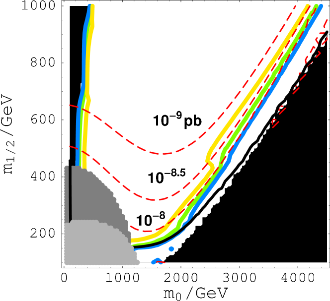
(b)

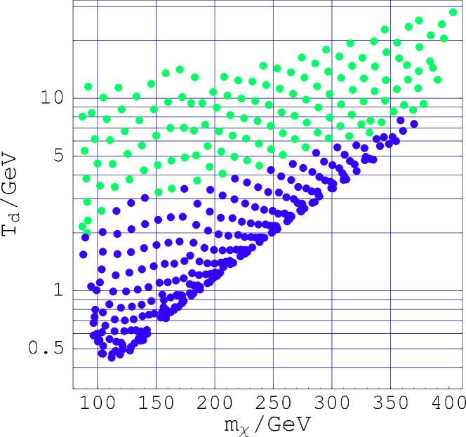
Figure 1: (a) The contours of $\Omega^{\rm th}_{\chi}h^{2}$ and $\sigma_{\chi-p}~{}[{\rm{pb}}]$. (b) The decay temperature of Q-ball which leads to the desired mass density of dark matter. ($\tan\beta=45$)

As we can see from Fig. 1-(a), $\Omega^{\rm th}_{\chi}h^{2}$ are too large to be consistent with the WMAP result, $\Omega_{DM}h^{2}=0.1126^{+0.0161}_{-0.0181}$, in most of the parameter space. However, as the parameter sets approach the “focus point” [33] region ($m_{0}\mathop{}_{\textstyle\sim}^{\textstyle>}$ TeV), the pair annihilation of neutralinos becomes more efficient because of the increase of Higgsino component in the LSP, and then, there appears a very thin parameter region that gives the correct abundance of the LSP [34].  As we further increase $m_{0}$, $\Omega^{\rm th}h^{2}$ continues to decline, and the late-time decay of Q-balls comes to be allowed to play an important role.

In Fig. 1-(b), we show the decay temperature of Q-ball in the ($m_{\chi}$, $T_{d}$) plane, which leads to the desired mass density of dark matter (see Eq. (22)). The light shaded (green) points denote the required $T_{d}$’s for $0.03\leq\Omega^{\rm th}_{\chi}h^{2}\leq 0.1$, and the dark shaded (blue) points for $\Omega^{\rm th}_{\chi}h^{2}<0.03$. This result suggests that the desirable parameter sets for the present scenario would give $\Omega^{\rm th}h^{2}<0.03$ in the thermal freeze-out scenario, since $T_{d}\leq{\cal O}(1)$ GeV is expected in the typical models of AD baryogenesis (Section 2). We can also see that the anticipated Q-ball decay temperature prefers the existence of a relatively light neutralino, $m_{\chi}\mathop{}_{\textstyle\sim}^{\textstyle<}300~{}{\rm GeV}$.

In the above calculation of the decay temperature, we have included only the $s$-wave contribution in the annihilation cross section of the neutralinos for the reasons explained before. We have also neglected the possible co-annihilation effects with the lightest charginos. This procedure can be justified as long as the decay temperature of the Q-ball is smaller than their mass difference $\delta m$. Actually, this condition is satisfied in almost the entire parameter space, where we have confirmed $\delta m={\cal O}(10)~{}{\rm GeV}$.

(a)

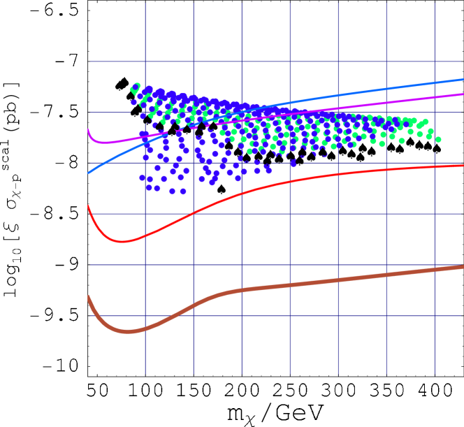
(b)

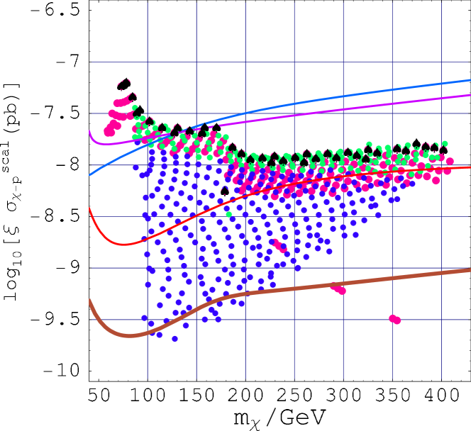
Figure 2: The effective cross section of proton-$\chi$ scalar interaction in the mSUGRA scenario. (a) The non-thermal scenario. (b) The standard thermal freeze-out scenario. ($\tan\beta=45$)

Now, let us turn our attention to the direct detection of the non-thermal dark matter. As one can see from Fig. 1-(a), the $\chi$-proton cross section $\sigma_{\chi-p}$ becomes larger as $m_{0}$ increases because of the increase of the Higgsino component in the LSP. Since the increase of Higgsino fraction reduces the relic density, we can expect larger direct detection rate in the non-thermal scenario. In Fig. 2, we show the effective $\chi$-proton cross section in the ($m_{\chi}$, $\xi\sigma_{\chi-p}$) plane in the mSUGRA scenario with $\tan\beta=45$. Fig. 2-(a) shows the cross section in the non-thermal scenario $(\xi=1)$, and Fig. 2-(b) shows it in the standard thermal scenario. In Fig. 2-(b) the cross section is rescaled by multiplying a factor $\xi=(\Omega^{\rm th}_{\chi}h^{2}/\Omega_{DM}h^{2})$ where $\Omega^{\rm th}_{\chi}h^{2}$ is smaller than $\Omega_{DM}h^{2}$, since the detection rate is proportional to the local neutralino density. 

The dark shaded (blue) points in the both figures correspond to the mSUGRA parameters with $\Omega^{\rm th}_{\chi}h^{2}\leq 0.03$, the light shaded (green) points to those with $0.03\leq\Omega^{\rm th}_{\chi}h^{2}\leq 0.1$ and the medium shaded (purple) points to those with $0.1\leq\Omega^{\rm th}_{\chi}h^{2}\leq 0.3$. We also plot the parameter sets which are consistent with the WMAP experiment ($\Omega^{\rm th}_{\chi}h^{2}=0.1126^{+0.0161}_{-0.0181}$) in the standard thermal scenario as black “$\spadesuit$” points,  which are also plotted in Fig. 2-(a) just for convenience to comparison. The four lines denote sensitivities of several direct detection experiments: ZEPLIN MAX [35], GENIUS [36], EDELWEISS II [37], and CDMS (Soudan) [38] from the bottom up, respectively. In Figs. 3 and 4, we also show the corresponding figures for $\tan\beta=10$ in the mSUGRA model, where conventions are the same as in Figs. 1 and 2.

In the above calculations, we have adopted the following values of the proton matrix elements for each of the three light quarks:

$$f_{T_{u}}=0.019,\,\,f_{T_{d}}=0.041,\,\,f_{T_{s}}=0.14,$$ (28)

where $f_{T_{q}}\equiv\langle p|m_{q}q\bar{q}|p\rangle/m_{p}$. For details about the calculation of the proton-$\chi$ cross section, see Refs. [27, 26].

(a)

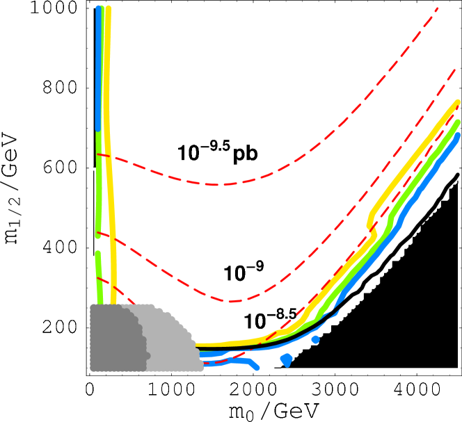
(b)

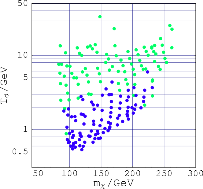
Figure 3: (a) The contours of $\Omega^{\rm th}_{\chi}h^{2}$ and $\sigma_{\chi-p}~{}[\rm{pb}]$. (b) The decay temperature of Q-ball which leads to the desired mass density of dark matter. ($\tan\beta=10$)

(a)

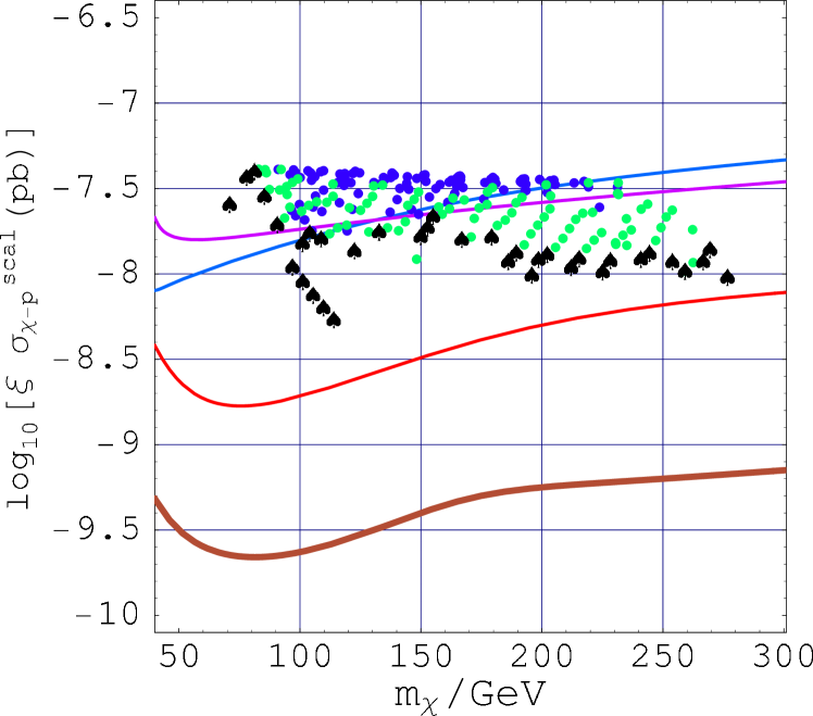
(b)

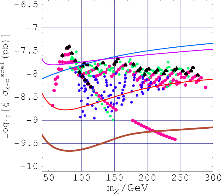
Figure 4: The effective cross section of proton-$\chi$ interaction in the mSUGRA scenario. (a) The non-thermal scenario. (b) The standard thermal freeze-out scenario. ($\tan\beta=10$)

From Figs. 2 and 4, we can see a clear difference between the thermal and non-thermal scenarios. First of all, the detection rates in the non-thermal scenario are larger than those in the standard scenario, denoted by $\spadesuit$ points, by several times, and most of the parameter space can be thoroughly surveyed by next generation detectors.  Secondly, since the preferred parameter sets for AD baryogenesis predict quite small relic densities in the thermal freeze-out scenario, the detection rates for the corresponding points in the standard scenario become much smaller than in the non-thermal scenario. This may play a crucial role to reveal the true thermal history of our Universe in the future.

4.1.2 Parameter space and direct detection in the mAMSB

Anomaly-mediated SUSY breaking (AMSB) [14] is another interesting way to mediate SUSY-breaking effects to the MSSM sector without conflicting with the well known FCNC problem. In the pure AMSB model, all the soft SUSY-breaking parameters are fully determined by $\beta$ functions of gauge and Yukawa coupling constants, and anomalous dimensions of matter fields. Quite unfortunately, however, the pure AMSB model predicts negative slepton masses, and hence is not capable of describing the real world.

Although many possible solutions have been proposed to this problem, we adopt the simplest solution in the present paper. We just assume the additional universal scalar mass $m_{0}$ at the GUT scale, and then evolve the RG equations to obtain the low-energy spectrum. In this minimal framework (mAMSB), the entire parameter space is specified by the following $4$ parameters:

$$m_{3/2},\,\,m_{0},\,\,\tan\beta,\,\,{\rm sgn(\mu)}.$$ (29)

In this model, the gaugino masses are not modified and almost the same as those in the pure AMSB model except higher oder quantum corrections. Their ratios at the weak scale are approximately give by

$$M_{1}\;:\;M_{2}\;:\;M_{3}\;\approx\;2.8\;:\;1\;:\;-8.3\;,$$ (30)

and the Wino-like LSP is realized in almost the entire parameter space. This fact has an important impact on the cosmology in the mAMSB model.

(a)

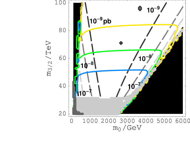
(b)

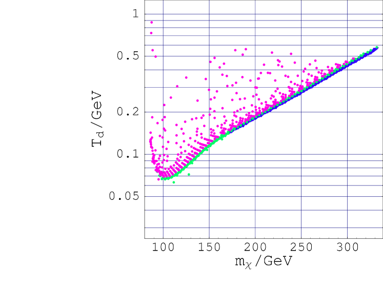
Figure 5: (a) The contours of $\Omega^{\rm th}_{\chi}h^{2}$ and $\sigma_{\chi-p}~{}[{\rm pb}]$. (b) The decay temperature of Q-ball which leads to the desired mass density of dark matter. ($\tan\beta=30$)

In Fig. 5-(a), we show contours of the relic neutralino density in the thermal freeze-out scenario and the $\chi$-proton scalar cross section for the case of $\tan\beta=30$ in the ($m_{0}$, $m_{3/2}$) plane. The horizontal lines correspond to the contours of the relic density, with $\Omega^{\rm th}_{\chi}h^{2}=10^{-3.2}$, $10^{-3.0}$ and $10^{-2.8}$, from the bottom up, respectively. Here, we have taken sgn($\mu$) negative to avoid too large contribution to the branching ratio of $b\to s\gamma$. The dashed lines are contours of the $\chi$-proton scalar cross section $\sigma_{\chi-p}$ whose value is explicitly denoted in the figure. The light shaded region is excluded by the chargino mass limit [40]. The lightest Higgs boson is lighter than 114 GeV in the dark shaded region. The black shaded region denotes the region where the electroweak symmetry breaking cannot be implemented, or the lightest stau or sneutrino becomes the LSP.

As we can see from Fig. 5-(a), $\Omega^{\rm th}_{\chi}h^{2}$ is much smaller than the required abundance of the LSP because of the large annihilation cross section of the Wino-like LSP in most of the parameter space. Therefore, in anyway, we need some non-standard thermal history to explain the required mass density of dark matter in this model, if we insist on the LSP as a primary component of the cold dark matter. The most natural answer to this problem is given by Affleck–Dine baryogenesis. If we use this mechanism to explain the observed baryon asymmetry, the associated late-time Q-ball decays with typical decay temperature $T_{d}\mathop{}_{\textstyle\sim}^{\textstyle<}{\cal{O}}(1)~{}{\rm GeV}$ can naturally generate the required abundance of the LSP at the same time [11, 13]. In fact, almost the entire parameter space of the mAMSB model is consistent with the Affleck–Dine baryo/DM-genesis scenario. 

In Fig. 5-(b), we show the decay temperature of Q-ball in the ($m_{\chi}$, $T_{d}$) plane, which leads to the required mass density. The dark shaded (blue) points correspond to the parameters with $Z_{H}\leq 0.01$, the light shaded points (green) to those with $0.01\leq Z_{H}\leq 0.03$ and the medium shaded (purple) to those with $0.03\leq Z_{H}$, where $Z_{H}$ is a Higgsino fraction in the LSP.  One can see that the required decay temperatures are about one magnitude smaller than those in the mSUGRA model, which comes from a larger annihilation cross section of the Wino-like LSP. As in the case of the mSUGRA model, we have included only the $s$-wave contributions in the annihilation cross section of the neutralino to calculate the decay temperature. We have also neglected the possible co-annihilation effects with the lightest charginos. In the mAMSB model, however, the mass splitting between the lightest chargino and neutralino is of the order of $100~{}{\rm MeV}\sim 1~{}{\rm GeV}$ [42], which has comparable size as $T_{d}$. Hence, the co-annihilation effects may slightly change the required decay temperature, which is at most a factor of few.

(a)

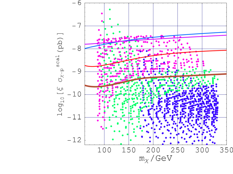
(b)

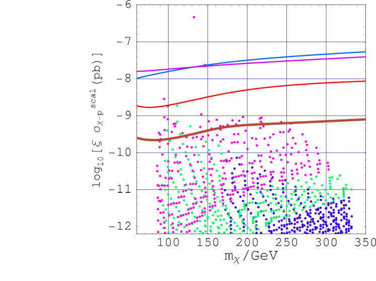
Figure 6: The effective cross section of proton-$\chi$ interaction in the mAMSB scenario. (a) The non-thermal scenario. (b) The standard thermal freeze-out scenario. $(\tan\beta=30)$

Now, let us discuss the direct detection rates in the mAMSB model. In Fig. 5-(a), there are two important factors to determine the $\chi$-proton cross section in this model. When the LSP is nearly pure Wino $(m_{0}\mathop{}_{\textstyle\sim}^{\textstyle<}2~{}{\rm TeV})$, the $\chi$-proton cross section is determined dominantly by the heavy Higgs exchange because of a large $\tan\beta$ enhancement. In this region, the shape of contours are controlled by the heavy Higgs boson mass $m_{H}$, and the $\chi$-proton cross section scales as $\sigma_{\chi-p}\propto 1/m_{H}^{4}$. As the parameter sets come close to the focus point region, the Higgsino component in the LSP becomes significant. In this region, the $\chi$-proton cross section is primarily determined by the light Higgs exchange, and the contours of $\sigma_{\chi-p}$ are controlled by the Higgsino fraction and have the same behavior seen in the mSUGRA model.

In Fig. 6, we show the effective $\chi$-proton cross section in the ($m_{\chi}$, $\xi\sigma_{\chi-p}$) plane for both the non-thermal (a) and the thermal freeze-out scenarios (b). The four lines are the sensitivities of several direct detection experiments explained in the previous section. Conventions of the shading (coloring) of the plotted points are the same as those in Fig. 5-(b): it shows the Higgsino fraction in the LSP. As in the mSUGRA model, we have set $\xi=1$ in the non-thermal scenario and $\xi=(\Omega_{\chi}^{\rm th}h^{2}/\Omega_{DM}h^{2})$ in the thermal scenario to obtain the effective $\chi$-proton cross section.

¿From the figures, in the non-thermal scenario, one can see that a large portion of the focus point region and the small $m_{H}$ region $(m_{0}\mathop{}_{\textstyle\sim}^{\textstyle<}1~{}{\rm TeV})$ are within the reach of next generation experiments. The bulk of the parameter space, where the Higgsino component of the LSP is very small and $m_{H}$ is large, is difficult to survey. In the case of the thermal freeze-out scenario, there is almost no hope to detect the signal of SUSY dark matter in the entire parameter space because of the smallness of the relic density of the LSP $(\xi\ll 1)$. In Figs. 7 and 8, we also show the corresponding figures for $\tan\beta=10$, where the conventions are the same as those in Figs. 5 and 6.

(a)

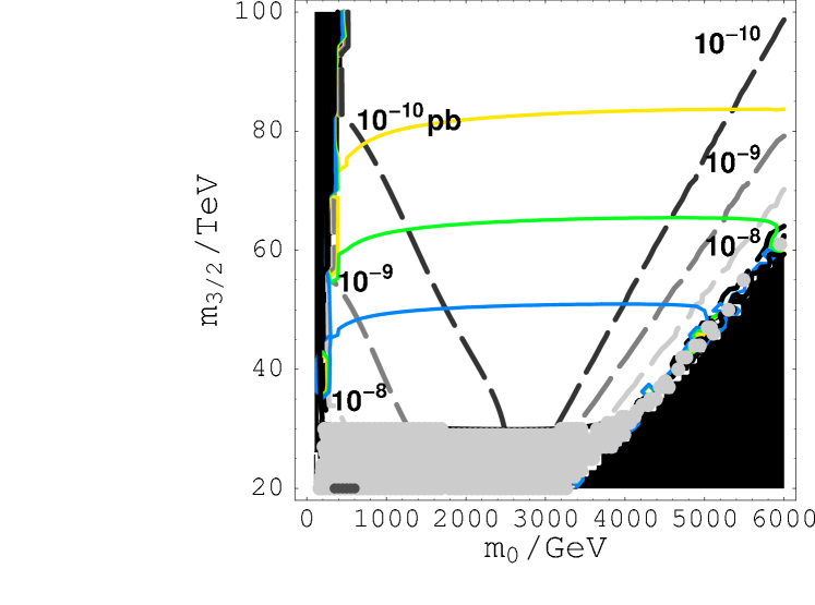
(b)

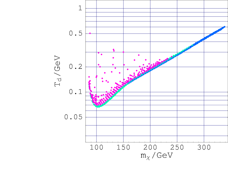
Figure 7: (a) The contours of $\Omega^{\rm th}_{\chi}h^{2}$ and $\sigma_{\chi-p}~{}[{\rm pb}]$. (b) The decay temperature of Q-ball which leads to the desired mass density of dark matter. ($\tan\beta=10$)

(a)

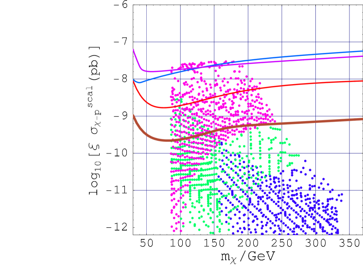
(b)

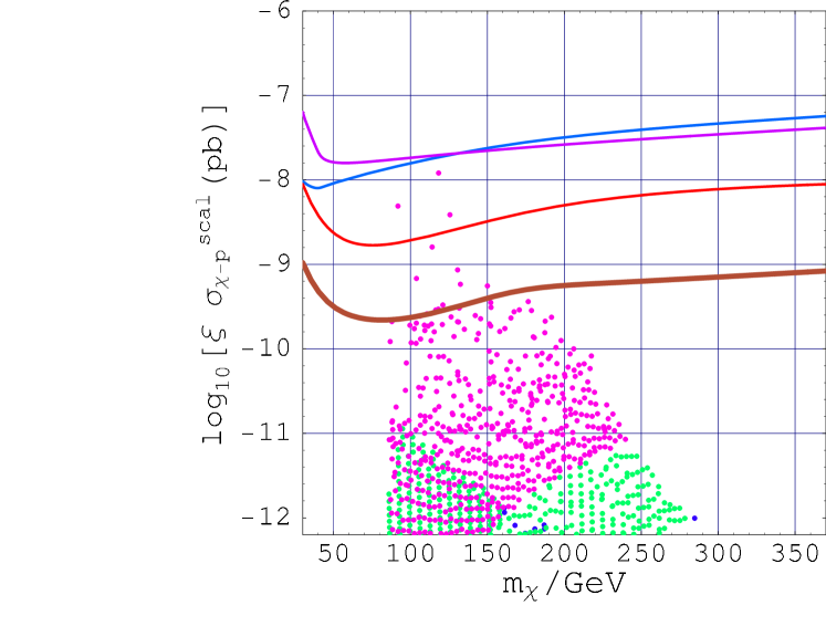
Figure 8: The effective cross section of proton-$\chi$ interaction in the mAMSB scenario. (a) The non-thermal scenario. (b) The standard thermal freeze-out scenario. $(\tan\beta=10)$

4.2 Indirect detection observing neutrino flux from the Sun

In this section, we discuss one of the most promising methods of indirect detection for the neutralino dark matter, which observes energetic neutrinos from annihilation of the LSP in the Sun. If the halo dark matter consists of the LSPs, the LSP has a finite possibility to be captured by the Sun by an elastic scattering with a nucleus therein. Once captured, the LSPs accumulate around the center of the Sun through additional scatterings with nuclei. Those LSPs which have accumulated in this way can annihilate with another LSP producing various decay products. Although most of them are immediately absorbed through interactions with surrounding matter to leave no evidence of their existence, produced neutrinos can escape out of the Sun and reach terrestrial detectors.

Especially, an energetic muon neutrino which escapes from the Sun and reaches the Earth, can be converted into a muon through a charged current interaction during passing through the rock below the detector. These muons induced from the energetic neutrinos can be detected by various astrophysical neutrino detectors installed deep under ground, sea water, or Antarctic ice. Since competing backgrounds are relatively well understood and also the nearby local halo density is constrained better than the entire halo profile, which is still highly controversial, we can make more definite predictions on the expected signal than they are in the cosmic-ray searches. In the rest of this section, we investigate the consequences of the Affleck–Dine baryo/DM-genesis scenario in this indirect detection method in the mSUGRA and mAMSB models, in turn.

4.2.1 Neutrino-induced muon flux from the Sun in the mSUGRA

First, let us discuss the prospects of the indirect detection of the neutrino-induced muon from the Sun in the mSUGRA model. The readers who are interested in a full detail of the required calculations, please consult the excellent review given in Ref. [26].

(a)

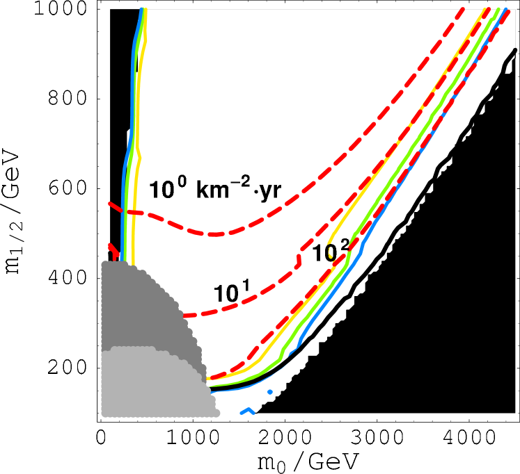
(b)

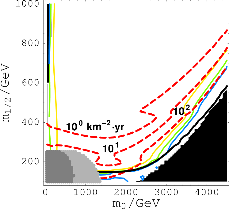
Figure 9: The $\mu$ flux from the Sun in the mSUGRA scenario. (a) $\tan\beta=45$. (b) $\tan\beta=10$. Here, the local neutralino density is fixed as $\rho_{\chi}=0.3~{}{\rm GeV}/{\rm cm}^{3}$.

In Fig. 9, we show the contours of the induced muon flux expected to be observed in a detector, where the dashed lines denote the expected flux and the other conventions are the same as those in Figs. 1 and 3. Note that, in this figure, the local neutralino density is fixed as $\rho_{\chi}=0.3~{}{\rm GeV}/{\rm cm}^{3}$ irrespective of the relic density, and hence, the actual detection rate in the thermal freeze-out scenario must be modified according to the value of $\Omega_{\chi}^{\rm th}h^{2}$.

Once we fix the local neutralino density, the size of the neutrino flux is primarily controlled by the neutralino capture rate of the Sun. Hence, the elastic scattering cross section between the LSP and nucleus in the Sun, not the annihilation cross section of the LSP, determines the resultant neutrino flux. Since the matter of the Sun largely consists of hydrogens, the spin-dependent interaction through the Z-boson exchange is the most important ingredient to determine the scattering cross section. The coupling to the Z-gauge boson is proportional to $N_{1,3(4)}^{2}$, and thus the flux becomes larger as Higgsino component in the LSP increases.

A large Higgsino fraction in the LSP has another advantage in this detection method. The detection probability for an energetic neutrino by observing the neutrino-induced upward muon is proportional to the second moment of the neutrino energy. This is because that both of the charged-current cross section and the range of the produced muon are roughly proportional to its energy. If the LSP has a significant fraction of Higgsino component, it can annihilate into a pair of W- or Z-gauge bosons with a large branching ratio. Since the subsequent decays of these gauge bosons produce the most energetic neutrinos, a large Higgsino component is very advantageous for the neutrino detection.

(a)

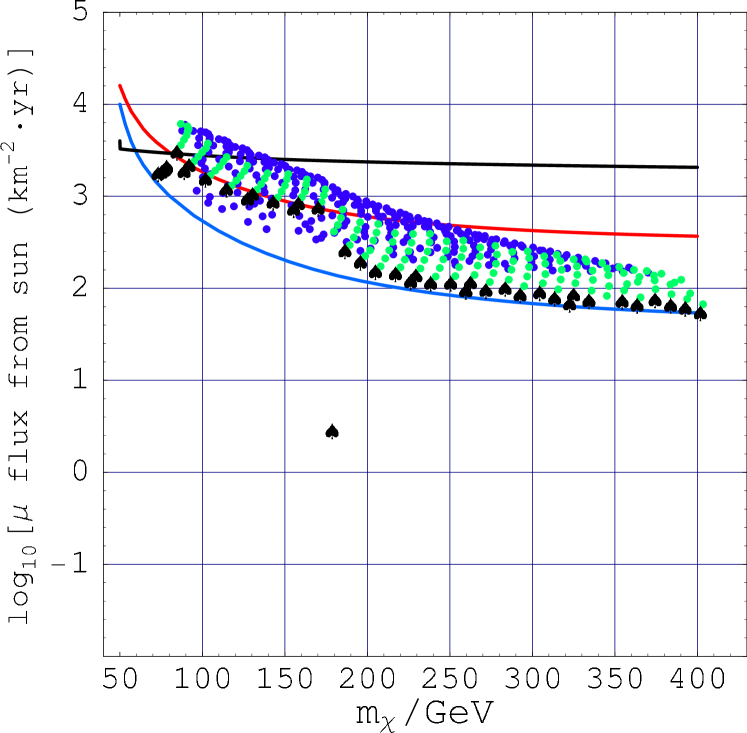
(b)

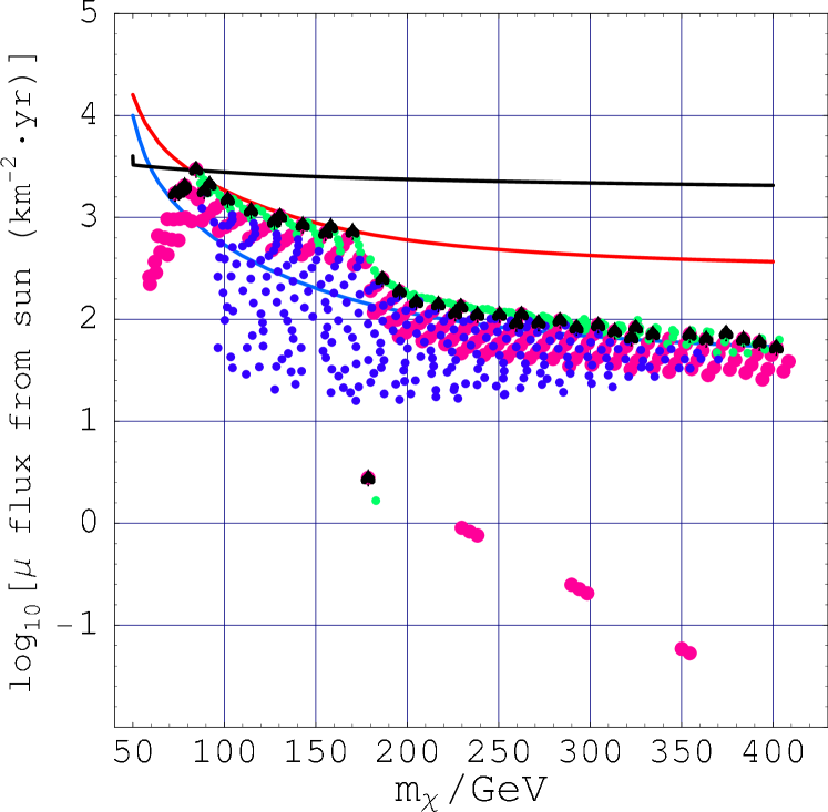
Figure 10: The $\mu$ flux from the Sun in the mSUGRA scenario. (a) The non-thermal scenario. (b) The standard thermal freeze-out scenario. ($\tan\beta=45$)

In Fig. 10, we show the expected $\mu$ flux from the Sun in the mSUGRA model with $\tan\beta=45$, in the non-thermal (a) and in the thermal freeze-out scenarios (b). Shading (coloring) conventions are the same as those in Fig. 2: dark (blue) points for $\Omega_{\chi}^{\rm th}h^{2}\leq 0.03$, light (green) points for $0.03\leq\Omega_{\chi}^{\rm th}h^{2}\leq 0.1$ and medium (purple) points for $0.1\leq\Omega_{\chi}^{\rm th}h^{2}\leq 0.3$. For the non-thermal scenario, we have calculated the expected muon flux with a fixed local neutralino density $\rho_{\chi}=0.3~{}{\rm GeV}/{\rm cm}^{3}$. As for the thermal freeze-out scenario, we have taken smallness of the local neutralino density into account by multiplying a factor $\xi=(\Omega_{\chi}^{\rm th}h^{2}/\Omega_{DM}h^{2})$ as before.  The black solid lines denote the present bound on the muon flux from Super Kamiokande [43]. The other two solid lines represent expected sensitivities for the muon flux in the near future experiments: ICECUBE [44] and ANTARES (3 years) [45] from the bottom up, respectively.

Fig. 10 clearly shows the advantage of the non-thermal scenario in the neutrino-induced muon detection. In the mSUGRA model, the late-time Q-ball decay requires a quite large annihilation cross section, which in turn, requires a significant fraction of Higgsino component in the LSP. This promises us a significant possibility to discover high-energy neutrino signals in the near future. Especially, for relative light neutralinos $m_{\chi}\mathop{}_{\textstyle\sim}^{\textstyle<}m_{t}$, there is a big possibility even for ANTARES, which is now in the last phase of its construction, to find the signals. Furthermore, after the deployment of the ICECUBE detectors, we can survey the whole parameter space of the non-thermal scenario. Similar features can be seen in Fig. 11, which is a corresponding figure for $\tan\beta=10$.

(a)

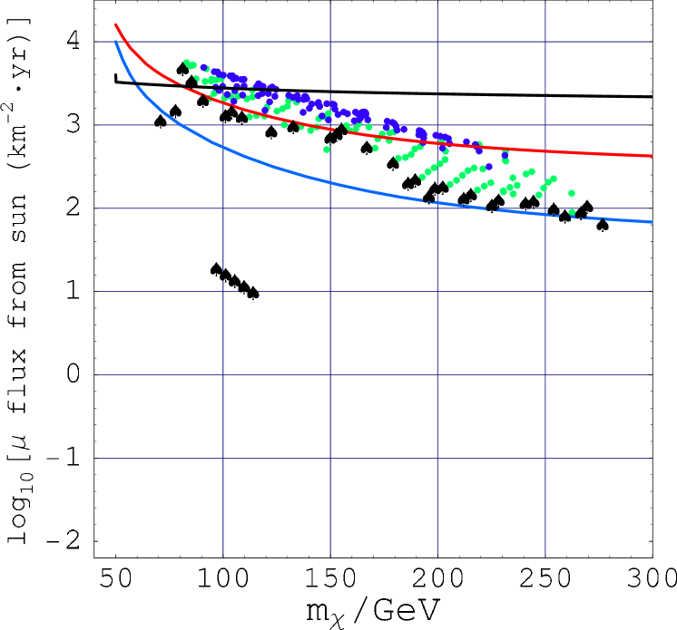
(b)

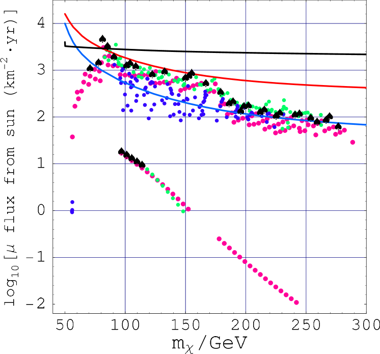
Figure 11: The $\mu$ flux from the Sun in the mSUGRA scenario. (a) The non-thermal scenario. (b) The standard thermal freeze-out scenario. ($\tan\beta=10$)

4.2.2 Neutrino-induced muon flux from the Sun in the mAMSB

Now, let turn our attention to the mAMSB model. Since the LSP in the mAMSB model is mostly composed of Wino, the spin-dependent (and also scalar) scattering cross section of the LSP with matter in the Sun is relatively small. This reduces the expected muon flux compared to the Higgsino-like dark matter.

(a)

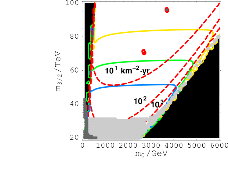
(b)

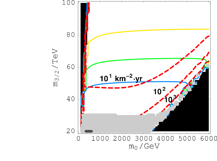
Figure 12: The $\mu$ flux from the Sun in the mAMSB scenario. (a) $\tan\beta=30$. (b) $\tan\beta=10$.

In Fig. 12, we show the contours of the expected muon flux in the mAMSB model with $\tan\beta=30$ (a) and $\tan\beta=10$ (b). The dashed lines denote the expected muon flux, whose value is explicitly presented in the figure. The other conventions are the same as those in Fig. 5-(a). As in the previous section, the local neutralino density is fixed as $\rho=0.3~{}{\rm GeV}/{\rm cm}^{3}$, and hence we need an adjustment in the thermal freeze-out scenario to obtain correct predictions. The muon flux increases as the parameter sets approach to the focus point region, where the LSP has a significant Higgsino fraction as in the mSUGRA case.

(a)

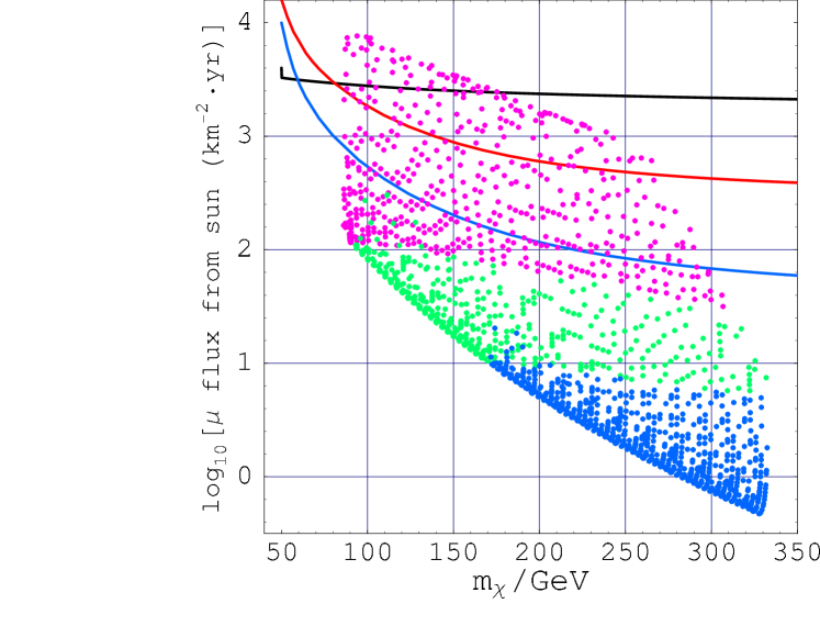
(b)

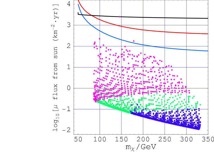
Figure 13: The $\mu$ flux from the Sun in the mAMSB scenario. (a) The non-thermal scenario. (b) The standard thermal freeze-out scenario. ($\tan\beta=30$)

(a)

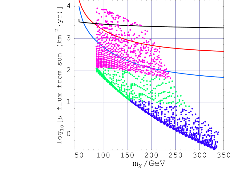
(b)

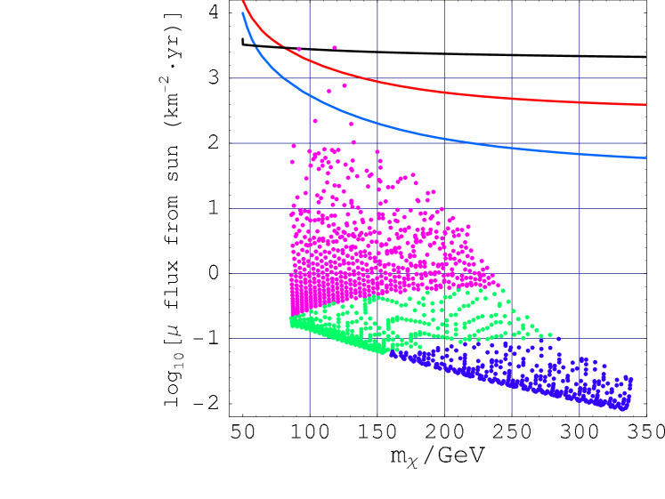
Figure 14: The $\mu$ flux from the Sun in the mAMSB scenario. (a) The non-thermal scenario. (b) The standard thermal freeze-out scenario. ($\tan\beta=10$)

Fig. 13 shows the expected muon flux for $(\tan\beta=30)$ in the non-thermal (a) and in the thermal freeze-out scenarios (b). For the non-thermal case, we have set the local neutralino density as $\rho_{\chi}=0.3~{}{\rm GeV}/{\rm cm}^{3}$, and for the thermal case, we have rescaled the flux by multiplying a factor $\xi=(\Omega_{\chi}^{\rm th}h^{2}/\Omega_{DM}h^{2})$ to take the smallness of the local neutralino density into account.  ¿From this figure, we can see that there is almost no chance to find energetic neutrino signals in the thermal freeze-out scenario, even after the completion of ICECUBE project. In other words, in the mAMSB model, it strongly indicates the existence of the non-thermal dark matter if we find energetic neutrino signals in the future experiments. We present the corresponding figure for $\tan\beta=10$ in Fig. 14.

4.3 Indirect detection observing hard positron flux from the halo

Finally, in this section, we discuss another promising way to indirectly detect the existence of neutralino dark matter: search for an excess of positron flux in cosmic rays in space based or balloon-borne experiments. At low energies, the expected positron flux has large uncertainty for lack of precise knowledge about competing backgrounds. Although the positron background is most likely to be composed of secondaries produced in the interactions of cosmic ray nuclei with interstellar gas, which is expected to fall as $\sim E_{e^{+}}^{-3.1}$, this background is suffering from large ambiguity coming from the solar wind at energies below $\sim 10~{}{\rm GeV}$ [46, 47]. It is also affected by the orbit path of the experiment. Fortunately, at high energies, these effects are strongly suppressed, and we can hope to have a meaningful signal. In addition, at high energies, the positrons lose their energy through various processes, and it is known that they can reach the detectors only when they are produced within a few $\rm kpc$ [46, 47]. Therefore, as for the hard positron spectrum, the result is rather insensitive relative to the controversial halo profile near the galactic center. 

The dominant source of the most energetic positron flux is the annihilation of two neutralinos into a $W^{\pm}$ or $Z^{0}$ pair, which is followed by the direct decay of the $W^{+}$ into an $e^{+}$ and $\nu_{e}$ or decay of the $Z^{0}$ into an $e^{\pm}$ pair.  The positrons produced as this way have an average energy of half the parent neutralino mass, and their spectrum has a peak around this energy, where the signal to background ratio is maximized.

We use the following result of the differential positron flux given in Ref. [47]:

$$E^{2}\frac{d\Phi_{e^{+}}}{d\Omega dE} = 2.7\times 10^{-6}{\rm cm}^{-2}{\rm s}^{-1}{\rm sr}^{-1}~{}{\rm GeV}$$ (32)

$$\times\left(\frac{\rho_{\chi}}{0.3~{}{\rm GeV}/{\rm cm}^{3}}\right)^{2}\left(\frac{100~{}{\rm GeV}}{m_{\chi}}\right)^{2}\sum_{i}\frac{\sigma_{i}v}{{\rm pb}\cdot\beta_{i}}B_{e^{+}}^{i}\int^{z^{i}_{+}}_{z^{i}_{-}}dz\;g(z,E/m_{\chi})\;,$$

where $i$ denotes an annihilation channel of the neutralinos into gauge bosons. The other required expressions are available in Refs. [47, 48]. Although we adopt the modified isothermal distribution with halo size $4{\rm kpc}$ as the halo profile, other choices do not change the main results for the reason explained before. We use $E^{2}d\Phi_{e^{+}}/d\Omega dE=1.16\times 10^{-3}E^{-1.23}$ as a fit of the positron background [48].

4.3.1 Hard positron flux in the mSUGRA

First, let us discuss the hard positron flux in the mSUGRA model. As discussed above, the hard positron flux is determined by the neutralino annihilation cross section into a pair of gauge bosons.

(a)

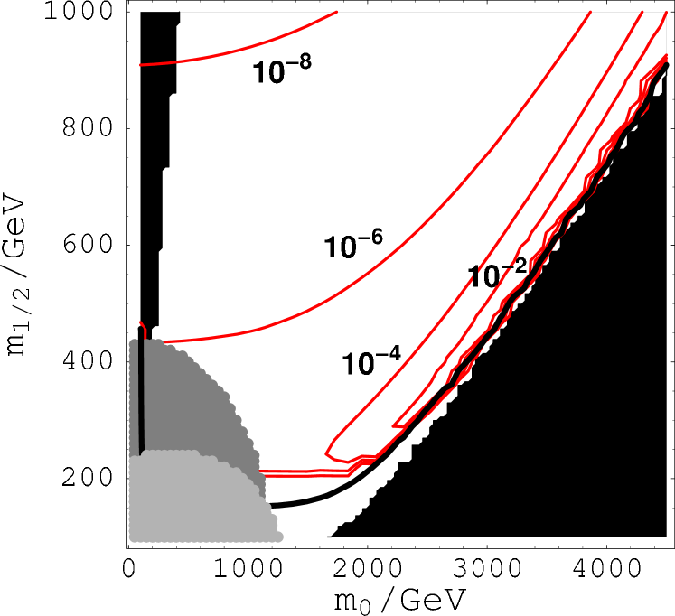
(b)

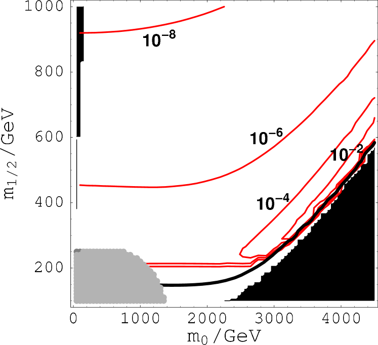
Figure 15: The positron signal to background ratio $S/B$ at $E_{\rm opt}$ in the mSUGRA scenario. (a) $\tan\beta=45$. (b) $\tan\beta=10$.

Therefore, we can expect that the flux increases as Higgsino component in the LSP increases, which makes the current non-thermal scenario much more advantageous than the standard thermal freeze-out scenario.

In Fig. 15, we show the contour plot of the positron signal to background ratio $S/B$ at $E_{\rm opt}$, where the $S/B$ is maximized. The solid (red) lines are the contours of $S/B$ whose value is denoted in the figure. Other conventions are the same as before. Note that, in this calculation, we have fixed the local neutralino density as $\rho_{\chi}=0.3~{}{\rm GeV}/{\rm cm}^{3}$ irrespective of the thermal relic abundance.

(a)

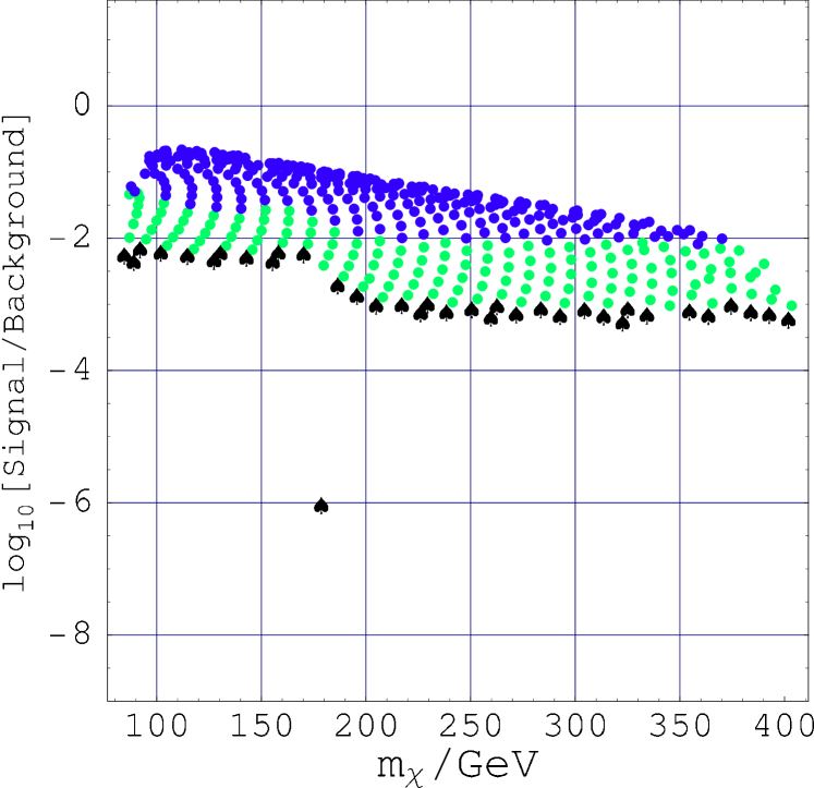
(b)

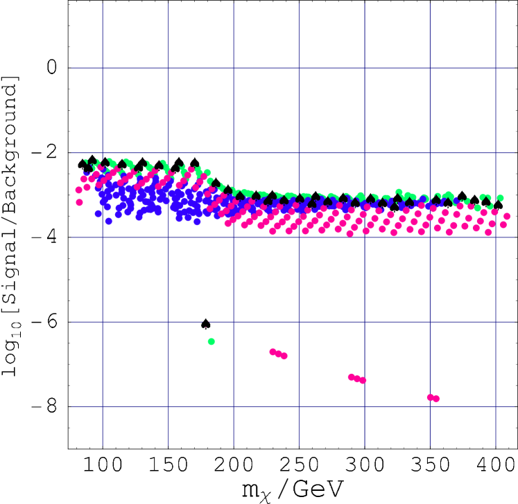
Figure 16: The positron signal to background ratio $S/B$ at $E_{\rm opt}$ in the mSUGRA scenario. (a) The non-thermal scenario. (b) The thermal freeze-out scenario. $(\tan\beta=45)$

In Fig. 16, we show the positron $S/B$ ratio in the non-thermal (a) and thermal freeze-out scenarios (b) in the mSUGRA model with $\tan\beta=45$. In the case of the non-thermal scenario, we have set the local neutralino density as $\rho_{\chi}=0.3~{}{\rm GeV}/{\rm cm}^{3}$, which means $\xi=1$. As for the thermal freeze-out scenario, we have rescaled the $S/B$ ratio by multiplying a factor $\xi^{2}=(\Omega_{\chi}^{\rm th}h^{2}/\Omega_{DM}h^{2})^{2}$ where $\Omega_{\chi}^{\rm th}h^{2}<\Omega_{DM}h^{2}$ so that we can take the size of the neutralino relic abundance into account. The shading (coloring) conventions are the same as those in Fig. 2: dark (blue) points denote the parameter sets that would lead to $\Omega_{\chi}^{\rm th}h^{2}\leq 0.03$ in the thermal scenario.

In the figure, the advantage of the non-thermal scenario is really distinctive. The preferred region for AD baryogenesis ($\Omega_{\chi}^{\rm th}h^{2}\leq 0.03$) provides quite large $S/B$ ratio, especially at the region $m_{\chi}\mathop{}_{\textstyle\sim}^{\textstyle<}m_{\rm top}$, where even $S/B\sim 10\%$ is possible. On the other hand, the thermal freeze-out scenario predicts very small $S/B$ ratio $<1\%$, particularly at the co-annihilation region. The expected sensitivity of the future space based experiments, such as AMS-$02$ [49], is roughly $\sim 1\%$. Therefore, although the estimation of the positron flux is suffering from various uncertainties, such as “clumpiness” of the local neutralino density, we can expect a good possibility to find a kind of “smoking-gun” signals of the non-thermal dark matter in the near future. In Fig. 17, we show the corresponding calculations for $\tan\beta=10$.

(a)

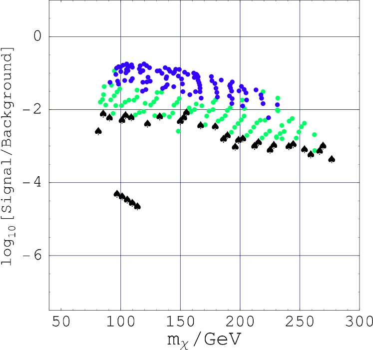
(b)

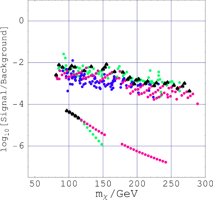
Figure 17: The positron signal to background ratio $S/B$ at $E_{\rm opt}$ in the mSUGRA scenario. (a) The non-thermal scenario. (b) The thermal freeze-out scenario. $(\tan\beta=10)$

4.3.2 Hard positron flux in the mAMSB

Now, let us discuss the expected positron flux in the mAMSB scenario. In this model, Wino-like LSP is realized in most of the parameter space, which has a larger annihilation cross section into gauge bosons than Higgsino-like LSP by roughly one order of magnitude. This fact allows us to have much more distinctive signals than those in the mSUGRA model, if the non-thermal DM-genesis had taken place in the early Universe. In Fig. 18, we show the contour plot of the positron signal to background ratio $S/B$ at $E_{\rm opt}$ with fixed local neutralino density as $\rho_{\chi}=0.3~{}{\rm GeV}/{\rm cm}^{3}$. In most of the allowed parameter region, $S/B\sim 1$ is expected.

(a)

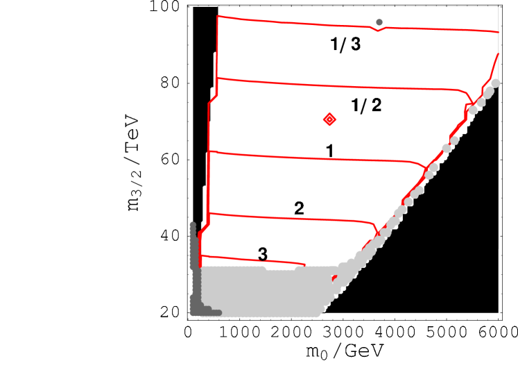
(b)

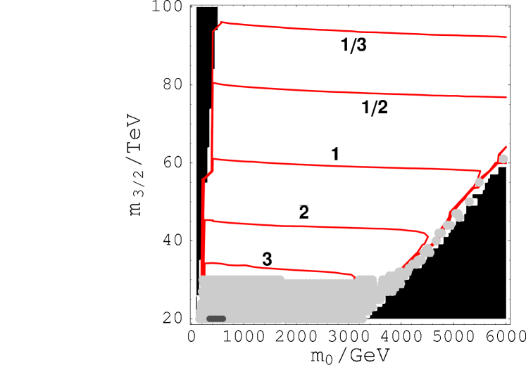
Figure 18: The positron signal to background ratio $S/B$ at $E_{\rm opt}$ in the mAMSB scenario. (a) $\tan\beta=30$. (b) $\tan\beta=10$.

(a)

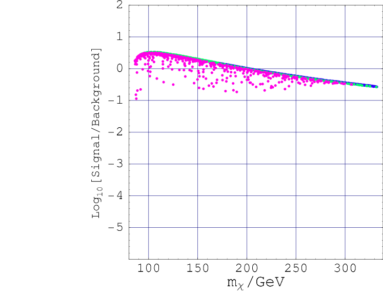
(b)

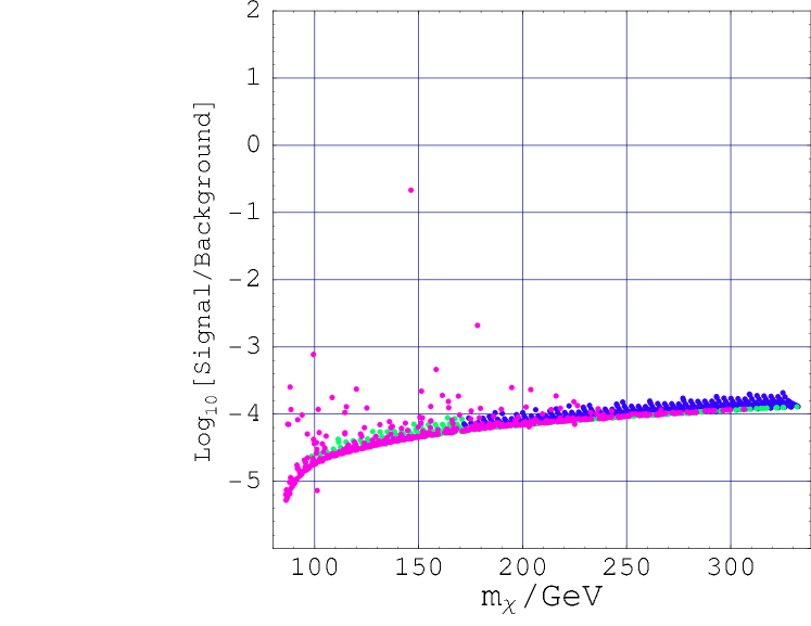
Figure 19: The positron signal to background ratio $S/B$ at $E_{\rm opt}$ in the mAMSB scenario. (a) The non-thermal scenario. (b) The thermal freeze-out scenario. $(\tan\beta=30)$

(a)

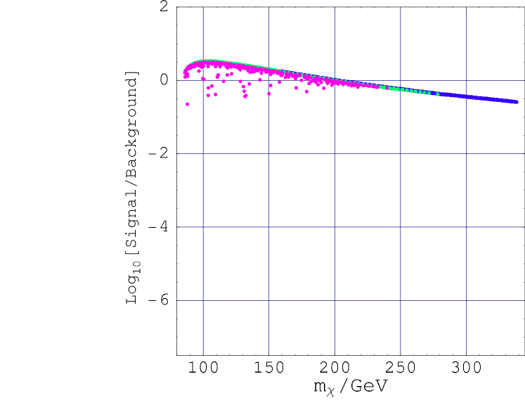
(b)

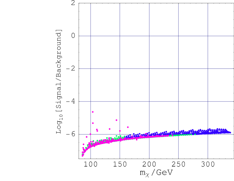
Figure 20: The positron signal to background ratio $S/B$ at $E_{\rm opt}$ in the mAMSB scenario. (a) The non-thermal scenario. (b) The thermal freeze-out scenario. $(\tan\beta=10)$

In Fig. 19, we present the signal to background ratio $S/B$ in the non-thermal (a) and the thermal freeze-out scenarios (b) for $\tan\beta=30$. The shading (coloring ) conventions are the same as those in Fig. 6, which denote the Higgsino fraction in the LSP. As in the case of the mSUGRA model, we have set $\xi=1$ in the non-thermal scenario, and rescaled the $S/B$ ratio by multiplying $\xi^{2}=(\Omega_{\chi}^{\rm th}h^{2}/\Omega_{DM}h^{2})^{2}$ in the thermal freeze-out scenario. As one can see, if the AD baryo/DM-genesis had really taken place in the early Universe, we will have really distinctive signals in the near future. On the other hand, in the thermal scenario, we cannot expect any observable signal because of smallness of the relic Wino density. Because we can survey only a limited parameter space in the mAMSB model by the direct detection and indirect dark matter search observing energetic neutrinos, the observation of the hard positron flux will play a crucial role to reveal the nature of dark matter in this model. In Fig. 20, we present a corresponding figure for $\tan\beta=10$.

5 Conclusions and discussion

In this paper, we have discussed the implications of the Affleck–Dine baryo/DM-genesis scenario in several ways of dark matter search. We have investigated two promising ways of indirect detection: one is the observation of the muon flux induced by the energetic neutrinos from the center of the Sun, and the other is to observe the hard positron flux from the halo. We have also updated the previous analysis of the direct detection by implementing the recent WMAP result to constrain the allowed parameter space, which allowed us to have more definitive predictions of the non-thermal scenario.

We have adopted the mSUGRA and mAMSB scenarios to demonstrate the predictions of the non-thermal scenario. In the mSUGRA model, Affleck–Dine baryogenesis prefers the “focus point” region to avoid overclosing the Universe, where the LSP contains non-negligible component of Higgsino. A large Higgsino fraction in the LSP increases all of the above mentioned detection rates, and we can survey the whole parameter space in the future experiments. Especially, for relatively light neutralinos $m_{\chi}\mathop{}_{\textstyle\sim}^{\textstyle<}m_{t}$, we have an intriguing possibility to discover dark matter signals in near future experiments, such as CDMS (Soudan) [38], EDELWEISS II [37] and ANTARES [45]. In the case of the mAMSB model, the thermal relic density is very small $\Omega_{\chi}^{\rm th}h^{2}\sim 10^{-3}$ in the entire parameter space, which makes the AD baryogenesis consistent in all over the region. Unfortunately, we can survey only a limited parameter space by the direct detection and indirect detection observing neutrino flux from the Sun. However, the quite large annihilation cross section into W-bosons promises us distinctive signals of the hard positron flux (and also of the mono-energetic photon from the direct annihilation channel: $\chi\chi\rightarrow\gamma\gamma/Z$) in the future experiments [50]. Although we have adopted the mSUGRA and mAMSB models for demonstration, since discussed detection rates are primarily determined by the Higgsino or Wino fraction in the LSP, we hope that the main predictions are not changed in other SUSY-breaking models.

Very encouragingly, though we have to wait father confirmations, there already exist some interesting experimental signals which can be naturally explained by Higgsino- or Wino-like non-thermal dark matter. The recent HEAT balloon experiment [51] has reported a significant excess of positrons in cosmic rays. The authors of Refs. [52, 53] have argued that a Higgsino or Wino LSP with mass $m_{W}<m_{\chi}\mathop{}_{\textstyle\sim}^{\textstyle<}200~{}{\rm GeV}$ could yield a consistent positron flux provided the relic abundance is from a non-thermal source. The EGRET [54] telescope has also identified a gamma-ray source at the galactic center. The authors of Ref. [55] have argued that the spectrum features of this source are compatible with the gamma-ray flux induced by pair annihilations of dark matter neutralinos. They have shown that the discrimination between this interesting interpretation and other viable explanations will be possible with GLAST [56], the next major gamma-ray telescope in space.

Finally, let us comment on the generality of the non-thermal dark matter. In the present work, we have assumed Affleck–Dine baryogenesis as the origin of the non-thermal source of the LSP. However, we think that the existence of the non-thermal dark matter is a much more generic prediction of the MSSM, or any kind of SUSY standard models. Once we assume MSSM-like models, we inevitably have many flat directions. Because we believe the existence of an inflationary era in the very beginning of the Universe, we have a good reason to expect that there are couplings between inflaton and SM fields in the Kähler potential in the following form:

$$\delta K=\frac{b}{M_{*}^{2}}I^{{\dagger}}I\Phi^{{\dagger}}\Phi\;,$$

where $I$ is the inflaton superfield and $\Phi$ denotes any kind of SM field. In order to ensure for all the flat directions to have positive Hubble-order mass term, we have to assume $b<1$ for arbitrary combinations of ${\Phi}$ along flat directions. 

This seems a rather strong assumption. We think that it is much more natural, or at least comparably natural, that some flat direction has a negative Hubble-order mass term and develops a large expectation value during the inflationary stage. This generally leads to the same non-thermal DM-genesis as discussed in this paper. There is no need for the flat direction to carry non-zero baryon number. If the flat direction is lifted by some non-renormalizable operator in the superpotential, the flat-direction field is likely not to dominate the energy density of the Universe, and hence it does not lead to an additional entropy production. In this case, we can make use of the standard leptogenesis to produce the observed baryon asymmetry. Note that the decay temperature of Q-balls is mainly determined by the initial amplitude of the flat-direction field, and hence, $T_{d}\mathop{}_{\textstyle\sim}^{\textstyle<}{\cal O}(1)~{}{\rm GeV}$ is a quite generic prediction.  These observations lead us to consider the Higgsino- or Wino-like non-thermal dark matter as a quite natural consequence of the MSSM or other SUSY standard models. We hope that this work will encourage serious research on the non-thermal dark matter by many researchers.

References

- [1] C. L. Bennett et al., arXiv:astro-ph/0302207; D. N. Spergel et al., arXiv:astro-ph/0302209; H. V. Peiris et al., arXiv:astro-ph/0302225.
- [2] M. Fukugita and T. Yanagida, Phys. Lett. B 174, 45 (1986).
- [3] For reviews and references, see, for example: M. Plumacher, Nucl. Phys. B 530, 207 (1998) [arXiv:hep-ph/9704231]; W. Buchmuller and M. Plumacher, Int. J. Mod. Phys. A 15, 5047 (2000) [arXiv:hep-ph/0007176]; W. Buchmuller, P. Di Bari and M. Plumacher, Nucl. Phys. B 643, 367 (2002) [arXiv:hep-ph/0205349].
- [4] G. Lazarides and Q. Shafi, Phys. Lett. B 258, 305 (1991); K. Kumekawa, T. Moroi and T. Yanagida, Prog. Theor. Phys. 92, 437 (1994) [arXiv:hep-ph/9405337]; G. Lazarides, in Symmetries in Intermediate and High Energy Physics, edited by A. Faessler, T. S. Kosmas, and G. K. Leontaris, Tracts in Modern Physics Vol. 163 (Springer, Berlin, 2000), p. 227, and references therein; G. F. Giudice, M. Peloso, A. Riotto and I. Tkachev, JHEP 9908, 014 (1999) [arXiv:hep-ph/9905242]; T. Asaka, K. Hamaguchi, M. Kawasaki and T. Yanagida, Phys. Lett. B 464, 12 (1999) [arXiv:hep-ph/9906366]; Phys. Rev. D 61, 083512 (2000) [arXiv:hep-ph/9907559]; K. Hamaguchi, H. Murayama and T. Yanagida, Phys. Rev. D 65, 043512 (2002) [arXiv:hep-ph/0109030]. M. Fujii, K. Hamaguchi and T. Yanagida, Phys. Rev. D 65, 115012 (2002) [arXiv:hep-ph/0202210].
- [5] I. Affleck and M. Dine, Nucl. Phys. B 249, 361 (1985).
- [6] For recent reviews, see, K. Enqvist and A. Mazumdar, Phys. Rept. 380, 99 (2003) [arXiv:hep-ph/0209244]; M. Dine and A. Kusenko, arXiv:hep-ph/0303065.
- [7] S. R. Coleman, Nucl. Phys. B 262, 263 (1985) [Erratum-ibid. B 269, 744 (1986)].
- [8] G. R. Dvali, A. Kusenko and M. E. Shaposhnikov, Phys. Lett. B 417, 99 (1998) [arXiv:hep-ph/9707423]; A. Kusenko and M. E. Shaposhnikov, Phys. Lett. B 418, 46 (1998) [arXiv:hep-ph/9709492].
- [9] K. Enqvist and J. McDonald, Phys. Lett. B 425, 309 (1998) [arXiv:hep-ph/9711514]; K. Enqvist and J. McDonald, Nucl. Phys. B 538, 321 (1999) [arXiv:hep-ph/9803380].
- [10] M. Fujii, K. Hamaguchi and T. Yanagida, Phys. Rev. D 64, 123526 (2001) [arXiv:hep-ph/0104186].
- [11] M. Fujii and K. Hamaguchi, Phys. Lett. B 525, 143 (2002) [arXiv:hep-ph/0110072].
- [12] M. Fujii and T. Yanagida, Phys. Lett. B 542 (2002) 80 [arXiv:hep-ph/0206066].
- [13] M. Fujii and K. Hamaguchi, Phys. Rev. D 66 (2002) 083501 [arXiv:hep-ph/0205044].
- [14] L. Randall and R. Sundrum, Nucl. Phys. B 557, 79 (1999) [arXiv:hep-th/9810155]; G. F. Giudice, M. A. Luty, H. Murayama and R. Rattazzi, JHEP 9812, 027 (1998) [arXiv:hep-ph/9810442].
- [15] L. Bergstrom and P. Ullio, Nucl. Phys. B 504, 27 (1997) [arXiv:hep-ph/9706232]; L. Bergstrom, P. Ullio and J. H. Buckley, Astropart. Phys. 9, 137 (1998) [arXiv:astro-ph/9712318]; see also recent developments, P. Ullio, L. Bergstrom, J. Edsjo and C. Lacey, Phys. Rev. D 66, 123502 (2002) [arXiv:astro-ph/0207125]; J. Hisano, S. Matsumoto and M. M. Nojiri, Phys. Rev. D 67, 075014 (2003) [arXiv:hep-ph/0212022]; J. Hisano, S. Matsumoto and M. M. Nojiri, arXiv:hep-ph/0307216.
- [16] G. Belanger, F. Boudjema, A. Pukhov and A. Semenov, Comput. Phys. Commun. 149, 103 (2002) [arXiv:hep-ph/0112278].
- [17] H. Murayama and T. Yanagida, Phys. Lett. B 322, 349 (1994) [arXiv:hep-ph/9310297]; T. Moroi and H. Murayama, JHEP 0007, 009 (2000) [arXiv:hep-ph/9908223].
- [18] T. Asaka, M. Fujii, K. Hamaguchi and T. Yanagida, Phys. Rev. D 62, 123514 (2000) [arXiv:hep-ph/0008041]; M. Fujii, K. Hamaguchi and T. Yanagida, Phys. Rev. D 63, 123513 (2001) [arXiv:hep-ph/0102187]; M. Fujii, K. Hamaguchi and T. Yanagida, Phys. Rev. D 65, 043511 (2002) [arXiv:hep-ph/0109154]; R. Allahverdi, M. Drees and A. Mazumdar, Phys. Rev. D 65, 065010 (2002) [arXiv:hep-ph/0110136]; M. Fujii, K. Hamaguchi and T. Yanagida, Phys. Lett. B 538, 107 (2002) [arXiv:hep-ph/0203189];
- [19] T. Gherghetta, C. F. Kolda and S. P. Martin, Nucl. Phys. B 468, 37 (1996) [arXiv:hep-ph/9510370].
- [20] M. Dine, L. Randall and S. Thomas, Phys. Rev. Lett. 75, 398 (1995) [arXiv:hep-ph/9503303]; M. Dine, L. Randall and S. Thomas, Nucl. Phys. B 458, 291 (1996) [arXiv:hep-ph/9507453].
- [21] N. Sakai and T. Yanagida, Nucl. Phys. B 197, 533 (1982); S. Weinberg, Phys. Rev. D 26, 287 (1982).
- [22] J. Hisano, H. Murayama and T. Yanagida, Nucl. Phys. B 402, 46 (1993) [arXiv:hep-ph/9207279]; T. Goto and T. Nihei, Phys. Rev. D 59, 115009 (1999) [arXiv:hep-ph/9808255]; H. Murayama and A. Pierce, Phys. Rev. D 65, 055009 (2002) [arXiv:hep-ph/0108104].
- [23] S. Kasuya and M. Kawasaki, Phys. Rev. D 62, 023512 (2000) [arXiv:hep-ph/0002285]; Phys. Rev. D 64, 123515 (2001) [arXiv:hep-ph/0106119].
- [24] A. G. Cohen, S. R. Coleman, H. Georgi and A. Manohar, Nucl. Phys. B 272, 301 (1986).
- [25] V. A. Bednyakov, H. V. Klapdor-Kleingrothaus and S. Kovalenko, Phys. Rev. D 50, 7128 (1994) [arXiv:hep-ph/9401262].
- [26] G. Jungman, M. Kamionkowski and K. Griest, Phys. Rept. 267, 195 (1996) [arXiv:hep-ph/9506380].
- [27] M. Drees and M. Nojiri, Phys. Rev. D 48, 3483 (1993) [arXiv:hep-ph/9307208].
- [28] B. C. Allanach, Comput. Phys. Commun. 143, 305 (2002) [arXiv:hep-ph/0104145].
- [29] D. M. Pierce, J. A. Bagger, K. T. Matchev and R. j. Zhang, Nucl. Phys. B 491, 3 (1997) [arXiv:hep-ph/9606211].
- [30] K. Hagiwara et al. [Particle Data Group Collaboration], Phys. Rev. D 66, 010001 (2002).
- [31] Joint LEP 2 Supersymmetry Working Group, Combined LEP Chargino Results, up to GeV, http://lepsusy.web.cern.ch/lepsusy/www/inos_moriond01/charginos_pub.html.
- [32] LEP Higgs Working Group for Higgs boson searches, OPAL Collaboration, ALEPH Collaboration, DELPHI Collaboration and L3 Collaboration, Search for the Standard Model Higgs Boson at LEP, CERN-EP/2003-011, available from http://lephiggs.web.cern.ch/LEPHIGGS/papers/index.html.
- [33] J. L. Feng, K. T. Matchev and T. Moroi, Phys. Rev. Lett. 84, 2322 (2000) [arXiv:hep-ph/9908309]; Phys. Rev. D 61, 075005 (2000) [arXiv:hep-ph/9909334].
- [34] J. L. Feng, K. T. Matchev and F. Wilczek, Phys. Lett. B 482, 388 (2000) [arXiv:hep-ph/0004043].
- [35] D. B. Cline, arXiv:astro-ph/0111098; D. B. Cline, H. g. Wang and Y. Seo, in Proc. of the APS/DPF/DPB Summer Study on the Future of Particle Physics (Snowmass 2001) ed. N. Graf, eConf C010630, E108 (2001) [arXiv:astro-ph/0108147].
- [36] H. V. Klapdor-Kleingrothaus et al. [GENIUS Collaboration], arXiv:hep-ph/9910205.
- [37] V. Sanglard [the EDELWEISS Collaboration], arXiv:astro-ph/0306233.
- [38] D. Abrams et al. [CDMS Collaboration], Phys. Rev. D 66, 122003 (2002) [arXiv:astro-ph/0203500]; http://cdms.berkeley.edu/
- [39] M. Drees, M. M. Nojiri, D. P. Roy and Y. Yamada, Phys. Rev. D 56, 276 (1997) [Erratum-ibid. D 64, 039901 (2001)] [arXiv:hep-ph/9701219].
- [40] A. Heister et al. [ALEPH Collaboration], Phys. Lett. B 533, 223 (2002) [arXiv:hep-ex/0203020].
- [41] T. Moroi and L. Randall, Nucl. Phys. B 570, 455 (2000) [arXiv:hep-ph/9906527].
- [42] T. Gherghetta, G. F. Giudice and J. D. Wells, Nucl. Phys. B 559, 27 (1999) [arXiv:hep-ph/9904378]; J. L. Feng, T. Moroi, L. Randall, M. Strassler and S. f. Su, Phys. Rev. Lett. 83, 1731 (1999) [arXiv:hep-ph/9904250].
- [43] A. Habig [Super-Kamiokande Collaboration], arXiv:hep-ex/0106024.
-
[44]
J. Edsjo. Swedish astroparticle physics, talk given at the conference
‘partikeldagarna’,uppala, sweden, march 6. 2001;
L. Bergstrom, J. Edsjo and P. Gondolo,
Phys. Rev. D 58, 103519 (1998)
[arXiv:hep-ph/9806293].
http://icecube.wisc.edu/ -
[45]
L. Thompson. Dark matter prospects with the antares neutrino telescope,
talk given atthe conference dark 2002, cape town, south africa 4-9
feb.2002.
http://antares.in2p3.fr/index.html - [46] E. A. Baltz and J. Edsjo, Phys. Rev. D 59, 023511 (1999) [arXiv:astro-ph/9808243].
- [47] I. V. Moskalenko and A. W. Strong, Phys. Rev. D 60, 063003 (1999) [arXiv:astro-ph/9905283].
- [48] J. L. Feng, K. T. Matchev and F. Wilczek, Phys. Rev. D 63, 045024 (2001) [arXiv:astro-ph/0008115].
- [49] S. P. Ahlen et al., Nucl. Instrum. Meth. A 350, 351 (1994); J. Alcaraz et al. [AMS Collaboration], Nucl. Instrum. Meth. A 478, 119 (2002); http://ams.cern.ch/
- [50] P. Ullio, JHEP 0106, 053 (2001) [arXiv:hep-ph/0105052].
- [51] S. W. Barwick et al. [HEAT Collaboration], Astrophys. J. 482, L191 (1997) [arXiv:astro-ph/9703192]; S. Coutu et al., Astropart. Phys. 11, 429 (1999) [arXiv:astro-ph/9902162]; S. Coutu et al., “Positron measurements with the HEAT-pbar instrument,” Proceedings of ICRC 2001.
- [52] G. L. Kane, L. T. Wang and J. D. Wells, Phys. Rev. D 65, 057701 (2002) [arXiv:hep-ph/0108138];
- [53] G. L. Kane, L. T. Wang and T. T. Wang, Phys. Lett. B 536, 263 (2002) [arXiv:hep-ph/0202156].
- [54] H. Mayer-Hasselwander et al., Astron. Astrophys. 335 (1998) 161.
- [55] A. Cesarini, F. Fucito, A. Lionetto, A. Morselli and P. Ullio, arXiv:astro-ph/0305075.
- [56] Proposal for the Gamma-ray Large Area Space Telescope, SLAC-R-522 (1998); GLAST Proposal to NASA A0-99-055-03 (1999).