TPJU-5/2003 Pentaquark in the Skyrme Model

Abstract

The mass of the newly discovered pentaquark is calculated within the framework of the SU(3) Skyrme Model. Various estimates based on the model independent approach are compared with the model results and with the Chiral Quark Model. Our discussion shows that $\Theta^{+}$ is light with the mass of the order 1.5 GeV.

1. Introduction

It seems that the new exotic spin $1/2$ baryon of strangeness $+1$, $\Theta^{+}$, is now well established experimentally [1],[2],[3],[4]. After the first report by Nakano, three other experiments have already confirmed the existence of $\Theta^{+}$ with mass $M_{\Theta^{+}}\simeq 1540$ MeV and very small width $\Gamma_{\Theta^{+}}<25$ MeV. It is interesting to note that such a state was predicted in the late 80-ies within the framework of the Skyrme Model. Indeed, Manohar [5] and Chemtob in Ref.[6] mentioned that the SU(3) Skyrme Model [7],[8],[9] (SM) not only reproduced the spectrum of the lowest baryon multiplets $8$ and $10$, but also predicted the new, exotic states belonging to the higher SU(3) representations like $\overline{10}$ or $27$. Such states were also seen in the KN scattering phase shifts calculated within SM in Refs.[10],[11]. In 1987 in Ref.[12] we presented the first estimate of the mass of the lightest member of $\overline{10}$ – today’s $\Theta^{+}$ – with the result $M_{\Theta^{+}}\simeq 1530$ MeV; in a striking agreement with the present experimental observations. Since the details of this estimate were never published, we think that it is worthwhile to recall shortly how this result was actually obtained.

The real boost in this field was due to Ref.[13] published in 1997, where not only the mass of $\Theta^{+}$ but also its width was calculated within the framework of the Chiral Quark Model ($\chi$QM) [14]. In fact both SM and $\chi$QM have similar group theoretical structure and the main problem in both models consisted in estimating the average mass of the exotic antidecuplet, $M_{\overline{10}}$. The splittings within $\overline{10}$ are to a good approximation in the first order in the symmetry breaker, $m_{s}$, identical as in the usual decuplet, i.e. proportional to the hypercharge $Y$, with proportionality coefficient being of the order of $150$ MeV. The problem of fixing $M_{\overline{10}}$ was solved in Ref.[13] by the assumption that the nucleon resonance N${}^{\ast}(1710)$ belongs to $\overline{10}$. An immediate consequence of this assignment was that $M_{\Theta^{+}}\simeq M_{N^{\ast}}-150=1560$ MeV. A more refined analysis of the antidecuplet splittings pushed the $\Theta^{+}$ mass further down to the value of 1530 MeV [13].

In our old estimate of the $\Theta^{+}$ mass [12] we used the second order perturbation theory in the strange quark mass $m_{s}$. This allowed us to estimate the strange moment of inertia of the rotating soliton which is responsible for the $\overline{10}-8$ mass splitting. Therefore our analysis did not rely on any physical assumption assigning some existing nucleon resonance to $\overline{10}$. The price, however, was that the mass of $\Theta^{+}$ depended rather strongly on the value of $m_{s}$ and/or pion nucleon $\Sigma_{\pi N}$ term.

2. Baryons in the chiral models

Chiral models like $\chi$QM or SM are closely related to QCD [14]. One can formally integrate out gluons from the QCD Lagrangian, then the resulting nonlocal quark theory would necessarily respect chiral symmetry. One can approximate this complicated theory by a simple, chirally symmetric, quartic quark interactions. A model with such properties was formulated by Nambu and Jona-Lasinio [15], however in a different context. NJL model exhibits an important phenomenon: spontaneous chiral symmetry breaking. As a result massless quark-antiquark bound states emerge – pions, kaons and $\eta$ ($\varphi_{a}$ in short). Formally, one can now reexpress the interaction part of the NJL Lagrangian introducing auxiliary, composite meson fields. This is the Chiral Quark Model used in Ref.[13] and derived from QCD within the instanon model of the QCD vacuum [16].

Notice the absence of the explicit meson kinetic energy and meson self-interaction terms in $\chi$QM: they arise only from the quark loops when one integrates out the quark fields. The resulting Lagrangian can be organized in terms of a number of derivatives of the meson fields (gradient expansion) [17]. A simple Ansatz for such a Lagrangian density was proposed by Skyrme 40 years ago [18]:

$$\mathcal{L}=\frac{F_{\pi}^{2}}{16}\operatorname*{Tr}\left(\partial_{\mu}U^{\dagger}\partial^{\mu}U\right)+\frac{1}{32e^{2}}\operatorname*{Tr}\left(\left[\partial_{\mu}U\,U^{\dagger},\partial_{\nu}U\,U^{\dagger}\right]^{2}\right)+\Gamma_{\text{WZ}}.$$ (1)

Here $U=\exp\left(i2\varphi_{a}\lambda_{a}/F_{\pi}\right)$, $F_{\pi}=186$ MeV, $e$ denotes the Skyrme parameter of the order $4-5$ and $\Gamma_{\text{WZ}}$ stands for the Wess-Zumiono term [19],[20].

Clearly, both $\chi$QM and SM are devised to describe meson physics at low energies. However, as realized by Skyrme [18] and later by Witten [20] and collaborators [21], there exists a solitonic solution – a nontrivial classical configuration of the meson fields, taken in the form of the hedgehog Ansatz:

$$U_{0}=\left[\begin{array}[c]{cc}e^{i\vec{n}\cdot\vec{\tau}\,P(r)}&0\\ 0&1\end{array}\right]$$ (2)

– which can be interpreted as a baryon. Further quantization of the rotational zero modes (both in the configuration space and in the flavor space), i.e. rotations of the meson fields $U=AU_{0}A^{\dagger}$ parameterized by a time dependent SU(3) matrix $A(t)$, provides quantum numbers corresponding to the different baryonic states [7],[8],[9]. In the chiral symmetry limit the effective baryonic Hamiltonian takes the following form:

$$H_{0}=M_{\text{cl}}+\frac{1}{2I_{1}}S(S+1)+\frac{1}{2I_{2}}\left(C_{2}(\mathcal{R})-S(S+1)-\frac{N_{{c}}^{2}}{12}\right).$$ (3)

Here $S$ denotes baryon spin, $C_{2}(\mathcal{R})$ the Casimir operator for the SU(3) representation $\mathcal{R}=(p,q)$:

$$C_{2}(\mathcal{R})=\frac{1}{3}\left(p^{2}+q^{2}+pq+3(p+q)\right).$$ (4)

The classical soliton mass $M_{\text{cl}}[P]$, and two moments of inertia $I_{1,2}[P]$ are functionals of the solitonic solution (2) and can be numerically calculated within the model considered. However, as already observed in Ref.[21] in the SU(2) version of the Skyrme Model and further confirmed in the SU(3) case [22], the classical soliton mass is by far too large for the realistic set of parameters [23]. Therefore we adopt here a ”model-independent” approach of Ref.[24] where $M_{\text{cl}}$ and $I_{1,2}$ are treated as free parameters. This approach may be justified by the large $N_{c}$ argument. Constants $M_{\text{cl}}$, $I_{1,2}\sim N_{c}$, hence the classical mass is of the order $N_{c}$ while the splittings are of the order $1/N_{c}$. One can easily argue that there are $\mathcal{O}(1)$ negative corrections to $M_{\text{cl}}$ which are in missing the present approach. Indeed, in some cases the so called Casimir energy was calculated for the solitonic solutions and was proven to be negative [25].

Hamiltonian (3) has to be supplemented by a constraint which says that the allowed SU(3) representations $\mathcal{R}=(p,q)$ have to contain states with hypercharge $Y=1$ and the isospin of $Y=1$ states is interpreted as (minus) baryon spin. The constraint $Y=1$, which follows from the Wess-Zumino term, selects the representations of triality zero [7],[6],[12]:

$$8,\,10,\,\overline{10},\,27,\,35,\,\overline{35},\,64,\,\ldots$$ (5)

for $N_{c}=3$. The success of the model is the prediction that the lowest baryonic states belong to the octet and decuplet representations of SU(3). The splitting between exotic ($\overline{10},\,27$, etc.) and nonexotic representations depends on the strange moment of inertia $I_{2}$, whereas the splitting between ”standard” representations depends only on $I_{1}$.

The wave function of baryon $B=Y,I,I_{3}$ belonging to representation $\mathcal{R}=(p,q)$ and of spin $S$ is defined as [26]:

$$\left|R,B,S\right\rangle=\sqrt{R}\,(-)^{Q^{\prime}}D_{YII_{3}\;\;Y^{\prime}JJ_{3}}^{(\mathcal{R})\,\ast}(A)$$ (6)

where $Y^{\prime}=N_{\mathrm{c}}/3$ and $S=S,S_{3}$ denotes spin and $Q^{\prime}$ is charge of the state $(Y^{\prime}JJ_{3})$. $D_{ab}^{(\mathcal{R})}$ are the SU(3) Wigner matrices in representation $\mathcal{R}$ [27]. The quantization results in the relation: $J=S$ and $J_{3}=-S_{3}$. $R$ denotes representation and its size as well:

$$R=\dim(\mathcal{R})=\frac{1}{2}(p+1)(q+1)(p+q+2).$$ (7)

Note that $A$ is an SU(3) rotation matrix and therefore baryonic wave functions ”live” in the SU${}_{\text{flavor}}$(3)$\otimes$SU${}_{\text{spin}}$(3) space, where the second group is constrained to the SU(2) subgroup corresponding to spin.

Hamiltonian (3) and the wave functions (6) are identical in both Chiral Quark Model and Skyrme Model (with an obvious difference as far as model formulae for $M_{\text{cl}}$ and $I_{1,2}$ are concerned). In the leading order in the symmetry breaking parameter $m_{s}$ (strange quark mass) and in the leading order of the $N_{c}$ expansion, the symmetry breaking Hamiltonian looks also identically in both models:

$$H^{\prime}=m_{\text{cl}}-\alpha D_{88}^{(8)}(A)=m_{s}\sigma-m_{s}\sigma D_{88}^{(8)}(A).$$ (8)

Indices $a,b=8$ mean that $Y=0,I=0,\,I_{3}=0$. Here $\sigma$ is related to the pion-nucleon sigma term:

$$\sigma=\frac{1}{3}\frac{\Sigma_{\pi N}}{\overline{m}}$$ (9)

$\overline{m}$ being the average mass of the up and down quarks. The classical mass $m_{\text{cl}}=m_{s}\sigma$ is a constant which will be in what follows ignored, or more precisely included in the soliton mass $M_{\text{cl}}$ in Eq.(3): $M_{\text{cl}}\rightarrow M_{\text{cl}}+m_{\text{cl}}.$

The symmetry breaking Hamiltonian $D_{88}^{(8)}$ is not reach enough to reproduce the mass splittings in the octet [22]. It has become evident that in order to fit the mass splittings one has go beyond the leading order either in $N_{c}$ or in $m_{s}$. In 1984 Guadagnini [7] introduced an additional term proportional to hypercharge, $\beta Y$, whose coefficient $\beta$ is of the order of $\mathcal{O}(N_{c}^{0})$ and linear in $m_{s}$. In the $\chi$QM still another nonleading term is present [26], so that the perturbation Hamiltonian takes the following form:

$$H_{\chi\text{QM}}^{\prime}=-\alpha^{\prime}D_{88}^{(8)}+\beta Y+\frac{\gamma}{\sqrt{3}}\sum_{i=1}^{3}D_{8i}^{(8)}S_{i}$$ (10)

where $\alpha^{\prime}=\alpha+\tilde{\alpha}$, with $\alpha\sim\mathcal{O}(N_{c})$ and $\tilde{\alpha},\beta,\gamma\sim\mathcal{O}(N_{c}^{0})$ (of course all the constants in (10) are linear in $m_{s}$). Since the matrix elements of $H_{\chi\text{QM}}^{\prime}$ between octet and decuplet wave functions (6) depend only upon two linear combinations of the three constants $\alpha^{\prime}$, $\beta$ and $\gamma$, the total number of parameters is $4$; the two others being $M_{\text{cl}}-\frac{3}{4I_{2}}$ and $\frac{1}{I_{1}}$, or equivalently $M_{8}$ and $M_{10}$ – average octet and decuplet masses. The above discussion shows that there is no way to extract $I_{2}$ and, say, $\gamma$ from the spectra of the ”standard” baryons. The quality of the fit to the mass spectra is very good and there exists a new (as compared to Gell-Mann–Okubo mass relations) sum rule known as the Guadagnini relation [7]:

$$8(\text{N}+\Xi^{\ast})+3\Sigma=11\Lambda+8\Sigma^{\ast}.$$ (11)

Another point of view was advocated by Yabu and Ando [28] who in 1988 proposed to diagonalize exactly breaking Hamiltonian (8). By analytical methods developed in Ref.[28] they reduced the problem to the harmonic oscillator with the frequency proportional to $m_{s}$. They obtained a very good fit to the data, although their approach was criticized because at the level $\mathcal{O}(m_{s}^{2},m_{s}^{3},\ldots)$ there are in principle other possible symmetry breaking contributions to $H^{\prime}$ which they neglected. However, the same objection can be raised against $H_{\chi\text{QM}}^{\prime}$ and $N_{c}$ power counting, with an explicit example discussed for instance in Ref.[29]. Guided by the Yabu-Ando method we have observed in [12] that already the second order perturbation theory in $m_{s}$ gives a good approximation to the fully diagonalized Hamiltonian. Moreover, as we will show below, the second order perturbation theory gives us a possibility to constrain the parameter $I_{2}$ responsible for the center of mass of the exotic antidecuplet.

Let us observe that the symmetry breaking Hamiltonian

$$H_{\text{SM}}^{\prime}=-\alpha D_{88}^{(8)}(A)$$ (12)

does not change the quantum numbers of the state on which it acts; it can only change the representation:

$$\delta_{B(R)}^{R^{\prime}}=\left\langle R^{\prime},B,S\right|D_{88}^{(8)}\left|R,B,S\right\rangle.$$ (13)

Therefore the first order correction to the baryon mass reads

$$M_{B(R)}^{(1)}=-\alpha\delta_{B(R)}^{R},$$ (14)

whereas the second order correction takes the following form

$$M_{B(R)}^{(2)}=-2I_{2}\alpha^{2}\sum\limits_{R^{\prime}\neq R}\frac{(\delta_{B(R)}^{R^{\prime}})^{2}}{\Delta_{R^{\prime}R}}$$ (15)

where

$$\Delta_{R^{\prime}R}=C_{2}(R^{\prime})-C_{2}(R).$$ (16)

Let us give for completeness the values $\Delta$’s:

$$\Delta_{\overline{10}\,8}=3,\;\Delta_{27\,8}=5,\;\Delta_{27\,10}=2,\;\Delta_{35\,10}=6,\;\Delta_{8\,\overline{10}}=-3,\;\Delta_{27\,\overline{10}\,}=2,\;\Delta_{35\,\overline{10}\,}=6,$$

and the matrix elements $\delta_{B(R)}^{R^{\prime}}$:

$$\delta_{N}^{8}=\frac{3}{10},$$

(17)

for the octet, and for the decuplet:

$$\delta_{\Delta}^{10}=\frac{1}{8},$$

(18)

Finally for the antidecuplet we have:

$$\delta_{\Theta^{+}}^{\overline{10}}=\frac{2}{8},$$

(19)

Equations (3), (15) and (15) form a complete mass formula for baryons in all allowed representations which depends upon $4$ free parameters $M_{\text{cl}}$, $I_{1}$, $I_{2}$ and $\alpha$, or equivalently on

$$\varepsilon=I_{2}\alpha^{2}$$ (20)

$\alpha$, $M_{8}$ and $M_{10}$. By fixing these parameters from the nonexotic baryonic spectra we can predict masses in the exotic antidecuplet. For example the mass of $\Theta^{+}$ reads:

$$M_{\Theta^{+}}=M_{8}+\frac{3}{2}\frac{\alpha^{2}}{\varepsilon}-\frac{2}{8}\alpha-\frac{3}{112}\varepsilon.$$ (21)

Similarly to the previous case (11) the new sum rules can be derived by examining the null vectors of the $m_{s}$ correction matrix. For example the following mass relation

$$\frac{132}{65}\text{N}+\frac{11}{5}\Xi=\frac{33}{26}\Sigma+\frac{77}{26}\Lambda$$ (22)

is satisfied with a few promile accuracy. Similar sum rule holds for the decuplet:

$$\frac{2627}{594}\Delta+\frac{213}{22}\Xi^{\ast}=\frac{1136}{99}\Sigma^{\ast}+\frac{71}{27}\Omega.$$ (23)

Somewhat awkward coefficients in Eqs.(22,23) are due to the SU(3) Clebsch–Gordan coefficients [27] entering formula (15).

4. Numerical estimates

Question arises how to use the mass formula given as a sum of $H_{0}$ of Eq.(3) $M_{B(R)}^{(1)}$ and $M_{B(R)}^{(2)}$ given by Eqs.(14,15). In our early work from 1987 [12] we have estimated the value of parameter $\alpha$ and then fitted the remaining 3 parameters $M_{8,10}$ and $\varepsilon$ by minimizing the functional

$$F[M_{8,}M_{10,}\alpha,\varepsilon]=\frac{1}{18}\sum\limits_{B}\left(M_{B}^{\text{th}}[M_{8,}M_{10,}\alpha,\varepsilon]-M_{B}^{\text{exp}}\right)^{2}$$ (24)

with $\alpha$ fixed. In 1987 the accepted value of the pion-nucleon sigma term was at the level of $60$ MeV [30] in contrast to the present value of $45$ MeV [31] used in Ref.[13]. The average light quark mass was taken as $\overline{m}=5.5$ MeV which gave $\sigma=3.64$. Taking $m_{s}\simeq 200$ MeV we got $\alpha\simeq 720$ MeV. By minimizing (24) with respect to the remaining parameters we got the $\Theta^{+}$ mass equal to $1534$ MeV. This is fit no. I. In fit no. II we have allowed all parameters to be free with the result $M_{\Theta^{+}}=1339$ MeV. The parameters for the fits are given in Table 1.

Table 1: Parameters of the model and corresponding moments of inertia in MeV

	$M_{8}$	$M_{10}$	$\alpha$	$\varepsilon$	$1/I_{1}$	$1/I_{2}$
fit I	1213	1503	720	1442	193	360
fit II	1230	1535	616	1824	205	284

Unfortunately the mass of $\Theta^{+}$ is quite sensitive to the choice of parameters. This is illustrated in Fig.1.a where we plot the results of the constrained fits obtained by minimizing (24) for fixed $\alpha$. We see a rather steep rise of $M_{\Theta^{+}}$ with $\alpha$. Two dashed vertical lines correspond to $\alpha$ of fits I and II and thin horizontal lines to the experimental masses.

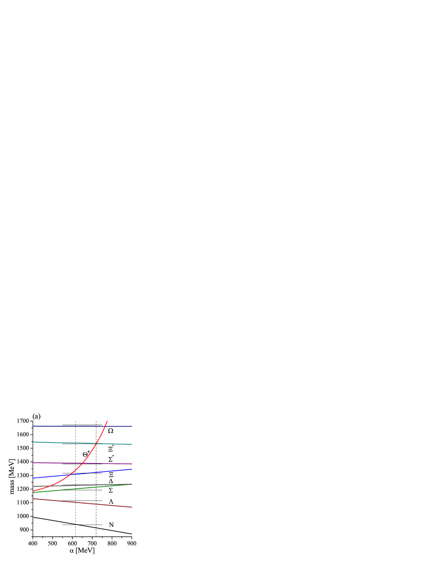
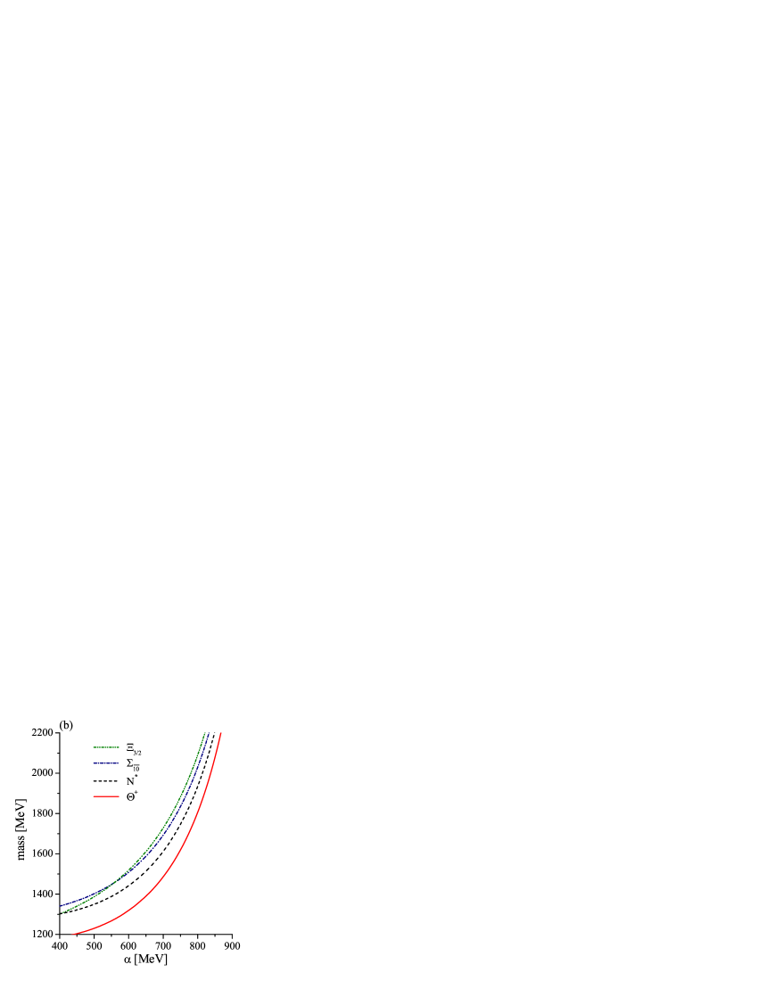
Figure 1: (a) Spectrum of the nonexotic baryons as a function of parameter $\alpha$, together with a prediction for the mass of $\Theta^{+}$. Thin horizontal lines correspond to the experimental data, dashed vertical lines correspond to fit II ($\alpha=615$) and fit I ($\alpha=720$).  (b) Spectrum of the exotic antidecuplet as a function of parameter $\alpha$.

Although there is rather large sensitivity of $M_{\Theta^{+}}$ to the choice of $\alpha$, the conclusion one can draw from Fig.1.a is that $\Theta^{+}$ is relatively light. The full spectrum of the exotic antidecuplet as a function of parameter $\alpha$ is shown in Fig.1.b We see that below $\alpha=600$ MeV the second order correction reshuffles the order of the antidecuplet states which means that the perturbation theory becomes unreliable. As compared to the first order perturbation theory, the states are no longer equally spaced, with $\Theta^{+}$ being significantly lighter than the other members of $\overline{10}$. It is interesting to note that if we fixed the value of $I_{2}$ (or equivalently $\alpha$) by the requirement that $M_{\text{N}^{\ast}}=1710$ MeV, we would get $\alpha=738$ MeV corresponding to $\Theta^{+}$ mass of $1580$ MeV.

Finally let us present another estimate of $I_{2}$ based on the model formulae for the parameters of Hamiltonian $H_{0}$ in the first order of the perturbation theory. These parameters depend on the soliton size, $r_{0}$, which enters the convenient variational Ansatz [32] of the soliton profile function $P(r)$ (2):

$$P(r)=2\arctan\left[\left(\frac{r_{0}}{r}\right)^{2}\right].$$ (25)

In practice one uses dimensionless variable $x_{0}=eF_{\pi}r_{0}$. Here $e$ is a free parameter corresponding to the Skyrme term in the mesonic Lagrangian (1) and $F_{\pi}=186$ MeV (for the details see e.g. Ref.[33]). In Ref.[33] we have calculated $M_{\text{cl}}$, and $I_{1,2}$ in terms of $x_{0}$ for the arctan Ansatz (25):

$$M_{\mathrm{cl}} =\frac{F_{\pi}}{e}{\pi}^{2}\frac{3\sqrt{2}}{16}(4x_{0}+\frac{15}{x_{0}}),$$ (26)

$$I_{1} =\frac{1}{e^{3}F_{\pi}}\pi^{2}\frac{\sqrt{2}}{12}\,(6x_{0}^{3}+25x_{0}),$$ (27)

$$I_{2} =\frac{1}{e^{3}F_{\pi}}\pi^{2}\frac{\sqrt{2}}{16}\,(4x_{0}^{3}+9x_{0}).$$ (28)

By minimizing $M_{\text{cl}}$ with respect to the soliton size we get we get $x_{0}=\sqrt{15/4}$. It is easy to convince oneself that by fitting the octet–decuplet mass difference:

$$M_{10}-M_{8}=\frac{3}{2I_{1}}=231\;\text{MeV}$$ (29)

we get $e=4.64$. With this value of $e$ we have $1/I_{2}\simeq 400$ MeV and $M_{\overline{10}}=1762\;$MeV. Assuming that splittings in $\overline{10}$ are identical with the splittings in the ordinary decuplet (which is true in the first order of the perturbation theory for the breaking Hamiltonian (12)) we get $M_{\Theta^{+}}\simeq 1460$ MeV.

5. Comparison with the Chiral Quark Model

The authors of Ref.[13] used the mass formula in the first order in $m_{s}$ with, however, nonleading terms in $N_{c}$ (see Eq.(10)). The reason was, as in our case, that the mass formula in the leading order in $N_{c}$ and in $m_{s}$ (8) was unable to reproduce the nonexotic mass spectra with good enough accuracy. Systematic expansion of the rotational effective Hamiltonian in inverse powers of $N_{c}$ [26] introduces $3$ unknown free constants $\alpha^{\prime}$, $\beta$ and $\gamma$ to $H^{\prime}$ of Eq.(10). However, only two linear combinations enter the nonexotic mass splittings. Therefore the ordinary baryons allow to fix only $4$ parameters $M_{8}$, $M_{10}$ and the above mentioned two linear combinations of $\alpha^{\prime}$, $\beta$ and $\gamma$. In other words, in contrast to our approach, there is no way to fix $I_{2}$ without some further assumptions. Also the third linear combination of breaking parameters cannot be fixed. This is an important ingredient, because the exotic spectra are sensitive to other linear combinations of $\alpha^{\prime}$, $\beta$ and $\gamma$ [13].

The main uncertainty due to $I_{2}$ was removed in Ref.[13] by the assumption that the ”nucleonic” member of the antidecuplet was identified with the nucleon resonance N^∗(1710). The remaining freedom, illustrated in Fig.2.a was removed by fixing $m_{s}=150$ MeV and $\Sigma_{\pi N}=45$ MeV. How big is the residual uncertainty due to the choice of $m_{s}$ and $\Sigma_{\pi N}$? We illustrate this in Fig.2.b where we plot the spectrum of the antidecuplet states, for fixed N^∗(1710), as a function of a dimensionless parameter

$$S=\frac{m_{s}}{150}\frac{\Sigma_{\pi N}}{50}.$$ (30)

The choice of Ref.[13] corresponds to $S=0.9$. However, other choices of $S$ are phenomenologically not excluded. For example in Refs.[34] we have used parameterization with $\gamma=0$, as the explicit model calculations suggest [26], which corresponds to $S=1.16$. With this choice of $S$ we get $M_{\Theta^{+}}=1560$ MeV. This is very close to $1580$ MeV obtained within the Skyrme model second order perturbation theory by fixing N^∗ at $1710$ MeV.

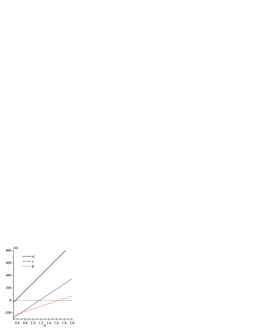
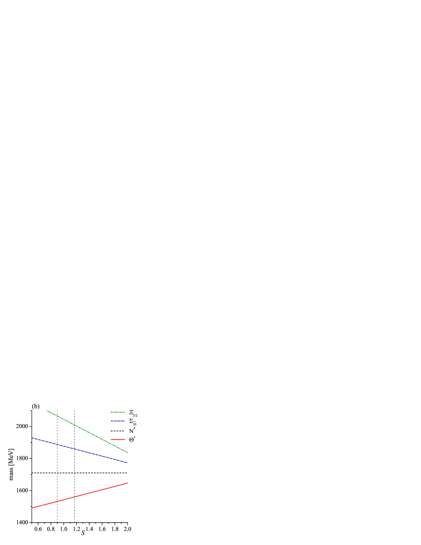
Figure 2: (a) Parameters  $\alpha^{\prime},\beta$ and  $\gamma$ as functions of  $S$ constrained to fit the nonexotic baryon spectra.  (b) Spectrum of antidecuplet in the Chiral Quark Model as a function of $S$. $S=0.9$ corresponds to the choice of Ref.[13], whereas $S=1.16$ corresponds to $\gamma=0$.

Our original choice of $m_{s}$ and $\Sigma_{\pi N}$ [12] corresponds to $S=1.6$, i.e. as seen from Fig.2.a, to $\beta=0$. Although in our approach $\gamma=0$ as well, however, the second order perturbation theory generates effects similar to $\gamma\neq 0$. Figure 2.a indicates that the good fit to the nonexotic spectra with $S=1.6$ requires rather large $\alpha\simeq 700$ MeV in agreement with our fit I.

6. Discussion and conclusions

The above discussion shows that chiral models predict the existence of the low lying exotic baryons. The precise value of the lightest member of the exotic antidecuplet depends crucially on the estimate of the strange moment of inertia $I_{2}$. We have presented two kinds of estimates of $I_{2}$. The one based on the second order mass formula for baryons, allowed us to fix $I_{2}$ from the spectrum of the nonexotic states . We used the second order perturbation theory in order to fit the nonexotic spectra with high accuracy. With our original choice of parameters for the pion-nucleon sigma term $\Sigma_{\pi N}=60$ MeV and the strange quark mass $m_{s}=200$ MeV we have predicted $M_{\Theta^{+}}=1534$ MeV. This number is in striking agreement with the latest experimental evidence, however, one should not forget that in fact the prediction of $M_{\Theta^{+}}$ depends rather strongly on the model parameters. If we used, as in Ref.[13], the mass of N${}^{\ast}(1710)$ to anchor the center of $\overline{10}$, we would get $M_{\Theta^{+}}=1560$. A similar analysis has been recently done in Ref.[35].

The second estimate of $I_{2}$ was based on the first order mass formula and on model expression for $I_{2}$ (28). With this method the mass of $\Theta^{+}$ comes out slightly lower; $M_{\Theta^{+}}\simeq 1460$.

The existence of the light, exotic, positive parity baryons belonging to antidecuplet is a natural feature of the chiral models [6],[10][11],[12]. From the beginning it was clear that the minimal quark content of such a multiplet must be $q^{4}\overline{q}$ [11]. Quark models, however, have difficulties in accommodating $\Theta^{+}$ of positive parity (yet requiring experimental confirmation) unless strong interquark correlations are introduced [36],[37]. Perhaps the most striking difference between the quark and the soliton pictures consists in the fact that in the quark models $\overline{10}$ is inevitably accompanied by an exotic octet which does not appear in the soliton approach. With the discovery of $\Theta^{+}$ low energy QCD regained attention and the constituent quark vs. soliton interpretations of the light baryons compete in explaining the data.

We would like to thank B. Jaffe, M. Polyakov, V. Petrov and K. Goeke for conversations. We benefited from the e-mail exchanges with K. Hicks, D.I. Diakonov, M. Karliner and H.J. Lipkin. This work was partly supported by the Polish State Committee for Scientific Research under grant 2 P03B 043 24.

References

- [1] LEPS Collaboration (T. Nakano et al.), Phys. Rev. Lett. 91 (2003) 012002.
- [2] DIANA Collaboration (V.V. Barmin et al.), hep-ex/0304040.
- [3] CLAS Collaboration (S. Stepanyan et al.), hep-ex/0307018.
- [4] SAPHIR Collaboration (J. Barth et al.), hep-ex/0307083.
- [5] A. Manohar, Nucl. Phys B248 (1984) 19.
- [6] M. Chemtob, Nucl. Phys. B256 (1985) 600.
- [7] E. Guadagnini, Nucl. Phys. B236 (1984) 35.
- [8] P.O. Mazur, M. Nowak and M. Praszałowicz, Phys. Lett. B147 (1984) 137.
- [9] S. Jain and S.R. Wadia, Nucl. Phys. B258 (1985) 713.
- [10] M.P. Mattis and M. Karliner, Phys. Rev. D34 (1986) 1991.
- [11] M. Karliner talk at Workshop on Skyrmions and Anomalies, M. Jeżabek and M. Praszałowicz editors, World Scientific 1987, page 164.
- [12] M. Praszałowicz, talk at Workshop on Skyrmions and Anomalies, M. Jeżabek and M. Praszałowicz editors, World Scientific 1987, page 112.
- [13] D.I. Diakonov, V.Yu. Petrov and M.V. Polyakov, Z. Phys. A359 (1997) 305.
- [14] For a review see D.I. Diakonov and V.Yu. Petrov, contribution to the Festschrift in honor of B.L. Ioffe, M. Shifman editor, At the frontier of particle physics, vol. 1, page 359, hep-ph/0009006; D.I. Diakonov, lectures given at Advanced Summer School on Nonperturbative Quantum Field Physics, Peniscola, Spain, 2-6 June 1997, Advanced school on non-perturbative quantum field physics 1-55, hep-ph/9802298.
- [15] Y. Nambu and G. Jona-Lasinio, Phys. Rev. 124 (1961) 246.
- [16] D.I. Dyakonov and V.Yu. Petrov, Nucl. Phys. B245 (1984) 259; B272 (1986) 457; E.V. Shuryak, Phys. Rep. 115 (1985) 15.
- [17] D.I. Dyakonov and M. Eides JETP Lett. 38 (1983) 433; J. Żuk, Z. Phys. 29 (1985) 303; M. Praszałowicz and G. Valencia, Nucl. Phys. B341 (1990) 27; E. Ruiz Arriola Phys. Lett. B253 (1991) 430.
- [18] T.H.R Skyrme, Proc. Royal Soc. A260 (1961) 127; Nucl. Phys. 31 (1962) 556.
- [19] J. Wess and B. Zumino, Phys. Lett. B37 (1971) 95.
- [20] E. Witten, Nucl. Phys. B160 (1979) 57; B223 (1983) 422; B223 (1983) 433.
- [21] G.S. Adkins, C.R. Nappi and E. Witten, Nucl. Phys. B228 (1983) 552; G.S. Adkins and C.R. Nappi, Nucl.Phys. B233 (1984) 109.
- [22] M. Praszałowicz, Phys. Lett. B158 (1985) 264.
- [23] For an extensive review of the SU(3) Skyrme Model see H. Weigel, Int. Jour. of. Mod. Phys., 11 (1996) 2419.
- [24] G.S. Adkins and C.R. Nappi, Nucl. Phys. B249 (1985) 507.
- [25] B. Moussallam and D. Kalafatis, Phys. Lett. B272 (1991) 196; B. Moussallam, Annals Phys. 225 (1993) 264.
- [26] A. Blotz, D.I. Diakonov, K. Goeke, N.W. Park, V.Yu. Petrov, P.V. Pobylitsa, Phys. Lett. B287 (1992) 29; Nucl. Phys. A555 (1993) 765; H. Weigel, R. Alkofer and H. Reinhardt, Phys. Lett. B284 (1992) 296.
- [27] J.J. De Swart, J. of Mod. Phys. 35 (1963) 916.
- [28] H. Yabu and K. Ando, Nucl. Phys. B301 (1988) 601.
- [29] M. Praszalowicz, Phys. Rev. D42 (1990) 216; P. Sieber, M. Praszalowicz and K. Goeke, Nucl. Phys. A569 (1994) 629.
- [30] R. Koch, Z. Phys. C15 (1982) 161; W. Wiedner et al., Phys. Rev. Lett. 58 (1987) 648; J. Gasser, H. Leutwyler, M.P. Locher and M.E. Sainio, Phys. Lett. B213 (1988) 85.
- [31] J. Gasser, H. Leutwyler and M.E. Sainio, Phys. Lett. B253 (1991) 252.
- [32] D.I. Dyakonov and V.Yu. Petrov, JETP Lett. 43 (1986) 57.
- [33] M. Praszałowicz, Acta Phys. Pol. B22 (1991) 525.
- [34] H-Ch. Kim, M. Praszałowicz and Klaus Goeke, Phys. Rev. D57 (1998) 2859, H-Ch. Kim, M. Praszałowicz, M.V. Polyakov and Klaus Goeke, Phys. Rev. D58 (1998) 114027.
- [35] V.B. Kopeliovich and H. Walliser, hep-ph/0304058.
- [36] R.L. Jaffe and F. Wilczek, hep-ph/0307341.
- [37] M. Karliner and H.J. Lipkin, hep-ph/0307243.