The self-consistent bounce: an improved nucleation rate

Abstract

We generalize the standard computation of homogeneous nucleation theory at zero temperature to a scenario in which the bubble shape is determined self-consistently with its quantum fluctuations. Studying two scalar models in 1+1 dimensions, we find the self-consistent bounce by employing a two-particle irreducible (2PI) effective action in imaginary time at the level of the Hartree approximation. We thus obtain an effective single bounce action which determines the rate exponent. We use collective coordinates to account for the translational invariance and the growth instability of the bubble and finally present a new nucleation rate prefactor. We compare the results with those obtained using the standard 1-loop approximation and show that the self-consistent rate can differ by several orders of magnitude.

I Introduction

During first order phase transitions, the macroscopic state of a system changes suddenly from the metastable phase (or false vacuum) to the stable phase (or true vacuum). If the transition is strongly first order it is expected to proceed by the spontaneous creation of spherically symmetric droplets – or bubbles – of the stable phase which, if large enough, can grow to consume the metastable phase.

The modern theory of bubble nucleation is due principally to Langer Langer , who was concerned with models of statistical physics and to Voloshin Voloshin and Coleman and Callan Coleman ; CallanColeman who developed similar ideas in the context of relativistic (zero temperature) quantum field theory. The unification of Langer and Coleman’s approach to finite temperature quantum field theory was later obtained by Affleck Affleck and Linde Linde , among others.

Although the departure point for the theory of nucleation is completely general, in practice the nucleation rate is computed almost without exception in the semiclassical approximation, including fluctuations only at most to 1-loop order. Even for semirealistic models, these lowest order calculations can be computationally nontrivial Baacke . We quote the now well-known zero temperature result of Ref. CallanColeman that for $D$ spacetime dimensions, the nucleation rate per unit volume $\Gamma/V$ is given by

$$\Gamma/V=Ae^{-B},\quad B=S_{cl}[\phi_{b}]/\mathchar 1406\relax,\quad A=\left(\frac{B}{2\pi}\right)^{D/2}~{}\left|\frac{det^{\prime}\left[-\partial+V^{\prime\prime}(\phi_{b})\right]}{det\left[-\partial+V^{\prime\prime}(\phi_{+})\right]}\right|^{{-1/2}}$$ (1)

where $S_{cl}=\int d^{D}x(\partial_{x}\phi)^{2}/2+V(\phi)$ is the classical Euclidean action of the “bounce” and $det^{\prime}$ denotes, as usual, the fluctuation determinant with $D$ zero modes excluded.

Nevertheless in certain instances, an improvement on the 1-loop computation is necessary, for example when the first order character of the transition is itself due to radiative corrections or to the presence of other fields, as in Higgs + gauge theories. It would seem that, at least to lowest order again, these effects might be accounted for by substituting an effective potential for the classical one in the bounce computation or more generally employing an effective action Weinberg ; Strumia . But this is not a simple task as fluctuations exist over the bubble background, and this background may distort significantly the properties of the low lying spectrum relative to its perturbative form.

One resolution to this problem is a different treatment of low and high energy fluctuations, for example in the context of a coarse-grained effective action Strumia ; Wetterich ; O'ConnorStephens . In such a procedure, however, much care must be taken to avoid double counting the effects of fluctuations, i.e. in their accounting for distortion of the bubble while also providing corrections to the background in which the bubble exists. Certain physical effects such as fluctuation backreaction on the classical bubble profile are usually absent from these calculations. Finally, lattice Monte Carlo methods have also been used to study nucleation rates, including more recently for the case of radiatively induced transitions Alford ; Moore .

In this paper we propose a self-consistently improved nucleation rate by including all of the above features in a semi-analytical computation Surig . We shall study two scalar models in 1+1 dimensions and include the self-coupling of fluctuations as well as their backreaction on the mean field nonperturbatively through the use of a two-particle irreducible (2PI) effective action formalism. We have also used this technique recently to calculate the self-consistent quantum energies of topological defects kinkpaper .

The organization of the paper is as follows: in Sec. II we review aspects of the constuction of the rate as defined in Eq. (1) as some of these will need to be modified later. We define our scalar models in Sec. III and give a short overview of the 2PI effective action formalism we employ. We also define the quantum bounce in terms of coupled Euclidean spacetime equations for the mean field and the coincident two-point function. In Sec. IV we discuss the renormalization structure of counterterms necessary to make these calculations finite. We present numerical results for the quantum bounce profiles and corresponding effective action calculations in Sec. V and also discuss the spectrum of fluctuations in the self-consistent case vs at 1-loop order. Finally in Sec. VI we discuss how to extract the nucleation probability in the self-consistent case and propose a new nucleation rate. A brief discussion of the results is offered in Sec. VII

II Structure of the rate calculation

The 1-loop approximation to the rate calculation leading to Eq. (1) has several special features, which we now highlight in order to be able to contrast them with our results below. We will take $\mathchar 1406\relax=1$ throughout and work in $D$-dimensional Euclidean spacetime, although later we shall specialize to $D=2$.

The starting point of any rate calculation is the transition amplitude

$$\langle\phi_{+}(x)|\phi_{-}(x^{\prime})\rangle={\cal N}\int d[\phi]e^{-S[\phi]/\mathchar 1406\relax}={\cal Z},$$ (2)

with appropriate boundary conditions on the fields. We are interested in a transition amplitude between the false and true vacua, i.e. the vacuum expectation value of the field is given by the true vacuum at some spacetime point, taken to be the origin $\langle\phi(x^{\mu}=0)\rangle=\phi_{-}$, and in the false vacuum at spacetime infinity $\langle\phi(x^{\mu}\rightarrow\infty)\rangle=\phi_{+}$. The normalization $\cal N$ ensures that

$$\langle\phi_{+}(x)|\phi_{+}(x^{\prime})\rangle=\langle\phi_{-}(x)|\phi_{-}(x^{\prime})\rangle=1.$$ (3)

In the semiclassical approximation the path integral is evaluated by expanding around the field configurations that extremize the classical action, subject to these boundary conditions. The simplest such configuration is the classical bounce $\phi_{b}$. Well separated multi-bounce configurations also qualify and need to be summed over among the action extrema.

The single bounce path integral can be evaluated semiclassically (i.e. to 1-loop order) by expanding the quantum field in linearized fluctuations around the classical bounce configuration

$$\phi=\phi_{b}+\sum_{n}a_{n}\psi_{n}.$$ (4)

Then the (renormalized) path integral becomes

$${\cal Z}={\cal N}Ae^{-B};\qquad A=\left|\frac{det\left[-\partial+V^{\prime\prime}(\phi_{b})\right]}{det\left[-\partial+V^{\prime\prime}(\phi_{+})\right]}\right|^{-1/2};\quad B=S_{cl}[\phi_{b}]$$ (5)

where we took the fluctuations to be eigenstates of the linearized operator $G^{-1}_{0}=-\partial+V^{\prime\prime}(\phi)$. Defined as such, the fluctuations are non self-interacting and do not backreact on the profile $\phi_{b}$ (i.e. neither the operator $G_{0}$ nor the equation of motion solved by $\phi_{b}$ depends on the fluctuations $\psi_{n}$).

Note that $\cal Z$ is dimensionless as it should be for a probability. There is a simple functional relation between $\cal Z$ and the effective action $\Gamma_{\rm eff}$. In the absence of external sources

$${\cal Z}=e^{-\Gamma_{\rm eff}}$$ (6)

and the 1-loop effective action takes the well known form $\Gamma_{\rm eff}=B-\frac{1}{2}\ln A$.

Given the transition amplitude due to one bounce, it is straightforward to generalize to any number of bounces. This is the sum of the 1-bounce contribution plus the 2-bounce contribution, which for well separated configurations becomes the product of two single bounces, etc. The result of resumming this series is the exponentiation of the single bounce amplitude i.e.

$$Z=\exp[e^{-B}A]=\exp[e^{-\Gamma_{\rm eff}}]$$ (7)

The nucleation rate (per unit volume) has dimensions of inverse spacetime volume and can be obtained directly from the multi-bounce amplitude as

$$\Gamma/V=2\ \hbox{Im}\left({1\over\Omega}\ln{\cal Z}\right),$$ (8)

where $\Omega$ is the spacetime volume. (We regret the confusing notation which arises since the capital letter $\Gamma$ serves as the conventional standard for both the rate and the effective action. We use $\Gamma_{\rm eff}$ where necessary to avoid ambiguity.)

To see that this result is finite in the infinite volume limit, we must analyze the determinant ratio in the prefactor $A$ in greater detail. To 1-loop order, it is well known that the fluctuation spectrum has one negative eigenvalue (an imaginary frequency) and $D$ zero eigenvalues. The former keeps track of the instability of the false vacuum. In a theory without backreaction this instability is connected with a nonconservation of a probability current CallanColeman ; Affleck , a mode that will grow unchecked in the large spacetime volume. The $D$ zero modes are proportional to the $D$ variations $\partial_{\vec{x}}\phi_{b}$, and represent the translational invariance of the “center” of the classical bounce.

Each eigenvalue in the determinant $A$ results from a Gaussian integration

$$\frac{1}{\omega}=\frac{1}{2\pi}\int d\psi e^{-\psi{\omega^{2}_{i}\over 2}\psi}.$$ (9)

This integral is clearly divergent if $\omega^{2}$ is negative, but it is rendered sensible by deformation of the contour into the complex plane (in effect taking $\omega^{2}\rightarrow|\omega^{2}|$). Thus the amplitude $\cal Z$ is imaginary, reflecting the fluctuation instability. (As the nucleation–or decay–rate is determined by the imaginary part of the transition amplitude, one simply excises the factor of $i$).

In the case $\omega\rightarrow 0$ the corresponding integral is of course not Gaussian at all. It becomes, up to a Jacobian factor, the volume and diverges with it. This is clear from the change of variables

$$[d\phi]i=Jdz,\qquad J=\left[\int d^{D}x\left(\frac{\partial\phi(x,z)}{\partial x}\right)^{2}\right]^{1/2},$$ (10)

$$\lim_{\omega\rightarrow 0}\frac{1}{\omega}=\sqrt{\frac{1}{2\pi}}J\int dz=\frac{J}{\sqrt{2\pi}}\Omega^{1/D},$$ (11)

with the linear volume $\Omega^{1/D}\rightarrow\infty$. What we have done is exchange the functional integration over the field direction $[d\phi]$ for an integration over a collective coordinate $z$. The zero modes thus give rise to an infrared divergence (related to the limit of infinite spacetime volume) in the determinant prefactor. This factor of volume is happily canceled as the probability amplitude, taken per unit spacetime volume, becomes the desired rate per volume of Eq. (1). Namely

$$\frac{1}{\Omega}\left|\frac{det\left[-\partial+U^{\prime\prime}(\phi_{b})\right]}{det\left[-\partial+U^{\prime\prime}(\phi_{+})\right]}\right|^{-1/2}\rightarrow\left(\frac{J}{\sqrt{2\pi}}\right)^{D}\left|\frac{det^{\prime}\left[-\partial+U^{\prime\prime}(\phi_{b})\right]}{det\left[-\partial+U^{\prime\prime}(\phi_{+})\right]}\right|^{-1/2}.$$ (12)

(In a finite volume application, it is quite reasonable that the nucleation rate grows as a function of volume.)

There are two distinct ways in which this standard calculation is approximate. The first is the computation of the single-bounce effective action. The semi-classical or 1-loop approximation is a lowest order calculation of the effects of fluctuations. It completely neglects both fluctuation self-interactions and their backreaction on the classical field profile. Because barrier nucleation is a Boltzmann-suppressed process, exponentially sensitive to corrections, the inclusion of these effects may lead to large quantitative differences. A computation of the nucleation rate that includes these effects is the subject of the present paper.

The second approximation involved in the rate calculation is the “dilute instanton approximation” CallanColeman ; tHooft for the multi-bounce configurations. This is in principle justified so long as the nucleation rate per volume is sufficiently small. It will not be a good approximation though in cases where nucleation may be enhanced by earlier bubbles or by the presence of other nonperturbative fluctuations over the homogeneous background. Although some of these situations could be addressed with the techniques developed here we will not explore them in the present manuscript. We will thus continue to assume the dilute instanton approximation as an unaltered ingredient of the rate computation.

III 2PI Effective Action

The traditional starting point for the calculation of the single bounce is the classical action. We refer the reader to the Ref. Coleman for that formalism and do not summarize it extensively here. Suffice it to say that the classical bounce is an $O(D)$-symmetric solution to the Euclidean field equations in $D$ spacetime dimensions satisfying certain boundary conditions, in particular that the field assumes a true vacuum expectation value in a local region around the origin and a false vacuum expectation value far away and to infinity. In our development of the self-consistent bounce, we begin instead with the two-particle irreducible (2PI) effective action for the field $\phi$ and the two-point function $G(x,x^{\prime})$ developed in the relativistic context by Cornwall, Jackiw and Tomboulis (CJT) 2PI .

The effective action functional is given by

$$\Gamma(\phi,G)=I(\phi)+\frac{1}{2}i\hbox{Tr}\ln D_{0}G^{-1}+\frac{1}{2}i\hbox{Tr}D^{-1}(\phi)G+\Gamma_{2}(\phi,G)+\hbox{const}$$ (13)

In this notation we have the classical action

$$I(\phi)=\int d^{2}x{\cal L}[\phi],\qquad{\cal L}[\phi]=\frac{1}{2}\partial_{\mu}\phi\partial^{\mu}\phi-V(\phi)$$ (14)

and the operator

$$iD^{-1}(x,x^{\prime};\phi) = \frac{\delta^{2}I}{\delta\phi(x)\delta\phi(x^{\prime})}.$$ (15)

$D_{0}$ is the free propagator. Finally $\Gamma_{2}$ sums the 2PI vacuum to vacuum diagrams which furnish an expansion in the number of loops or, equivalently, in powers of $\mathchar 1406\relax$ ($\mathchar 1406\relax=c=1$ below and throughout). Stationarizing the action leads to the equations:

$$\frac{\delta I}{\delta\phi}+\frac{1}{2}iG\frac{\delta D^{-1}}{\delta\phi}+\frac{\delta\Gamma_{2}}{\delta\phi} = 0$$ (16)

$$-\frac{1}{2}iG^{-1}+\frac{1}{2}iD^{-1}+\frac{\delta\Gamma_{2}}{\delta G} = 0$$ (17)

We shall consider two symmetry-breaking forms for the scalar potential

$$V_{4}(\phi) = \frac{1}{4}\lambda\left[(\phi^{2}-v^{2})^{2}-\frac{2\epsilon}{\lambda v}(\phi+v)\right]\qquad v^{2}=\frac{\mu^{2}}{\lambda}$$ (18)

$$V_{6}(\phi) = \frac{1}{2}\lambda\phi^{2}\left[(\phi^{2}-a^{2})^{2}-\frac{2\epsilon}{\lambda a^{2}}\right]\qquad a^{2}=\frac{\mu}{\sqrt{\lambda}}$$ (19)

These potentials represent more or less generic models with true and false vacua at the classical level and have been cast in the form that the potential difference between the true and false vacua is $\epsilon$. The symmetry is explicitly broken in the quartic model while a $\phi\rightarrow-\phi$ discrete symmetry still exists in the sextic model (where the false vacuum is the symmetric minimum $\phi=0$). The quantization of solitons in (1+1)-dimensional models of precisely these types with $\epsilon=0$ were originally examined in Ref. Lohe .

For these models we obtain the following equations: for $V_{4}$,

$$\Box\phi+\frac{1}{2}\lambda\left[2\phi(\phi^{2}-v^{2})-\frac{\epsilon}{\lambda v}\right]+3\lambda\phi G(x,x)-\frac{\delta\Gamma_{2}}{\delta\phi}=0$$ (20)

$$iG^{-1}(x,x^{\prime})+\left(\Box_{x}-\lambda v^{2}+3\lambda\phi^{2}\right)\delta^{2}(x-x^{\prime})-2\frac{\delta\Gamma_{2}}{\delta G}=0$$ (21)

and for $V_{6}$,

$$\Box\phi+\lambda\phi\left[(\phi^{2}-a^{2})^{2}+2\phi^{2}(\phi^{2}-a^{2})-\frac{2\epsilon}{\lambda a^{2}}\right]-6\lambda\left(2a^{2}\phi-5\phi^{3}\right)G(x,x)-\frac{\delta\Gamma_{2}}{\delta\phi}=0$$

(22)

$$iG^{-1}(x,x^{\prime})+\left[\Box_{x}+\lambda(a^{4}-\frac{2\epsilon}{\lambda a^{2}})-12\lambda a^{2}\phi^{2}+15\lambda\phi^{4}\right]\delta^{2}(x-x^{\prime})-2\frac{\delta\Gamma_{2}}{\delta G}=0$$

(23)

Up to this point we have made no approximations, but we have left $\Gamma_{2}$ as the sum of 2PI vacuum-to-vacuum diagrams with interaction vertices determined by the shifted Lagrangian and lines representing the full propagator $G$. For our models, we can summarize the interactions in Table 1.

vertex		$I_{4}$		$I_{6}$
cubic		$-\lambda\phi$		$-2\lambda(5\phi^{3}-2a^{2}\phi)$
quartic		$-\frac{\lambda}{4}$		$-\frac{\lambda}{2}(15\phi^{2}-2a^{2})$
quintic				$-3\lambda\phi$
sextic				$-\frac{\lambda}{2}$

Table 1: Interaction vertices used in the construction of the 2PI effective action for two models

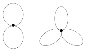
Figure 1: Vacuum bubble diagrams in the Hartree approximation for the 2PI effective action of our models. For the classical action $V_{4}$, only the left diagram contributes. Lines denote the full propagator $G$ in the nontrivial $\phi$ background.

It is of practical necessity in the computation to select only certain 2PI diagrams, and such a choice will correspond to a truncation in the Dyson-Schwinger hierarchy of equations for the correlation functions of the model. It is straightforward to write down the full evolution equations in the Hartree approximation, which amounts to including only the 2PI “bubble” diagrams shown in Fig. 1. In $O(N)$ models, this truncation is similar to the leading-order large-$N$ approximation. While the Hartree approximation is not a controlled, systematic expansion, it is understood to be equivalent to a Gaussian variational ansatz in the Schrödinger functional formalism Schroedinger and results in Hamiltonian dynamics Hamiltonian . Furthermore, a study of the quantum energy of solitons showed good agreement between the Hartree values and “exact” lattice Monte Carlo results kinkpaper ; salle . Proceeding with the approximation, we find

$$\Gamma_{2}^{V_{4}} = -\frac{3}{4}\lambda\int d^{2}xG(x,x)^{2}$$ (24)

$$\Gamma_{2}^{V_{6}} = -\frac{3}{2}\lambda\int d^{2}x(15\phi(x)^{2}-2a^{2})G(x,x)^{2}-\frac{15}{2}\lambda\int d^{2}xG(x,x)^{3}\ .$$ (25)

so we obtain for $V_{4}$ (after inverting the $G$ equation),

$$\Box\phi+\frac{1}{2}\lambda\left[2\phi(\phi^{2}-v^{2})-\frac{\epsilon}{\lambda v}\right]+3\lambda\phi G(x,x)=0$$ (26)

$$\left[\Box_{x}-\lambda v^{2}+3\lambda\phi^{2}+3\lambda G(x,x)\right]G(x,x^{\prime})=-i\delta^{2}(x-x^{\prime})$$ (27)

and for $V_{6}$,

$$\left[\Box+\lambda\left[(\phi^{2}-a^{2})^{2}+2\phi^{2}(\phi^{2}-a^{2})-\frac{2\epsilon}{v}\right]\right.$$

$$\qquad-\left.6\lambda\left(2a^{2}-5\phi^{2}\right)G(x,x)+45\lambda G(x,x)^{2}\right]\phi=0$$

$$\left[\Box_{x}+\lambda(a^{4}-\frac{2\epsilon}{\lambda a^{2}})-12\lambda a^{2}\phi^{2}+15\lambda\phi^{4}\right.$$

$$\qquad\left.+6\lambda(15\phi^{2}-2a^{2})G(x,x)+45\lambda G(x,x)^{2}\right]G(x,x^{\prime})=-i\delta^{2}(x-x^{\prime})$$

(29)

This formal procedure has absorbed the approximate quantum dynamics of the scalar field $\phi$ into a truncated set of equations to be solved simultaneously. The two-point function $G(x,x^{\prime})$ now appears explicitly as a “sort of” Green’s function, albeit of a nonlinear operator which depends on its value at coincident spacetime points. Typically we would proceed by decomposing $G(x,x^{\prime})$ in a mode basis (related to the decomposition of the field operator of which it is a correlation function). The mode functions and the field then satisfy a tower of partial differential equations which can be stepped forward in time on a computer. This would be a prescription for the nonequilibrium evolution given Cauchy-type initial conditions stepbeyond .

III.1 Imaginary Time

We shall alternately consider attempting to solve Eqs. (26)-(29) in imaginary time. Passing to Euclidean spacetime and framing the partial differential equations as elliptical equations instead of hyperbolic ones does not in and of itself simplify the problem unless we can exploit special symmetries. This is precisely what is done in the case of the bounce, where as a consequence of Lorentz invariance we seek a rotationally invariant classical solution, i.e. we need solve only for radial functions. We can now see why at least at the level of the Hartree approximation, we can attempt a similar sleight of hand on the two-point function and the field simultaneously. Wherever the two-point function appears in the evolution operators, it appears with coincident spacetime arguments. Therefore, we can seek solutions to Eqs. (26)-(29) in imaginary time in which both $\phi(x)$ and $G(x,x)$ depend only on the radial coordinate in Euclidean spacetime.

To wit, the imaginary time formulation of the problem entails,

$$t\rightarrow i\tau,\qquad\Box\rightarrow\Box_{E}=-\nabla^{2}$$ (30)

or going to polar coordinates

$$\Box_{E}=-\frac{1}{\rho}\frac{\partial}{\partial\rho}\left(\rho\frac{\partial}{\partial\rho}\right)-\frac{1}{\rho^{2}}\frac{\partial^{2}}{\partial\theta^{2}}$$ (31)

We seek a solution to the field VEV and two-point function equations where the field VEV and the coincident two-point function are purely radial, i.e.

$$\phi=\phi(\rho),\qquad\qquad G(\rho,\theta;\rho,\theta)=G(\rho)$$

while in general there remains $\theta$-dependence in $G(\rho,\theta;\rho^{\prime},\theta^{\prime})$. It is consistent with these constraints to separate variables in which case $G$ takes the form

$$G(\rho,\theta;\rho^{\prime},\theta^{\prime})=\sum_{n,l}a_{nl}R_{nl}(\rho)R_{nl}(\rho^{\prime})e^{il(\theta-\theta^{\prime})}$$ (32)

The $\phi$ equations (26) and (III) become

$$\Box_{E}\phi+\frac{1}{2}\lambda\left[2\phi(\phi^{2}-v^{2})-\frac{\epsilon}{\lambda v}\right]+3\lambda\phi G(\rho)=0$$ (33)

$$\left[\Box_{E}+\lambda\left((\phi^{2}-a^{2})^{2}+2\phi^{2}(\phi^{2}-a^{2})-\frac{2\epsilon}{\lambda a^{2}}\right)\right.$$

$$\qquad-\left.6\lambda\left(2a^{2}-5\phi^{2}\right)G(\rho)+45\lambda G(\rho)^{2}\right]\phi(\rho)=0$$ (34)

and the equations

$$\left[\Box_{\rm E}+\chi(\rho)\right]G(\rho,\theta;\rho^{\prime},\theta^{\prime})=\frac{1}{\rho}\delta(\rho-\rho^{\prime})\delta(\theta-\theta^{\prime}),$$ (35)

$$\chi_{4}(\rho)=-m^{2}+3\lambda\phi^{2}+3\lambda G(\rho).$$

$$\chi_{6}(\rho)=\lambda(a^{4}-\frac{2\epsilon}{\lambda a^{2}})-12\lambda a^{2}\phi^{2}+15\lambda\phi^{4}+6\lambda(15\phi^{2}-2a^{2})G(\rho)+45\lambda G(\rho)^{2}.$$

lead to the following “nonlinear eigenvalue” problem for the radial modes

$$\left[-\frac{1}{\rho}\frac{\partial}{\partial\rho}\left(\rho\frac{\partial}{\partial\rho}\right)+\frac{l^{2}}{\rho^{2}}+\chi(\rho)\right]R_{nl}=\omega^{2}_{nl}R_{nl}.$$ (36)

with the identification

$$a_{nl}^{-1}=\omega^{2}_{nl},\qquad G(\rho)=\sum_{n,l}\frac{R^{2}_{nl}(\rho)}{\omega^{2}_{nl}}$$ (37)

provided the orthonormality and integrability condition holds for the $R_{nl}(\rho)$,

$$2\pi\int_{0}^{\infty}\rho d\rho R_{nl}(\rho)R_{mk}(\rho)=\delta_{nm,kl}$$ (38)

We must also impose boundary conditions at the origin $\rho=0$, where for analyticity we require that $G$ have zero derivative, and at large values of $\rho$ where $G$ should approach its value in the false vacuum. We impose the first condition on the radial mode functions $R_{nl}(\rho)$ whereby for $l=0$ the functions must have zero derivative at the origin and for $l\neq 0$ they must vanish. The condition at large $\rho$ can be made consistent with Dirichlet boundary conditions. This latter condition is especially suitable if the renormalized value of $G$ is fixed to be zero in the false vacuum. We shall discuss this renormalization condition in the following section.

IV Renormalization of Self-consistent Effective Action

Although any scalar model in 1+1 dimensions is super-renormalizable, details of the renormalization differ slightly in the self-consistent effective action from the usual loop expansion. Moreover numerical implementation of renormalization schemes comes with its own subtleties. Here we detail the procedure for a simplified $\phi^{4}$ model, i.e. with no symmetry breaking parameter $\epsilon$, in two steps. We first demonstrate the analytical cancellation of divergences assuming a homogeneous background. This may be considered a review of the renormalization of the self-consistent effective potential as worked out previously, for example in Ref. ACP . Next we describe the changes which occur for the inhomogeneous case of interest and for a finite volume with a discrete spectrum–as is the case in any numerical analysis.

For homogeneous fields we consider the effective potential and pass to Euclidean momentum space for the translationally invariant two-point function, i.e.

$$V(\phi,G)\int d^{2}x=\Gamma(\phi,G),$$ (39)

$$G(x,x^{\prime})=\int\frac{d^{2}k}{(2\pi)^{2}}e^{-ik(x-x^{\prime})}G(k)\equiv\int_{k}e^{-ik(x-x^{\prime})}G(k),$$ (40)

such that

$$V(\phi,G) = V_{cl}(\phi)+\frac{1}{2}\int_{k}\,\ln D_{0}G^{-1}+\frac{1}{2}\int_{k}\,\left[D^{-1}G-1\right]+\frac{3\lambda}{4}\Bigl{[}\int_{k}\,G(k)\Bigr{]}^{2}$$ (41)

Now setting $\frac{\delta V}{\delta G}=0$, we have

$$G^{-1}(k)=D^{-1}(k)+3\lambda\int_{k}\,G(k)$$ (42)

and taking as an ansatz $G(k)=\frac{1}{k^{2}+M^{2}}$, we obtain a gap equation for $M^{2}$:

$$M^{2}=-m^{2}+3\lambda\phi^{2}+3\lambda\int\frac{d^{2}k}{(2\pi)^{2}}\frac{1}{k^{2}+M(\phi)^{2}}$$ (43)

The integral in the gap equation is logarithmically divergent, hence $M^{2}$ is so far undefined. We now demonstrate the counterterm procedure which renormalizes this equation and also renormalizes the effective potential. We first rewrite the equation as

$$M^{2}=-m^{2}+3\lambda\phi^{2}+3\lambda\left(\int\frac{d^{2}k}{(2\pi)^{2}}\frac{1}{k^{2}+M(\phi)^{2}}-I\right)+3\lambda I$$ (44)

and impose a momentum cutoff $\Lambda$ with

$$I=\int^{\Lambda}\frac{d^{2}k}{(2\pi)^{2}}G_{0}(k)\equiv\int^{\Lambda}\frac{d^{2}k}{(2\pi)^{2}}\frac{1}{k^{2}+\mu_{0}^{2}}=\frac{1}{4\pi}\ln\frac{\Lambda^{2}}{\mu_{0}^{2}}.$$ (45)

This implements the regularization of the integrals in Eq. (44). The new scale $\mu_{0}$ is necessary to prevent an infrared logarithmic divergence in the infinite volume limit. The renormalization procedure is now carried out by identifying the bare parameter $m^{2}$ as a function of the cutoffs and defining a renormalized (physical) mass by

$$-m_{R}^{2}=-m^{2}+\delta m_{1}^{2}=-m^{2}+3\lambda I$$ (46)

In terms of the renormalized mass, the gap equation is finite

$$M^{2} = -m_{R}^{2}+3\lambda\phi^{2}+\frac{3\lambda}{4\pi}\ln\frac{\mu_{0}^{2}}{M^{2}}$$ (47)

$$= -m_{R}^{2}+3\lambda\phi^{2}+3\lambda G_{f}(M).$$ (48)

and we can see that by a choice of renormalization scale ($\mu_{0}^{2}=2m_{R}^{2}$), the self-consistent fluctuation mass in the classical vacuum $\phi_{0}^{2}=m_{R}^{2}/\lambda$ can be fixed to its “classical” value $M^{2}=2m_{R}^{2}$. We shall consider $\mu_{0}$ to be a physical scale, a function of the physical mass and couplings.

We now express the Hartree resummed effective potential in terms of its contributions at different orders, following Ref. ACP .

$$V_{eff}=V_{0}+V_{1}+V_{2}$$ (49)

Substituting Eq. (42) into (41), we now have

$$V_{0} = V_{cl}=-\frac{1}{2}m^{2}\phi^{2}+\frac{\lambda}{4}\phi^{4}$$

$$V_{1} = \frac{1}{2}\hbox{Tr}\ln D_{0}G^{-1}=\frac{1}{2}\int\frac{d^{2}k}{(2\pi)^{2}}\ln\left[\frac{k^{2}+M^{2}}{k^{2}+\mu_{0}^{2}}\right]$$

$$V_{2} = -\frac{3\lambda}{4}G(x,x)^{2}=-\frac{3\lambda}{4}\left(\int\frac{d^{2}k}{(2\pi)^{2}}\frac{1}{k^{2}+M^{2}}\right)^{2}\ ,$$ (50)

Note that as a simplification this classical potential has no symmetry breaking term and no overall constant. The constant has no physical significance, but we will in any case make the shift in the potential explicit below by subtracting the value at a specified vacuum. The symmetry breaking coupling introduces no new infinities and requires no renormalization.

We use (43) to write

$$G(x,x)=\frac{1}{3\lambda}\left(M^{2}-m^{2}-3\lambda\phi^{2}\right),$$ (51)

and

$$V_{0}+V_{2}=-\frac{M^{4}}{12\lambda}-\frac{1}{2}\lambda\phi^{4}+\frac{1}{6\lambda}M^{2}m^{2}+\frac{1}{2}M^{2}\phi^{2},$$ (52)

(where an additive constant has again been removed). We rewrite in terms of renormalized parameters,

$$-m^{2}=-m_{R}^{2}-3\lambda I,\qquad I=G_{0}(x,x)=\frac{1}{4\pi}\ln\frac{\Lambda^{2}}{\mu_{0}^{2}}$$ (53)

and use the renormalized gap equation (48) to write

$$\frac{1}{2}M^{2}G_{f}(M)=\frac{1}{6\lambda}M^{4}+\frac{M^{2}m_{R}^{2}}{6\lambda}-\frac{1}{2}M^{2}\phi^{2},$$ (54)

such that

$$(V_{0}+V_{2})^{R}=\frac{M^{4}}{12\lambda}-\frac{1}{2}\lambda\phi^{4}-\frac{1}{2}M^{2}G_{f}(M)-\frac{1}{2}M^{2}I.$$ (55)

Finally, the one-loop contribution to the potential comes to

$$V_{1} = \frac{1}{2}\int\frac{d^{2}k}{(2\pi)^{2}}\ln\left[\frac{k^{2}+M^{2}}{k^{2}+\mu_{0}^{2}}\right]$$ (56)

$$= \frac{1}{8\pi}(M^{2}-\mu_{0}^{2})\left(1+\ln\frac{\mu_{0}^{2}}{M^{2}}\right)+\frac{1}{2}(M^{2}-\mu_{0}^{2})I.$$ (57)

After shifting the combined tree-level and 2PI pieces of the effective potential by their contribution in the classical vacuum $\phi_{0}^{2}=m_{R}^{2}/\lambda$ (where the renormalization scale is set), the renormalized total is

$$V_{eff}=-\frac{1}{2}\lambda(\phi^{4}-\phi_{0}^{4})+\frac{M^{4}-\mu_{0}^{4}}{12\lambda}+\frac{1}{8\pi}(M^{2}-\mu_{0}^{2}),$$ (58)

which is finite.

The generalization of the effective potential to the effective Euclidean action for inhomogeneous mean field background now follows. We no longer have a simple gap equation, however the classical field $\chi$ defined in Eq. (35) now replaces the $M^{2}$ in the above analysis. The counterterm renormalization goes through and renders the tree level and 2PI components as a finite piece, expressed in terms of renormalized parameters, plus a counterterm:

$$\Gamma_{0+2}=\Gamma^{f}_{0+2}-\frac{1}{2}I\int dx\left(\chi(x)-\chi_{0}\right)$$ (59)

where

$$\Gamma^{f}_{0+2} = \int d^{2}x\left(\frac{1}{2}(\nabla\phi)^{2}+\frac{\chi^{2}(x)}{12\lambda}-\frac{1}{2}\lambda\phi^{4}-\frac{1}{2}\chi(x)G_{f}(x)-\frac{\chi_{0}^{2}}{12\lambda}+\frac{1}{2}\lambda\phi_{0}^{4}\right).$$ (60)

We have again chosen the mass scale of the counterterm to set $G_{f}(\phi_{0})=0$, so

$$\chi(x) = -m_{R}^{2}+3\lambda\phi^{2}(x)+3\lambda G_{f}(x),$$

$$\chi_{0} = -m_{R}^{2}+3\lambda\phi_{0}^{2},$$ (61)

and we could have equivalently written

$$\Gamma^{f}_{0+2} = \int d^{2}x\left(V_{cl}(\phi)-V_{cl}(\phi_{0})-\frac{3\lambda}{4}G_{f}(x,x)^{2}\right),$$ (62)

with $V_{cl}$ expressed in terms of renormalized (finite) parameters. Finally, the one-loop order contribution in the inhomogeneous case is obtained from the eigenvalues of Eq. (36).

$$\Gamma_{1} = \frac{1}{2}\sum\!\!\!\!\!\!\!\int\ln\frac{\omega^{2}_{nl}}{(\omega_{0}^{2})_{nl}},$$ (63)

by which we mean that $\omega^{2}_{nl}$ are the eigenvalues in the presence of the spatially varying field $\chi(\rho)$ and $(\omega_{0}^{2})_{nl}$ are the eigenvalues in the vacuum defined by $\chi_{0}$. This term is still logarithmically divergent, but this divergence is cancelled by the second term in Eq. (59) with

$$I\equiv G_{0}(\rho)=\sum_{n,l}\frac{(R_{0}^{2})_{nl}(\rho)}{(\omega_{0}^{2})_{nl}}.$$ (64)

The renormalization of the $\phi^{6}$ model follows along the same lines as above, although it is somewhat more cumbersome. In that case there occurs a renormalization of both the quadratic and quartic couplings. Both divergences have the same origin in the logarithmic loop integral of a gap equation analogous to Eq. (43), i.e. there is still only one renormalization scale.

There remains a subtlety in the practical computation of this one-loop term (63), which has been studied in the context of quantum corrections to static solitons kink . In that case, the quantity of interest is the sum over zero-point energies, or more precisely the difference of this sum in the presence of a soliton from this sum in the vacuum. Rebhan and van Nieuwenhuizen have pointed out that in the lattice discretized sum (for example in a finite volume) care must be taken in implementing a frequency cutoff for the sum such that the same number of modes are included in the vacuum sum and in the nontrivial sum (ambiguity arises because of both the presence of zero modes at the one-loop level and the phase shifts of the “continuum” states). We shall refer to this as a frequency cutoff with mode parity (FCMP) instead of a mode number cutoff as in Ref. kink . The analysis here of a spherically symmetric background in higher dimensions must follow the same prescription, and moreover the FCMP must be implemented separately for each angular quantum number. In other words, there is one frequency cutoff defined by the lattice spacing, but this leads to the inclusion of a different number of radial modes of each angular index included in the sum.

V The single bounce effective action

We have implemented the procedure described in the previous sections on a desktop workstation. Namely, we compute the vacuum counterterm (64) by solving the radial eigenvalue problem (36) in the false vacuum of each model. We then introduce a nontrivial mean field bubble of true vacuum (using the semi-classical bounce as an initial guess) and solve the renormalized versions of Eqs. (33)-(35) simultaneously by successive iteration. We use a standard relaxation routine Nrecipes to solve Eq. (33), together with a set of LAPACK packages LAPACK to solve the eigenvalue problem Eq.(36). At each step, the fluctuation eigenproblem is solved to produce a new intermediate $G_{\rm int}(x)$, which we combine with the old value to produce a new trial $G_{\rm new}=(1-\gamma)G_{\rm old}+\gamma G_{\rm int}$, until convergence in $\varphi$ and $G(x)$ is reached, up to a specified precision. The adjustable parameter $0<\gamma<1$ controls the size of the update and can be adapted to optimize convergence.

This numerical procedure will find the correct shape of the mean-field profile and the coincident two-point function if the radius is constrained. Unconstrained, however, it may fail to find the correct radius of the bubble, given the initial guess, since the stationary point of the action is a saddle point, not a minimum. (In other words, the successive iteration will not flow towards the saddle point.) The self-consistent bounce typically has a smaller radius than the classical bounce. We effectively constrain the radius first at its classical value and then vary the radius to find the actual saddle point.

The action is computed at each iterative step. It should be noted that the very first step of the procedure amounts to computing the fluctuation contribution to the action in the presence of the classical bounce without backreaction on the mean field or self-coupling of the fluctuation modes. In other words it is the standard 1-loop correction. Thus we are able to compare the value of the Euclidean action at the classical, 1-loop and self-consistent levels.

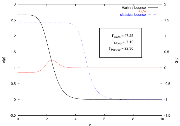
Figure 2: The self-consistent bounce and coincident two-point function for the $\phi^{6}$ model with parameters $\lambda/\mu^{2}=0.03,\epsilon/\mu^{2}=0.15$ are shown in solid lines. The dashed line is the (semi)classical bounce for this model. (Note that the $y$-axis for $G(\rho)$ is shifted with respect to the axis labeled by $\phi(\rho)$; $G$ still goes to zero in the false vacuum.) Inset: Euclidean action for various approximations.

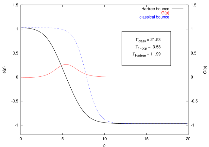
Figure 3: The self-consistent bounce and coincident two-point function for the $\phi^{4}$ model with parameters $\lambda/\mu^{2}=1,\epsilon/\mu^{2}=0.12$ are shown in solid lines. The dashed line is the (semi)classical bounce for this model. Inset: Euclidean action for various approximations.

In Figs. 2-3 we show the classical bounce along with the self-consistent bounce and the coincident two-point function for our two models. In the inset of each we give the value of the Euclidean action at the different orders of approximation. As the figures indicate, it is possible for the self-consistent bounce profile to differ significantly, both in radius and thickness, from the semi-classical prediction. Moreover the action, which will enter into our rate calculation, is dramatically different.

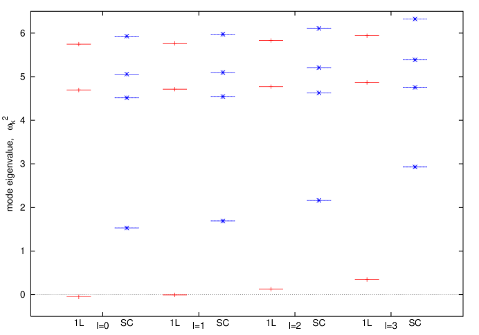
Figure 4: Spectra of the low lying fluctuation modes for the $\phi^{6}$ model. Plotted are the first few modes in the discrete spectrum for the first few partial waves, labeled by the quantum number $l$. The 1-loop spectra are shown side-by-side with the self-consistent spectra, with labels on the $x$-axis indicating 1L for 1-loop and SC for self-consistent.

It is important to mention also the difference between the self-consistent fluctuation spectrum and the 1-loop fluctuation spectrum. We display a plot of the low-lying spectra for the $\phi^{6}$ model in Fig. 4. Modes are labeled by radial and angular quantum numbers $n$ and $l$ in Eq.(36), and in the figure the $x$-axis proceeds along the increments in the angular number $l$. The 1-loop and self-consistent spectra for each $l$ are shown side-by-side for comparison. The numerical spectrum computed in a finite volume is of course discrete, but the lowest four states shown are actually bound states.

What is noteworthy is that the negative mode and the two zero modes of the 1-loop spectrum (each mode for $l\neq 0$ is doubly degenerate) are no longer negative or zero in the self-consistent spectrum. In fact, this is hardly surprising: once the fluctuation modes are allowed to interact in the presence of the bounce background, the spectrum will of course be shifted to positive values as the modes stabilize each other Boyanovsky ; kinkpaper . Needless to say this does not mean that translational invariance of the center of the bounce has been lost. Translational invariance is however no longer manifest at the level of linearized fluctuations since the mean field now cannot be translated without also translating the coincident two-point function $G$. We will return to the issues raised by this fact in the next section. For now it is perhaps most clearly illustrated at the level of the equations of motion.

Consider for example, the $\phi^{4}$ model. At the 1-loop level, we start with the usual equation of motion for the field and for linearized fluctuations around the bounce.

$$\Box\phi+V^{\prime}(\phi)=0$$ (65)

$$\left[\Box+V^{\prime\prime}(\phi)\right]\psi_{k}(x)=\omega^{2}_{k}\psi_{k}(x)$$ (66)

It is evident by taking the derivative of the field equation that each of the modes corresponding to translation of the field $\partial_{\vec{x}}\phi$ satisfy the fluctuation equation with zero eigenvalue. A similar trick will not work on the set of self-consistent equations in (26) and (27), which we recast below as follows:

$$\Box\phi+V^{\prime}(\phi)+3\lambda\phi G(x,x)=0$$ (67)

$$\left[\Box+V^{\prime\prime}(\phi)+3\lambda G(x,x)\right]\psi_{k}(x)=\omega^{2}_{k}\psi_{k}(x)$$ (68)

The coincident two-point function $G(x,x)$ now acts as an effective source in the fluctuation equation.

VI Collective coordinates and the nucleation rate

As we have just seen the low lying fluctuation spectrum in the self-consistent case is qualitatively different from the spectrum at 1-loop. The absence of the negative and zero modes is a direct consequence of the mode self-consistency and now implies that translational invariance is no longer a symmetry of the mean-field bounce profile. Nevertheless it clearly remains a symmetry of the transition amplitude. This situation is reminiscent of 1-loop calculations where the path integral possesses more (e.g. internal) symmetry than exhibited by the bounce solution Buchmuller ; Kusenko ; KusenkoWeinberg . In these cases the contributions from such degrees of freedom must be accounted for in the transition amplitude (and consequently the rate of decay) via collective coordinates. That is the goal of the present section.

The existence of one negative eigenmode and $D$ zero eigenmodes in the 1-loop case carries important physical information about the nature of the bounce solution and its symmetries. The former indicates that there is an instability related with the bubble’s expansion or contraction, whereas the latter are a consequence of the translational invariance of the bubble as a whole. In 1+1 dimensions these modes are related as they refer to displacements of the bubble walls in opposite directions or in the same direction, respectively. The translational and dilatational excitations can in fact be built up from the zero modes of the bubble walls as their symmetric and their anti-symmetric combinations in the thin wall approximation CarvalhoBoyanovsky .

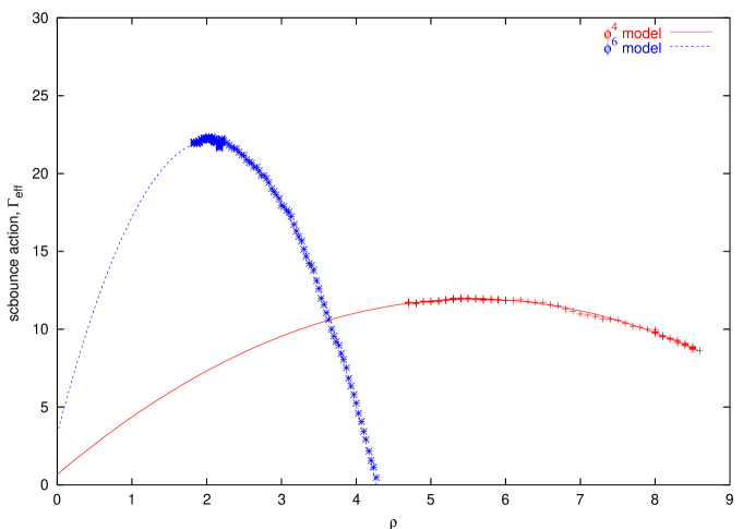
Figure 5: The self-consistent bounce action for both models is plotted as a function of the bounce radius as the bounce is dilated and contracted. The curve fits are quadratic functions and require only the location of the peak and the second derivative (curvature) as parameters.

In the self-consistent case the bubble growth instability and its translational invariance persist globally in the effective action, but are no longer manifest at the level of the fluctuation spectrum, which now consists solely of positive, “vibrational” modes. As we have alluded, translational invariance now requires simultaneous displacements of both $\phi(x)\rightarrow\phi(x+a)$ and $G(x,x)\rightarrow G(x+a,x+a)$. Similarly the bubble instability–the fact that it is a saddle point of the effective action–can be probed via a simultaneous radial dilation or contraction of both $\phi$ and $G$, see Fig. 5.

Care must be taken when tracing over the collective coordinates because the contributions from these degrees of freedom carry dimensions and potentially lead to new (infrared) divergences. The regularization of such behavior should not introduce new ad hoc scales in the calculation but rather should be consistent with the regularization and renormalization implemented in Sec. IV. In practice, the dimensionality introduced by the collective coordinates is compensated for in the transition amplitude by an infrared regulator $\mu_{0}$, which is tied to the choice of renormalization scale made above in dealing with the logarithmic divergences in the effective action tHooft . The physical (measured) mass of quasiparticles is a function of this scale $M=M(\mu_{0})$. Thus by fixing the mass in the false vacuum, we have implicitly adopted the scale choice $\mu_{0}=M_{+}$ .

We now evaluate the (consistently regularized) contribution from the collective coordinates, beginning with the translational zero modes. The effective action is invariant under a transformation which shifts the center of the bounce. As usual, the path integral obtains a factor of spacetime volume up to a Jacobian factor $J_{0}$, which in $D$ dimensions is given by

$$D[\phi(x,z)]=J_{0}d^{D}z,\qquad{\rm with}\quad J_{0}=\left[{1\over 2\pi}\int d^{D}x\left({\partial\phi_{b}\over\partial z}\right)^{2}\right]^{D/2}.$$ (69)

where the factor of $2\pi$ is conventional to make the integral commensurate with a the Gaussian case.

The integral can be expressed in terms of the effective action. To be explicit, we wish to consider the effective action now as a functional of $\phi$ alone. This amounts to the familiar transformation of the 2PI action $\Gamma_{\rm eff}[\phi,G]$ into the 1PI effective action $\Gamma^{\rm 1PI}_{\rm eff}[\phi]$, wherein $G$ is thought of as a functional of $\phi$ determined by Eq. (17) 2PI . Dividing this action into kinetic and effective potential terms, the $\phi$ equation is simply

$$-\nabla^{2}\phi+{\delta V_{\rm eff}\over\delta\phi}=0.$$ (70)

and we have essentially the same situation as in the 1-loop analysis but for the substitution of an effective potential. The argument proceeds that the effective action is conserved along a trajectory in $x$: $\partial_{x}\Gamma_{\rm eff}=0$ and its value is fixed by our choice of renormalization in the false vacuum $\Gamma_{\rm eff}[\phi_{+}]=0.$ As a consequence we can write

$${1\over 2}\left({d\phi\over dx}\right)^{2}=V_{\rm eff},\quad{\rm and}\quad J_{0}=\left[{\Gamma_{\rm eff}\over 2\pi}\right]^{D/2}.$$ (71)

The total contribution from the zero modes, together with factors of the regulator $\mu_{0}$, is

$$J_{0}\mu_{0}^{D}\int d^{D}z.$$ (72)

Next we consider what happens upon variation of the radius corresponding to the bounce solution in $\phi$ and $G$. It is convenient to shift the radial coordinate by the bounce radius, i.e. $r=R_{0}+\xi$, where $r=R_{0}$ is the radius of the bounce. Expanding the effective action around $\xi=0$ then gives

$$\Gamma_{\rm eff}\simeq\Gamma_{\rm eff}(R_{0})+\xi\Gamma^{\prime}_{\rm eff}(R_{0})+{1\over 2}\xi^{2}\Gamma^{\prime\prime}_{\rm eff}(R_{0})+\ldots$$ (73)

where primes denote radial derivatives. The first derivative of the effective action at the bounce is zero as the bounce is a solution of the equations of motion. The second derivative however is negative, as shown in Fig. 5. Just as is the case for the semiclassical solution, the self-consistent bounce is a saddle point of the effective action and a maximum in the radial “direction” (by which we mean direction in function space). The contribution of this dilatational degree of freedom to $\cal Z$ is computed in direct analogy to that of the negative mode in the 1-loop analysis, i.e. in steepest descent by continuation to imaginary $\xi$ CallanColeman . The difference is that we must now extract $\Gamma^{\prime\prime}_{\rm eff}$ by hand, so to speak, rather than from the fluctuation spectrum. Performing the integration in the radial coordinate requires again the introduction of a Jacobian

$$J_{-}=\left[{1\over 2\pi}\int d^{D}x\left({\partial\phi_{b}\over\partial R}\right)^{2}\right]^{1/2}.$$ (74)

The change to radial coordinates has no effect, and $J_{-}$ is identical to $J_{0}$ for one dimension.

The $D+1$ collective coordinates give a total multiplicative contribution to $\cal Z$ of

$${\mu_{0}}^{D+1}\left({\Gamma_{\rm eff}\over 2\pi}\right)^{D+1\over 2}\int d^{D}z\int d\xi~{}e^{-\Gamma^{\prime\prime}_{\rm eff}\xi^{2}/2},$$ (75)

or, performing the Gaussian integration,

$$\left({\Gamma_{\rm eff}\over 2\pi}\right)^{D+1\over 2}{i\mu_{0}^{D+1}\over 2}\sqrt{{2\pi\over\Gamma^{\prime\prime}_{\rm eff}}}\int d^{D}z,$$ (76)

where the factor of $1/2$ results from the analytic continuation to one branch of imaginary $\xi$ since $\Gamma^{\prime\prime}_{\rm eff}$ is negative.

Finally the rate of spontaneous decay of the false vacuum is obtained by Eq. (8),

$$\Gamma/V={\mu_{0}}^{D+1}\left[{\Gamma_{\rm eff}\over 2\pi}\right]^{D+1\over 2}\left(2\pi\over\Gamma^{\prime\prime}_{\rm eff}\right)^{1/2}~{}e^{-\Gamma{\rm eff}},$$ (77)

where all factors of $\Gamma_{\rm eff}$ and its derivatives are evaluated at the self-consistent bounce. The dimensions are correct as the factor containing derivatives of the effective action cancels one mass dimension. We present numerical results for the nucleation rate computed according to our self-consistent method described above and computed at 1-loop order in Table 2. The models are as in Eqs.(18)-(19) with parameters given by the numerical values $\mu^{2}=4.34,\lambda=0.14,\epsilon=0.67$ for the $\phi^{6}$ model and $\lambda=mu^{2}=1,\epsilon=0.12$ for the $\phi^{4}$ model.

		$\Gamma_{\rm sc}/V$		$\Gamma_{\rm 1-loop}/V$
$\phi^{4}$ model		$1.19\times 10^{-4}$		$8.59\times 10^{-3}$
$\phi^{6}$ model		$1.23\times 10^{-8}$		$1.60\times 10^{-2}$

Table 2: Numerical results for the self-consistent nucleation rate and the 1-loop rate in the two scalar models.

VII Discussion

We see that the self-consistent calculation results in a much smaller nucleation rate than the usual 1-loop estimate, from two orders of magnitude in the $\phi^{4}$ model up to six orders of magnitude for the $\phi^{6}$ model. This is a robust prediction even if the nonexponential prefactor in Eq. (77) is taken with a grain of salt. The prefactor is of the same order of magnitude in both the self-consistent and 1-loop approximations, hence it is the exponentiation of the effective action which mostly determines the magnitude of the rate. We should clarify that the “dynamical” prefactor, i.e. the ratio of fluctuation determinants in Eq. (1), is not generically of order unity. It is only the case that when the (appropriately dimensionless) determinant contribution is absorbed into the effective action in the exponent that it may be argued that the remaining prefactor is roughly determined by some mass scale typical of the problem as $M^{D}$.

The larger effective action at the self-consistent level results principally from the the shift in the spectrum (relative to 1-loop) by the fluctuation self-repulsion. The same qualitative change is observed for self-consistent topological defects, which are heavier than at 1-loop kinkpaper , and we expect it to be generically true for any self-consistently dressed quantum field configuration.

In summary, we have proposed an alternative nucleation rate computation based on a self-consistent determination of the bubble shape and fluctuation spectrum. We have traced a path analogous to the standard work of Coleman Coleman by going to imaginary time and solving instead a set of equations for the mean-field bounce and coincident two-point function obtained from a 2PI effective action. As translational invariance and bubble instability are not manifest at the level of the linearized fluctuation spectrum, we have used collective coordinates to account for the contribution of these degrees of freedom to the transition amplitude.

Finally we note that as our Euclidean spacetime solution, upon analytically continuation to Minkowski spacetime should provide a solution to the real time bubble dynamics for all time in accordance with Lorentz invariance at zero temperature stepbeyond . This is the ultimate test of whether or not what we claim above to be the self-consistent bounce (at this level of approximation) is indeed the self-consistent bounce.

Analytic continuation of the one- and two-point functions $\phi(\rho)$ and $G(\rho)$ from the last section is a straightforward matter of taking $\rho\rightarrow\sqrt{x^{2}-t^{2}}$, or at initial time $t=0$, $\rho\rightarrow|x|$. This is not however enough information to specify the real time problem. Time evolution of the coupled system of equations requires full knowledge of the spectral decomposition of $G(x,x^{\prime})$. In order to initialize these, we need to rebuild in real time the fluctuation modes that correspond to the (initially static) $\phi(x)$ and $G(x,x)$. In practice we use the methods developed in Ref. kinkpaper to easily determine the mode functions that correspond to $\phi(x)$ and $G(x,x)$ found in the previous sections. We then use them as initial conditions for the real time field evolution.

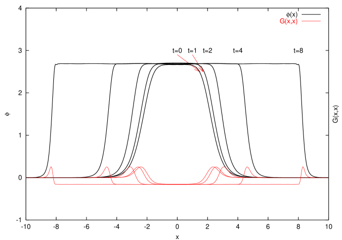
Figure 6: A stroboscopic view of the bubble growth for the self-consistent bubble of the $\phi^{6}$ model. The bubbles evolve by expansion of the true vacuum and Lorentz contraction of the walls, without giving rise to radiation, as required of the self-consistent bounce.

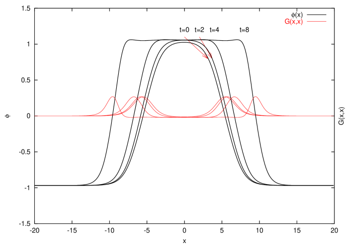
Figure 7: The same as Fig. 6 for the $\phi^{4}$ model.

At zero temperature, we should therefore observe a Lorentz invariant bubble growth without the initial transients present in the naive initializations of Ref. stepbeyond . As figures 6 and 7, corresponding to the $\phi^{6}$ and $\phi^{4}$ models, indicate the shape of the bubble is essentially unaltered during the evolution, except for Lorentz contraction.

References

- (1) J. S. Langer, Annals Phys. 41, 108 (1967) [Annals Phys. 281, 941 (2000)]. Annals Phys. 54, 258 (1969).
- (2) I. Y. Kobzarev, L. B. Okun and M. B. Voloshin, Sov. J. Nucl. Phys. 20, 644 (1975) [Yad. Fiz. 20, 1229 (1974)]. M. B. Voloshin, Yad. Fiz. 42, 1017 (1985) [Sov. J. Nucl. Phys. 42, 644 (1985)].
- (3) S. R. Coleman, Phys. Rev. D 15, 2929 (1977) [Erratum-ibid. D 16, 1248 (1977)].
- (4) C. G. Callan and S. R. Coleman, Phys. Rev. D 16, 1762 (1977).
- (5) I. Affleck, Phys. Rev. Lett. 46, 388 (1981).
- (6) A. D. Linde, Nucl. Phys. B 216, 421 (1983) [Erratum-ibid. B 223, 544 (1983)].
- (7) J. Baacke and V. G. Kiselev, Phys. Rev. D 48, 5648 (1993) J. Baacke and G. Lavrelashvili, arXiv:hep-th/0307202.
- (8) E. J. Weinberg, Phys. Rev. D 47, 4614 (1993)
- (9) A. Strumia and N. Tetradis, Nucl. Phys. B 554, 697 (1999) A. Strumia and N. Tetradis, Nucl. Phys. B 560, 482 (1999)
- (10) M. Reuter and C. Wetterich, Nucl. Phys. B 417, 181 (1994).
- (11) D. O’Connor and C. R. Stephens, Phys. Rept. 363, 425 (2002).
- (12) M. G. Alford, H. Feldman and M. Gleiser, Phys. Rev. D 47, 2168 (1993). M. G. Alford and M. Gleiser, Phys. Rev. D 48, 2838 (1993)
- (13) G. D. Moore, K. Rummukainen and A. Tranberg, JHEP 0104, 017 (2001)
- (14) The only other calculation in this spirit that we are aware of is A. Surig, Phys. Rev. D 57, 5049 (1998).
- (15) D. Boyanovsky, F. Cooper, H. J. de Vega and P. Sodano, Phys. Rev. D 58, 025007 (1998)
- (16) Y. Bergner and L. M. Bettencourt, arXiv:hep-th/0305190.
- (17) M. Salle, arXiv:hep-ph/0307080.
- (18) The relativistic formalism was developed in J. M. Cornwall, R. Jackiw and E. Tomboulis, Phys. Rev. D 10, 2428 (1974). For nonrelativistic precursors, see also J. M. Luttinger, J. C. Ward, Phys. Rev. 118 (1960) 1417; G. Baym, Phys. Rev. 127 (1962) 1391.
- (19) M. A. Lohe, Phys. Rev. D 20, 3120 (1979). This is a strictly linearized analysis. For a self-consistent quantization, see also Ref. kinkpaper .
- (20) O. J. Eboli, R. Jackiw and S. Y. Pi, Phys. Rev. D 37, 3557 (1988).
- (21) See e.g. S. Habib, Y. Kluger, E. Mottola and J. P. Paz, Phys. Rev. Lett. 76, 4660 (1996) F. Cooper, S. Habib, Y. Kluger and E. Mottola, Phys. Rev. D 55, 6471 (1997)
- (22) Y. Bergner and L. M. Bettencourt, Phys. Rev. D 68, 025014 (2003)
- (23) G. Amelino-Camelia and S. Y. Pi, Phys. Rev. D 47, 2356 (1993)
- (24) A. Rebhan and P. van Nieuwenhuizen, Nucl. Phys. B 508, 449 (1997); N. Graham and R. L. Jaffe, Phys. Lett. B 435, 145 (1998); A. Litvintsev and P. van Nieuwenhuizen, For a self-consistent analysis, see Ref. kinkpaper
- (25) We used the standard relaxation routine solvde from W. H. Press et al., Numerical recipes in Fortran 77 and Fortran 90, (Cambridge Univ. Press, Cambridge, U.K., 1996).
- (26) Specifically we used the suboutine SSGEV for radial modes with angular index which require special boundary conditions at the origin and SSTEV as appropriate elsewhere, see http://www.netlib.org/lapack/ for full reference.
- (27) W. Buchmuller, Z. Fodor, T. Helbig and D. Walliser, Annals Phys. 234, 260 (1994)
- (28) A. Kusenko, Phys. Lett. B 358, 47 (1995)
- (29) A. Kusenko, K. M. Lee and E. J. Weinberg, Phys. Rev. D 55, 4903 (1997)
- (30) D. Boyanovsky and C. Aragao de Carvalho, Phys. Rev. D 48, 5850 (1993)
- (31) G. ’t Hooft, Phys. Rev. D 14, 3432 (1976) [Erratum-ibid. D 18, 2199 (1978)].