Dynamical origin of low-mass fermions in Randall-Sundrum background

Abstract

We investigate a dynamical mechanism to generate fermion mass in the Randall-Sundrum background. We consider four-fermion interaction models where the fermion field propagates in an extra-dimension, i.e. the bulk four-fermion interaction model. It is assumed that two types of fermions with opposite parity exist in the bulk. We show that electroweak-scale mass is dynamically generated for a specific fermion anti-fermion condensation, even if all the scale parameters in the Lagrangian are set to the Planck scale.

1 Introduction

The Standard Model (SM) provides a remarkably successful description of known phenomena. On the other hand the SM has an unsatisfactory feature which is called hierarchy problem, disparity between the Planck scale and the electroweak scale. One of the solution for the hierarchy problem is found in the higher dimensional theory [1]. In the scenario the SM scale can be obtained from the ratio between the Planck scale and the size of the extra dimension.

Randall and Sundrum proposed an alternative approach to solve the hierarchy problem in a five-dimensional curved spacetime [2]. They considered the five-dimensional anti-de Sitter spacetime compactified on an orbifold, $S^{1}/Z_{2}$, and two 3-branes existing at the orbifold fixed points. The 3-branes are four-dimensional subspaces embedded in the five-dimensional spacetime. It was shown that the spacetime metric satisfies the Einstein equation and the electroweak scale $O$(TeV) is derived from the Planck scale $M_{P}$ without introducing any very large parameters.

In the beginning it is considered that the SM particles are constrained on the 3-brane. But there is a possibility the SM particles also propagate in an extra dimension, i.e. bulk SM. Goldberger and Wise pointed out that the bulk scalar fields have modes whose mass terms are exponentially suppressed on a brane as well as the brane particles [3]. We can identify the lightest modes of bulk fields to be the SM particles. There are a lot of possibilities to put the SM particles in the bulk [4, 5]. In the Randall-Sundrum background some mechanisms are proposed to generate an extremely light fermion mass like a neutrino [6].

It is the standard scenario that an elementary Higgs boson induces mass of particles through Higgs mechanism. The dynamical mass generation, for example top quark condensation [7] in extra dimensions [8], is an appealing alternative scenario. It has been known that the spacetime curvature plays an important role to dynamical symmetry breaking [9]. A four-fermion interaction model is studied in the RS background as a prototype model of dynamical symmetry breaking [10]. The dynamical origin to generate the low mass fermion is found by assuming the existence of the strong interaction between the bulk fermion and the brane fermion. Gauge theories is also considered in the RS background by using the Schwinger-Dyson equation [11]. It is pointed out that the strong interaction is naturally appears in the gauge theory. It is found that the SM scale is obtained on the brane from the bulk QCD coupled with the brane fermion.

Dynamical origin of the low mass fermion is discussed in some models with brane fermions. In the present paper we study the possibility to generate the low fermion mass dynamically starting from the theory only with the bulk fermion. Assuming the four-fermion like interaction between the bulk fermions, we evaluate the phase structure and the natural mass scale of the model. This paper is organized as follows: In section 2 we explain our setup and model. In section 3 we analyze the effective potential and fermion mass spectrums. In section 4 we make a comment on the solution for the hierarchy problem in our model. In section 5 we give the summary and discussions.

2 Bulk Four-Fermion Model

As is known, the chiral symmetry prohibits a Dirac mass term in four-dimensional spacetime. The Dirac mass term is generated through breaking of the chiral symmetry. Especially in a four-fermion model a composite operator of fermion and anti-fermion, $\bar{\psi}\psi$, may develop a non-vanishing vacuum expectation value and the chiral symmetry is broken dynamically [12]. Here we study a bulk four-fermion model in the RS spacetime. The RS spacetime is the five-dimensional spacetime which is compactified on an orbifold $S^{1}/Z_{2}$ of radius $r_{c}$.

The metric of the RS spacetime is described by

$$G_{AB}=diag(e^{-2k|y|}\eta_{\mu\nu},-1),$$

where y is the coordinate of an extra-dimensional direction. There is no chiral symmetry in the RS spacetime. To see it we consider a free bulk fermion theory,

$$S_{F}=\int d^{4}xdy\sqrt{G}\left[\bar{\psi}i\Gamma^{\bar{A}}e_{\bar{A}}^{A}(\partial_{A}+\frac{1}{8}\omega_{A}^{\bar{B}\bar{C}}[\Gamma_{\bar{B}},\Gamma_{\bar{C}}])\psi\right],$$ (1)

where $e_{\bar{A}}^{A}$ is the inverse of the vierbein and $\omega_{A}^{\bar{B}\bar{C}}$ is the spin connection. We denote the five-dimensional Dirac $\gamma$ matrix by $\Gamma_{\bar{A}}=(\gamma_{\mu},i\gamma_{5})$. The action is invariant under $y\rightarrow y\pm 2\pi r_{c}$, and therefore we can restrict y to $-\pi r_{c}<y\leq\pi r_{c}$. The action is also invariant under $y\leftrightarrow-y$. The fermion field, $\psi$, has even or odd property under five-dimensional parity transformation,

$$\left\{\begin{array}[]{l}\psi(y)\rightarrow\gamma_{5}\psi(-y)=\psi(y);even,\\ \psi(y)\rightarrow\gamma_{5}\psi(-y)=-\psi(y);odd.\\ \end{array}\right.$$ (4)

For even-parity fermion five-dimensional spinor fields can be expanded in terms of Kaluza-Klein(K-K) modes,

$$\psi(x,y) = \psi_{R}(x,y)+\psi_{L}(x,y)$$

$$= \sum_{n=0}^{\infty}\psi_{R}^{(n)}(x)g_{R}^{(n)}(y)+\psi_{L}^{(n)}(x)g_{L}^{(n)}(y).$$

The parity transformation (4) for even case gives

$$\left\{\begin{array}[]{l}g_{R}^{(n)}(y)=g_{R}^{(n)}(-y),\\ g_{L}^{(n)}(y)=-g_{L}^{(n)}(-y).\\ \end{array}\right.$$ (7)

From the periodicity on y and the latter equation of (7) we can easily see $g_{L}^{(n)}(0)=g_{L}^{(n)}(\pi r_{c})=0$. For the bases which diagonalize the Lagrangian in terms of the K-K modes, the action (1) reads

$$S_{F}=\int d^{4}x\bar{\psi}_{R}^{(0)}i\partial_{\mu}\gamma^{\mu}\psi_{R}^{(0)}+\sum_{n=1}^{\infty}\bar{\psi}^{(n)}(i\partial_{\mu}\gamma^{\mu}-m_{n})\psi^{(n)},$$

where $\psi^{(n)}=\psi_{R}^{(n)}+\psi_{L}^{(n)}$. The boundary condition $g_{L}^{(n)}(\pi r_{c})=0$ yields $m_{n}=k\pi n/(e^{k\pi r_{c}}-1)$ [4]. The properly normalized mode functions are given as follows:

$$\left\{\begin{array}[]{l}g_{R}^{(0)}=\sqrt{\frac{k}{1-e^{-k\pi r_{c}}}}e^{-\frac{1}{2}k\pi r_{c}}e^{\frac{1}{2}k|y|},\ \ g_{L}^{(0)}=0,\\ g_{R}^{(n)}=\sqrt{\frac{2k}{1-e^{-k\pi r_{c}}}}e^{-\frac{1}{2}k\pi r_{c}}e^{\frac{1}{2}k|y|}\ (n\geq 1),\\ g_{L}^{(n)}=\sqrt{\frac{2k}{1-e^{-k\pi r_{c}}}}e^{-\frac{1}{2}k\pi r_{c}}e^{\frac{1}{2}k|y|}\ (n\geq 1).\\ \end{array}\right.$$ (11)

Since $g_{L}^{(0)}=0$, only the right handed zero mode survives and other modes are vector-like. When the five-dimensional parity is odd, the spinor field is expanded as

$$\psi(x,y) = \psi_{R}(x,y)+\psi_{L}(x,y)$$

$$= \sum_{n=0}^{\infty}\psi_{R}^{(n)}(x)g_{L}^{(n)}(y)+\psi_{L}^{(n)}(x)g_{R}^{(n)}(y),$$

where the mode functions $g_{R}$ and $g_{L}$ are defined in (11).

Only one of the zero modes survives for both fermions. It is always a massless fermion because there is no chiral partners in the induced four-dimensional spacetime. We would like to pursue the scenario that chiral symmetry breaking generates the mass of fermions. To realize the chiral symmetry in four-dimensional spacetime it is necessary to introduce the five-dimensional parity even fermions in addition to the parity odd fermions as the chiral partner. It is possible that the right and left handed zero modes form the mass term via the four-fermion interaction [4].

The induced four-dimensional Lagrangian of the bulk four-fermion model is given by

$${\cal L}=\int dy\sqrt{G}[\bar{\psi}_{1}i\partial_{A}\Gamma^{A}\psi_{1}+\bar{\psi}_{2}i\partial_{A}\Gamma^{A}\psi_{2}-\hat{\lambda}(\bar{\psi}_{1}\psi_{2})(\bar{\psi}_{2}\psi_{1})],$$ (12)

where $\psi_{1}$ and $\psi_{2}$ are parity even and odd fermions respectively. Because the natural scale of bulk is the Planck scale, $M_{p}$, it is natural to take $\hat{\lambda}$  as $O(1/M_{p}^{3})$. This Lagrangian is invariant under a discrete chiral transformation;

$$\left\{\begin{array}[]{lll}\psi_{1}(x,y)&=&\gamma_{5}\psi_{1}(x,-y),\\ \psi_{2}(x,y)&=&-\gamma_{5}\psi_{2}(x,-y),\\ \end{array}\right.$$

which prohibits the mass term $m\bar{\psi_{1}}\psi_{2}$. Introducing the auxiliary field, $\sigma\sim\bar{\psi}_{1}\psi_{2}$, we rewrite the Lagrangian;

$${\cal L}=\int dy\sqrt{G}\left[\left(\begin{array}[]{cc}\bar{\psi}_{1}&\bar{\psi}_{2}\\ \end{array}\right)\left[\begin{array}[]{cc}i\partial_{A}\Gamma^{A}&-\sigma^{*}\\ \sigma&i\partial_{A}\Gamma^{A}\\ \end{array}\right]\left(\begin{array}[]{c}\psi_{1}\\ \psi_{2}\\ \end{array}\right)-\frac{|\sigma|^{2}}{\hat{\lambda}}\right].$$ (19)

After applying the K-K mode expansion the Lagrangian reads

$${\cal L} = \bar{\psi}_{1R}^{(0)}i\gamma^{\mu}\partial_{\mu}\psi_{1R}^{(0)}+\bar{\psi}_{2L}^{(0)}i\gamma^{\mu}\partial_{\mu}\psi_{2L}^{(0)}$$ (25)

$$+ \sum_{1\leq n}\left[\bar{\psi}_{1R}^{(n)}i\gamma^{\mu}\partial_{\mu}\psi_{1R}^{(n)}+\bar{\psi}_{1L}^{(n)}i\gamma^{\mu}\partial_{\mu}\psi_{1L}^{(n)}+\bar{\psi}_{2R}^{(n)}i\gamma^{\mu}\partial_{\mu}\psi_{2R}^{(n)}+\bar{\psi}_{2L}^{(n)}i\gamma^{\mu}\partial_{\mu}\psi_{2L}^{(n)}\right]$$

$$+ \sum_{0\leq m,n}\left(\begin{array}[]{cccc}\bar{\psi}_{1R}^{(m)}&\bar{\psi}_{2R}^{(m)}&\bar{\psi}_{1L}^{(m)}&\bar{\psi}_{2L}^{(m)}\\ \end{array}\right){\Large M}\left(\begin{array}[]{c}\psi_{1R}^{(n)}\\ \psi_{2R}^{(n)}\\ \psi_{1L}^{(n)}\\ \psi_{2L}^{(n)}\\ \end{array}\right)-\int dy\sqrt{G}\left[\frac{|\sigma|^{2}}{\hat{\lambda}}\right],$$

where $M$ is the fermion mass matrix which is given by

$${\Large M} = \left(\begin{array}[]{cc}0&M_{1}\\ M_{2}&0\\ \end{array}\right):$$

$$M_{1} = \left(\begin{array}[]{cc}\int\!dy\sqrt{G}[g_{R}^{(m)*}\partial_{y}g_{L}^{(n)}]&-\int\!dy\sqrt{G}[g_{R}^{(m)*}\sigma^{*}g_{R}^{(n)}]\\ -\int\!dy\sqrt{G}[g_{L}^{(m)*}\sigma g_{L}^{(n)}]&\int\!dy\sqrt{G}[g_{L}^{(m)*}\partial_{y}g_{R}^{(n)}]\\ \end{array}\right),$$

$$M_{2} = \left(\begin{array}[]{cc}-\int\!dy\sqrt{G}[g_{L}^{(m)*}\partial_{y}g_{R}^{(n)}]&-\int\!dy\sqrt{G}[g_{L}^{(m)*}\sigma^{*}g_{L}^{(n)}]\\ -\int\ dy\sqrt{G}[g_{R}^{(m)*}\sigma g_{R}^{(n)}]&-\int\!dy\sqrt{G}[g_{R}^{(m)*}\partial_{y}g_{L}^{(n)}]\\ \end{array}\right).$$

Since the RS spacetime has no translational invariance along the y direction, there appears the y dependence of vacuum expectation value, $\langle\sigma\rangle$. The vacuum expectation value $\langle\sigma\rangle$ is determined by observing the minimum of the induced four-dimensional effective potential.

3 Phase Structure in RS Background

We evaluate the induced four-dimensional effective potential and calculate the vacuum expectation value $\langle\sigma\rangle$ in the leading order of 1/N expansion. The effective four-dimensional action is derived after performing the integration over all the fermion fields,

$$S_{F}=\ln\det\left[i\partial_{\mu}\gamma^{\mu}+M[\sigma,\sigma^{*}]\right]-\int d^{4}x\int dy\sqrt{G}\left[\frac{|\sigma|^{2}}{\hat{\lambda}}\right].$$ (29)

To get the effective potential we set $\sigma$ independent of x and obtain the effective potential,

$$V_{eff}[\sigma,\sigma^{*}] = -\frac{1}{16\pi^{2}}{\rm Tr}\left[\Lambda^{4}\ln[1+\frac{M^{2}}{\Lambda^{2}}]-M^{4}\ln[1+\frac{\Lambda^{2}}{M^{2}}]+M^{2}\Lambda^{2}\right]$$ (30)

$$+ \int dy\sqrt{G}\left[\frac{|\sigma|^{2}}{\hat{\lambda}}\right]$$

with a momentum cutoff $\Lambda$, and the trace is taken over the K-K modes.

Here we restrict ourselves to the following two possibilities, $\langle\sigma\rangle=v$ and $\langle\sigma\rangle=ve^{k|y|}$. Such restricted functions may not minimize the effective potential. But note that if such functions with non-vanishing $v$ minimize the effective potential even within the restricted functions, we can see that there is more stable state than the symmetric state, $\langle\sigma\rangle=0$. In other words the chiral symmetry is broken down.

3.1 $\langle\sigma\rangle=v$ case

First we assume that the vacuum expectation value $\langle\sigma\rangle$ is independent of y, $\langle\sigma\rangle=v$. In general we cannot diagonalize the Lagrangian [25] and therefore we rely on the numerical analysis. The effective potential is expressed such that

$$V_{eff}(v)=\frac{v^{2}}{\lambda}-\frac{1}{16\pi^{2}}{\rm Tr}\left[\Lambda^{4}\ln[1+\frac{M(v)^{2}}{\Lambda^{2}}]-M(v)^{4}\ln[1+\frac{\Lambda^{2}}{M(v)^{2}}]+M(v)^{2}\Lambda^{2}\right].$$

Here $M(v)$ is a matrix whose components are $M_{mn}(0\leq m,n\leq 2N_{KK})$ with

$$M_{00} = \frac{v}{a}\ln[1+a],$$

$$M_{0n} = M_{n0}=\frac{\sqrt{2}v}{a}\left[\cos[\frac{n\pi}{a}]\left\{C_{i}(\frac{n\pi(1+a)}{a})-C_{i}(\frac{n\pi}{a})\right\}\right.$$

$$\left.+\sin[\frac{n\pi}{a}]\left\{S_{i}(\frac{n\pi(1+a)}{a})-S_{i}(\frac{n\pi}{a})\right\}\right]\ \ \ (1\leq n\leq N_{KK}),$$

$$M_{0n} = M_{n0}=0\ \ \ (N_{KK}+1\leq n\leq 2N_{KK}),$$

$$M_{mn} = \frac{v}{a}\left[\cos[\frac{(m+n)\pi}{a}]\left\{C_{i}(\frac{(m+n)\pi(1+a)}{a})-C_{i}(\frac{(m+n)\pi}{a})\right\}\right.$$

$$\left.+\sin[\frac{(m+n)\pi}{a}]\left\{S_{i}(\frac{(m+n)\pi(1+a)}{a})-S_{i}(\frac{(m+n)\pi}{a})\right\}\right.$$

$$\left.+\cos[\frac{(m-n)\pi}{a}]\left\{C_{i}(\frac{(m-n)\pi(1+a)}{a})-C_{i}(\frac{(m-n)\pi}{a})\right\}\right.$$

$$\left.+\sin[\frac{(m-n)\pi}{a}]\left\{S_{i}(\frac{(m-n)\pi(1+a)}{a})-S_{i}(\frac{(m-n)\pi}{a})\right\}\right]$$

$$(1\leq m,n\leq N_{KK}),$$

$$M_{mn} = M_{nm}=m_{n}\delta_{m,n}\ \ \ (1\leq m\leq N_{KK},N_{KK}+1\leq n\leq 2N_{KK}),$$

$$M_{mn} = \frac{v}{a}\left[\cos[\frac{(m-n)\pi}{a}]\left\{C_{i}(\frac{(m-n)\pi(1+a)}{a})-C_{i}(\frac{(m-n)\pi}{a})\right\}\right.$$

$$\left.+\sin[\frac{(m-n)\pi}{a}]\left\{S_{i}(\frac{(m-n)\pi(1+a)}{a})-S_{i}(\frac{(m-n)\pi}{a})\right\}\right.$$

$$\left.-\cos[\frac{(m+n-2N_{KK})\pi}{a}]\left\{C_{i}(\frac{(m+n-2N_{KK})\pi(1+a)}{a})-C_{i}(\frac{(m+n-2N_{KK})\pi}{a})\right\}\right.$$

$$\left.-\sin[\frac{(m+n-2N_{KK})\pi}{a}]\left\{S_{i}(\frac{(m+n-2N_{KK})\pi(1+a)}{a})-S_{i}(\frac{(m+n-2N_{KK})\pi}{a})\right\}\right]$$

$$\ \ \ (N_{KK}+1\leq m,n\leq 2N_{KK}),$$

where $a=e^{k\pi r_{c}}-1,m_{n}=nk\pi/a$ and $\lambda=4k\hat{\lambda}/(1-e^{-4k\pi r_{c}})$, and $C_{i}$ and $S_{i}$ are the cosine-integral and sine-integral function respectively. We take $N_{KK}$ as $a\frac{k\pi}{\Lambda}+1$ such that we neglect K-K modes heavier than $\Lambda$ in the unbroken phase.

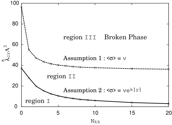
For small $N_{KK}$ we can calculate the effective potential numerically. Through numerical inspections we find that the chiral symmetry is broken down at a critical coupling. The phase transition from the symmetric phase to the broken phase is of the second order. In Fig. 1 we draw the critical coupling constant by the dotted line against $N_{KK}$ as $k=\Lambda=M_{P}$ fixed.

3.2 $\langle\sigma\rangle=ve^{k|y|}$ case

Next we consider the case, $\langle\sigma\rangle=ve^{k|y|}$. In this case we easily diagonalize the mass term and perform the y integration in Eq. (25). The Lagrangian reduces to

$${\cal L} = \frac{1}{\lambda}v^{2}+\left(\begin{array}[]{cc}\bar{\psi}_{1R}^{(0)}&\bar{\psi}_{2L}^{(0)}\\ \end{array}\right)\left(\begin{array}[]{cc}i\gamma^{\mu}\partial_{\mu}&-v\\ -v&i\gamma^{\mu}\partial_{\mu}\\ \end{array}\right)\left(\begin{array}[]{c}\psi_{1R}^{(0)}\\ \psi_{2L}^{(0)}\\ \end{array}\right)$$ (49)

$$+\sum_{n\geq 1}\left(\begin{array}[]{c}\bar{\psi}_{1R}^{(n)}\\ \bar{\psi}_{2R}^{(n)}\\ \bar{\psi}_{1L}^{(n)}\\ \bar{\psi}_{2L}^{(n)}\\ \end{array}\right)^{T}\left(\begin{array}[]{cc|cc}i\partial_{\mu}\gamma^{\mu}&0&m_{n}&-v\\ 0&i\partial_{\mu}\gamma^{\mu}&-v&m_{n}\\ \hline\cr m_{n}&-v&i\partial_{\mu}\gamma^{\mu}&0\\ -v&m_{n}&0&i\partial_{\mu}\gamma^{\mu}\end{array}\right)\left(\begin{array}[]{c}\psi_{1R}^{(n)}\\ \psi_{2R}^{(n)}\\ \psi_{1L}^{(n)}\\ \psi_{2L}^{(n)}\\ \end{array}\right),$$

where $\lambda$ is $2k\hat{\lambda}/(1-e^{-2k\pi r_{c}})$ and $m_{n}=nk\pi/(e^{k\pi r_{c}}-1)$. Fermion mass matrix $M$ has the following form,

$$M=\left(\begin{array}[]{cc}0&\begin{array}[]{ll}m_{n}&-v\\ -v&M_{n}\\ \end{array}\\ \begin{array}[]{ll}m_{n}&-v\\ -v&M_{n}\\ \end{array}&0\\ \end{array}\right).$$

The mass of the fermion is given by the eigen value of $M$, i.e. $v$ and $|v\pm\frac{nk\pi}{a}|$.

In the leading order of the $1/N$ expansion the effective potential for the Lagrangian (49) is given by

$$V_{eff}=\frac{1}{\lambda}v^{2}-\frac{1}{16\pi^{2}}\left[\Lambda^{4}\ln\left[1+\frac{v^{2}}{\Lambda^{2}}\right]-v^{4}\ln\left[1+\frac{\Lambda^{2}}{v^{2}}\right]+v^{2}\Lambda^{2}\right]$$

$$-\frac{1}{16\pi^{2}}\sum_{n<N_{KK}}\left[\Lambda^{4}\ln\left[1+\frac{v_{+}^{2}}{\Lambda^{2}}\right]-v_{+}^{4}\ln\left[1+\frac{\Lambda^{2}}{v_{+}^{2}}\right]+v_{+}^{2}\Lambda^{2}\right.$$

$$\left.+\Lambda^{4}\ln\left[1+\frac{v_{-}^{2}}{\Lambda^{2}}\right]-v_{-}^{4}\ln\left[1+\frac{\Lambda^{2}}{v_{-}^{2}}\right]+v_{-}^{2}\Lambda^{2}\right],$$ (53)

where we define that $v_{+}\equiv v+\frac{nk\pi}{a},v_{-}\equiv v-\frac{nk\pi}{a}$. Differentiating the effective potential by $v^{2}$ we obtain the gap equation;

$$\frac{\partial^{2}}{\partial v^{2}}V_{eff}(v) = \frac{2}{\lambda}-\frac{1}{4\pi^{2}}\left[1+\frac{2v^{2}}{1+v^{2}}-3v^{2}\ln\left[1+\frac{1}{v^{2}}\right]\right]$$

$$-\frac{1}{4\pi^{2}}\sum_{n\leq N_{KK}} \left[2+\frac{2v_{+}^{2}}{1+v_{+}^{2}}-3v_{+}^{2}\ln\left[1+\frac{1}{v_{+}^{2}}\right]+\frac{2v_{-}^{2}}{1+v_{-}^{2}}-3v_{-}^{2}\ln\left[1+\frac{1}{v_{-}^{2}}\right]\right]$$

$$= 0.$$

For each numerical value of the coupling constant $\lambda$ we calculate the effective potential (53). It is found that the second order phase transition takes place, and the chiral symmetry is broken down above the critical value of the coupling constant. The critical coupling constant, $\hat{\lambda}_{cr}$, is obtained by solving the equation; $[\partial^{2}/\partial v^{2}\ \ V_{eff}(v)]_{v=0}=0,$

$$\lambda_{cr}=8\pi^{2}\left[1+\sum_{n\leq N_{KK}}\left\{2+\frac{4(nk\pi)^{2}}{a^{2}+(nk\pi)^{2}}-6(\frac{nk\pi}{a}^{2})\ln[\frac{a^{2}+(nk\pi)^{2}}{(nk\pi)^{2}}]\right\}^{-1}\right].$$ (54)

Figure 1: Critical coupling constant

In Fig. 1 we show the critical coupling constant by the solid line against $N_{KK}$ as $k=\Lambda=M_{P}$ fixed. In the region $II$ and $III$ the chiral symmetry is broken. The most remarkable feature shows up in the region $II$. In this region the y-dependent state is more stable than the y-independent state.

4 Natural Mass Scale

What is the natural mass scale for the lightest fermion in the bulk four-fermion model? Only a mass scale in the bulk is the Planck scale, $M_{P}$. We take all the mass scale in the bulk as $O(M_{P})$, i.e. $k\simeq\Lambda\simeq M_{P}$ and set $kr_{c}\simeq 12$, which gives $N_{KK}\simeq 10^{16}$. For such a large $N_{KK}$ the critical coupling (54) behaves to be inverse proportional to $N_{KK}$ in the $\langle\sigma\rangle=ve^{ky}$ case,

$$\hat{\lambda}_{cr}\rightarrow\frac{2\pi^{2}}{(1-\ln 2)k^{2}\Lambda N_{KK}}\simeq\frac{20}{\Lambda^{3}}e^{-k\pi r_{c}},$$

which is much smaller than the natural scale $1/M_{p}^{3}$.

For $\langle\sigma\rangle=v$ case the critical coupling constant behaves almost like a constant value, $\hat{\lambda}_{cr}\Lambda\simeq O(30)$, in our numerical analysis, Fig. 1. It is larger than the natural scale. Therefore we conclude that the four-fermion coupling at the natural scale, $\hat{\lambda}\simeq\ 1/M_{P}^{3}$, is located in the region $II$ in Fig. 1. In this region the effective potential for $\langle\sigma\rangle=ve^{ky}$ is smaller than the y-independent vacuum. If the y-dependent vacuum, $\langle\sigma\rangle\simeq ve^{ky}$, is a true vacuum of the theory, the mass of fermions is given by $v,|v\pm\pi/a|$. One of the fermion necessarily has mass below $\pi/a\sim O(M_{EW})$ independently of the value $v$. Thus the lightest fermion mass is generated dynamically at the electroweak scale, $k\pi/a$, even if the vacuum expectation value $v$ is at the Planck scale $M_{P}$. A low mass fermion exists in the bulk four fermion model. It is one of the dynamical realizations of the RS mechanism [11, 13].

5 Summary and Discussion

We have investigated the bulk four-fermion model in the RS spacetime. We assume the existence of two kinds of bulk fermions with different parity. It is necessary to introduce the chiral symmetry in the induced four-dimensional model. The effective potential is calculated in the induced model. Evaluating the minimum of the effective potential we found that the extra direction y-dependent vacuum is more stable than the y-independent one for a special region of the coupling constant. If we take all the mass scale in the bulk as the Planck scale, the lightest fermion mass is generated dynamically at the electroweak scale. Therefore a low mass fermion is obtained in our model. It shows the possibility to build up a realistic model which may solve the hierarchy problem dynamically in the RS spacetime.

In the present analysis we restrict ourselves to the special form for the y-dependence of the vacuum expectation value. Our solution may not be the true minimum of the effective potential. To find a true minimum of the effective potential we calculate the effective potential (30) for a general y-dependent $\langle\sigma\rangle$. It is interesting to calculate the stress tensor in our model and solve the Einstein equation. The y-dependent $\langle\sigma\rangle$ naturally change the spacetime structure.

In the RS spacetime there are two 3-branes at the orbifold fixed point, $y=0$ and $y=\pi r$. The radiative correction of the brane fields has something to do with the vacuum expectation value. But the mass scale of the $y=\pi r$ brane is the electroweak scale, $M_{EW}$. Since the influence of the brane fields is of the order $O(M_{EW})$, the mass scale of the lightest fermion keeps at the electroweak scale.

A SUSY extension of our model is also interesting. We have two kinds of fermion in our model. In the RS spacetime we can construct N=2 SUSY model, which include two kinds of fermions automatically [14].

References

• [1] I. Antoniadis, Phys. Lett. B 246, 377 (1990);
N. Arkani-Hamed, S. Dimopoulos, and G. Dvali, Phys. Lett. B429, 263 (1998); Phys. Rev. D59, 086004 (1999).
• [2] L. Randall, R. Sundrum, Phys. Rev. Lett. 83, 3370 (1999).
• [3] W. D. Goldberger and M. B. Wise, Phys. Rev. Lett. 83, 4922 (1999).
• [4] S. Chang, J. Hisano, H. Nakano, N. Okada, M. Yamaguchi, Phys. Rev. D62, 084025 (2000).
• [5] H. Davoudiasl, J. L. Hewett, T. G. Rizzo, Phys. Rev. D63, 075004 (2001).
• [6] Y. Grossman, M. Neubert, Phys. Lett. B474, 361 (2000);
N. Arkani-Hamed, S. Dimopoulos, G. R. Dvali, J. March-Russell, Phys. Rev. D65, 024032 (2002).
• [7] V. A. Miransky, M. Tanabashi and K. Yamawaki, Phys. Lett. B221, 177 (1989); Mod. Phys. Lett. A4, 1043 (1989);
C. T. Hill and E. H. Simmons, Phys. Rept. 381, 235 (2003).
• [8] B. A. Dobrescu, Phys. Lett. B461, 99 (1999);
H. Cheng, B. A. Dobrescu and C. T. Hill, Nucl. Phys. B 589, 249 (2000);
N. Arkani-Hamed, H. Cheng, B. A. Dobrescu and L. J. Hall, Phys. Rev. D62, 096006 (2000);
H. Abe, H. Miguchi and T. Muta, Mod. Phys. Lett. A15, 445 (2000);
A. B. Kobakhidze, Phys. Atom. Nucl. 64, 941 (2001) [Yad.Β Fiz.Β  64, 1010 (2001)];
M. Hashimoto, M. Tanabashi and K. Yamawaki, Phys. Rev. D64, 056003 (2001); hep-ph/0304109; V. Gusynin, M. Hashimoto, M. Tanabashi and K. Yamawaki, Phys. Rev. D65, 116008 (2002);
• [9] T. Inagaki, T. Muta and S. D. Odintsov, Mod. Phys. Lett. A8 2117 (1993); Prog. Theor. Phys. Suppl. 127 93 (1997);
E. Elizalde, S. D. Odintsov and Yu. I. Shilnov, Mod. Phys. Lett. A9, 913 (1994);
T. Inagaki, S. Mukaigawa and T. Muta, Phys. Rev. D52, 4267 (1995);
K. Ishikawa, T. Inagaki and T. Muta, Mod. Phys. Lett. A11, 939 (1996);
T. Inagaki, Int. J. Mod. Phys. A11 4561 (1996).
• [10] H. Abe, T. Inagaki, T. Muta, in Fluctuating Paths and Fields, edited by W. Janke, A. Pelster, H.-J. Schmidt, and M. Bachmann (World Scientific, Singapore, 2001);
N. Rius, V. Sanz, Phys. Rev. D64, 075006 (2001).
• [11] H. Abe, T. Inagaki, Phys. Rev. D66, 085001 (2002);
H. Abe, K. Fukazawa, and T. Inagaki, Prog. Theor. Phys. 107, 1047 (2002);
H. Abe, hep-ph/0307004.
• [12] Y. Nambu and G. Jona-Lasinio, Phys. Rev. 122, 345 (1961).
• [13] L. Randall, R. Sundrum, Phys. Rev. Lett. 83, 4690 (1999);
H. Davoudiasl, J. L. Hewett, T. G. Rizzo, Phys. Rev. Lett. 84, 2080 (2000); Phys. Lett. B473, 43 (2000).
• [14] I. L. Buchbinder, T. Inagaki and S. D. Odintsov, Mod. Phys. Lett. A12, 2271 (1997);
T. Inagaki, S. D. Odintsov and Y. I. Shil’nov, Int. J. Mod. Phys. A14, 481 (1999).