hep-ph/0307397
OSU-HEP-03-11

MCTP-03-38

FERMILAB-Pub-03/222

August 2003

Test of Gauge-Yukawa Unification
Ilia Gogoladze,^a Yukihiro Mimura,^b S. Nandi^a,c and Kazuhiro Tobe^d

^aDepartment of Physics, Oklahoma State University, Stillwater, OK 74078-3072
^bDepartment of Physics, University of Regina, Regina, SK, S4S 0A2, Canada
^cFermi National Accelerator Laboratory, PO Box 500, Batavia, IL 60510
^dMCTP, Department of Physics, University of Michigan, Ann Arbor, MI 48109
^dDepartment of Physics, University of California, Davis, CA 95616

Recently it has been proposed that, in the framework of quantum field theory, both the Standard Model gauge and Yukawa interactions arise from a single gauge interaction in higher dimensions with supersymmetry. This leads to the unification of the Standard Model gauge couplings and the third family Yukawa couplings at the GUT scale. In this work, we make a detailed study of this unification using the current experimental data, and find a good agreement in a significant region of the parameter space. Similar relations, required in Finite Grand Unification models, are also studied.

1 Introduction

Standard Model (SM), based on the gauge symmetry group, $SU(3)_{C}\times SU(2)_{L}\times U(1)_{Y}$, has been very successful experimentally. There is still no evidence beyond SM, except possibly the neutrino masses and mixings. However, SM has many parameters, such as three gauge couplings, $g_{3}$, $g_{2}$ and $g_{1}$ and many Yukawa couplings such as $y_{t}$, $y_{b}$, $y_{\tau}$, $y_{c}$, $y_{s}$, $y_{\mu}$, $y_{u}$, $y_{d}$, $y_{e}$ (where $y_{t}$ denotes the Yukawa coupling of the top quark to the SM Higgs boson and so on), mixing angles and phases. It will be nice to relate some of these parameters using symmetry. Grand Unification Theory (GUT) such as $SU(5)$, $SO(10)$ or $E_{6}$ relates the gauge couplings, since all the gauge interactions of the SM arise from the single gauge interaction of the unifying group. This gives $g_{3}=g_{2}=g_{1}$ at the unification scale, $M_{GUT}$, leading to the successful prediction for the $\sin^{2}\theta_{W}$ at low energy in supersymmetric (SUSY) GUT. For specific choices of the Higgs sector, GUT can also relates some of the Yukawa couplings. For example, in $SU(5)$ theory, we can have $y_{b}=y_{\tau}$, where in $SO(10)$, we can have $y_{t}=y_{b}=y_{\tau}$ at the GUT scale. Such GUT relations among the Yukawa coupling also lead to successful prediction at the low energy for a significant region of the SUSY parameter space. (For recent progress for top-bottom-tau Yukawa unification, see Refs. [1, 2, 3, 4, 5, 6].)

One interesting fact we have observed is that in a scenario of top-bottom-tau Yukawa unification together with gauge coupling unification at the GUT scale, the unified Yukawa coupling ($y_{G}$) can be very close to the unified gauge coupling ($g_{G}$) ($g_{G}\simeq 0.7$ and $y_{G}\geq 0.5$) in a wide range of parameter space. This fact interestingly implies that the origin of Yukawa couplings might be related to the unified gauge coupling. Therefore it naturally leads us to consider an interesting possibility of “gauge-Yukawa unification” at high-energy scale. In this work, we will study the numerical test of such possibility. We consider two different models in which gauge and Yukawa couplings are related. One is the higher dimensional model, and the other is so-called finite GUT model.

In higher dimensional models, the Yukawa interactions can be just part of the gauge interactions. If we go to higher dimensions, the higher dimensional components of the gauge bosons (say $A_{5},A_{6},\cdots$) are scalar fields, and can be identified with the Higgs bosons [7, 8, 9, 10]. The higher dimensional fermions include both chiral two-component spinors in the four dimensional (4D) language. By orbifolding condition, the resulting 4D theories can be chiral [11]. The higher dimensional kinetic term of the fermion includes the Dirac-type mass term of the Kaluza-Klein excited modes such as $\overline{\Psi_{L}}\partial_{5}\Psi_{R}$. The extra dimensional derivative $\partial_{5}$ must be gauge covariant due to the gauge invariance, and thus the lagrangian has the Yukawa term such as $\overline{\Psi_{L}}A_{5}\Psi_{R}$. Therefore, if the Higgs fields which break electroweak symmetry are unified to the gauge bosons in higher dimensions and the quarks and leptons are zero-modes of the higher dimensional fermions, the Yukawa interaction in the SM is just part of the gauge interactions. In non-SUSY models, we need at least 6D to unify the standard model Higgs fields with the higher dimensional components of gauge bosons. The reason we cannot realize the unification in 5D is that we need, at least, two real components to identify the higher dimensional components of the gauge fields with Higgs fields. In SUSY models, we can construct gauge-Higgs unified models in 5D [8]. The 5D N=1 SUSY model corresponds to 4D N=2 SUSY. The N=2 gauge multiplet includes N=1 chiral superfield $\Sigma$ (the imaginary part of its scalar components is $A_{5}$), and we can identify the part of $\Sigma$ with the Higgs field. In this model, thus, the Yukawa couplings can originate from the gauge interaction. We can also construct gauge-Higgs unified models in 6D N=2 SUSY [9, 10] which corresponds to 4D N=4 SUSY. The N=4 gauge multiplet contains N=1 vector multiplet and three chiral superfields. In the models of Ref. [10], gauge fields, Higgs bosons as well as the third family matter fermions are unified in a single multiplet belonging to the adjoint representation of the unified gauge group in 6D. In this way both the Yukawa and the gauge interactions, in the compactified 4D theory, arise from a single gauge interaction in 6D, and thus the gauge and third family Yukawa couplings are unified at the compactification scale. The smallness of the first- and second-family Yukawa couplings can be realized by using the volume suppression, fermion localization [12], Froggatt-Nielsen like mechanism [13], and so on.

The object of this work is to perform a detailed analysis of such unification of the gauge couplings ($g_{1}$, $g_{2}$, $g_{3}$) and the third family Yukawa couplings ($y_{t}$, $y_{b}$, $y_{\tau}$) within the framework of SUSY models. We find that a significant region of the parameter space allow such an unification with the key prediction for $\tan\beta$ ($\tan\beta\simeq$ 52) and the correlation among SUSY threshold corrections at low energy.  Therefore, precise measurement of SUSY parameters in future experiments will be quite important to test this prediction of the gauge-Yukawa unification.

The relations between the Yukawa couplings and gauge couplings have also been found at the finite GUT models [15, 16], which are four-dimensional models. Though such relations do not arise from a symmetry, imposition of such relations at the GUT scale lead to the finite GUT models, thus reducing the number of parameters in the theory. In this work, we also investigate how well such finite GUT relations work, and again find a good agreement for a significant region of the parameter space.

2 Formalism

2.1 Gauge-Yukawa unification

A model realizing the unification of the gauge couplings ($g_{1}$, $g_{2}$, $g_{3}$) and the third family Yukawa couplings ($y_{t}$, $y_{b}$, $y_{\tau}$) was presented in [10]. It has an $SU(8)$ gauge symmetry in 6D with N=2 SUSY. N=2 SUSY in 6D corresponds to N=4 SUSY in 4D, thus only the gauge multiplet can be introduced in the bulk. 6D N=2 gauge multiplet, expressed in terms of 4D, N=4 gauge multiplet, contains the vector multiplet $V(A_{\mu},\lambda)$ and three chiral multiplets in the adjoint (63-dimensional) representation of the gauge group. The 63-dimensional gauge multiplet contains the gauge bosons (and their superpartners) while the three 63-dimensional chiral multiplets contain the third family matter fermions and the Higgs bosons plus their superpartners. Two extra dimensions are compactified in $T^{2}/Z_{6}$ orbifold. With suitable choice of the $Z_{6}$ transformation matrix, $SU(8)$ is broken to the $SU(4)\times SU(2)_{L}\times SU(2)_{R}\times U(1)^{2}$, and the theory reduces to 4D N=1 SUSY Pati-Salam model with two extra $U(1)$ symmetry. The massless modes after compactification are the Pati-Salam gauge fields, $\mathbf{(15,1,1),(1,3,1),(1,1,3)}$ plus two additional singlet vector fields $\mathbf{(1,1,1)}$ and $\mathbf{(1,1,1)}$, third-family matter fermions $\Psi_{L}=\mathbf{(4,\,2,\,1)}_{2,\,0}$ and $\Psi_{\bar{R}}=\mathbf{(\bar{4},\,1,\,2)}_{-2,\,-4}$ and bi-doublet Higgs fields, $H_{1}=\mathbf{(1,\,2,\,2)}_{0,\,4}$ and $H_{2}=\mathbf{(1,\,2,\,2)}_{0,\,-4}$. Since all the fields are contained in one representation of one simple gauge symmetry (63-dimensional representation of $SU(8)$ in 6D in this case), all interactions in this theory arises only from gauge interaction. The trilinear coupling for the chiral multiplets

$$S=\int d^{6}x\left[\int d^{2}\theta\,2\,{\rm Tr}\left(-\sqrt{2}g_{6}\Sigma[\Phi,\Phi^{c}]\right)+h.c.\right]$$ (1)

includes the Yukawa interaction terms

$$S=\int d^{6}x\int d^{2}\theta\,y_{6}{\Psi}_{L}H_{1}\Psi_{\bar{R}}+h.c.$$ (2)

In Eq. (1), $\Sigma,\,\Phi,\,\Phi^{c}$ are chiral multiplets containing the third family chiral fields, $\Psi_{L}$ and $\Psi_{\bar{R}}$, and the bi-doublet Higgs fields, $H_{1}$ and $H_{2}$, and $g_{6}$ and $y_{6}$ are the 6D gauge and Yukawa couplings. Eqs. (1) and (2) leads to $g_{6}=y_{6}$ with proper kinetic normalization. Integrating out the two extra dimensions, we obtain $y_{4}=g_{4}$ for the 4D coupling leading to

$$g_{1}=g_{2}=g_{3}=y_{t}=y_{b}=y_{\tau}(=y_{\nu_{\tau}}^{\rm Dirac})$$ (3)

at the compactification scale ($M_{c}$) which is also the unification scale in our theory. We assume that the Pati-Salam symmetry, as well as the two extra $U(1)$ are broken at $M_{c}$ to the $SU(3)_{c}\times SU(2)_{L}\times U(1)_{Y}$ using suitable Higgs fields at the brane so that the particle spectrum below $M_{c}$ is the same as in MSSM. This model is one concrete example which predicts the relation (3). The 6D N=2 SUSY $SU(8)$ model can be modified to 6D N=2 SUSY $SO(16)$ [10], and many other models can be constructed with different low energy symmetry, but all having gauge-Yukawa unification [17]. The relation (3) is the gauge and Yukawa unification for the third family, whose validity and phenomenological implication will be tested in the next section.

2.2 Finite GUT unification

Another possibility to connect the Gauge and the Yukawa couplings is finite N=1 SUSY theory [15, 16] wherein the $\beta$-functions for the gauge and the Yukawa couplings vanish to all orders in perturbation theory. In order to have all loop finite theory, there is definite set of conditions which need to be satisfied. Below we briefly review these conditions .

The one-loop gauge and Yukawa $\beta$-functions and the one-loop anomalous dimension of the matter fields in a generic SUSY Yang-Mills theory are given by [18]:

$$\beta^{(1)}_{g} = \frac{g^{3}}{16\pi^{2}}\left(\sum_{R}T(R)-3C_{2}(G)\right),$$ (4)

$$\beta^{(1)}_{ijk} = \lambda_{ijp}\gamma^{(1)}{}^{p}_{k}+(k\leftrightarrow i)+(k\leftrightarrow j),$$ (5)

$$\gamma^{(1)}{}^{i}_{j} = \frac{1}{16\pi^{2}}[\lambda^{ikl}\lambda_{jkl}-2C_{2}(R)g^{2}\delta^{i}_{j}],$$ (6)

where $T(R)$, $C_{2}(R)$ and $C_{2}(G)$ are the Dynkin indices for the matter fields and the quadratic Casimirs for the matter and gauge representations respectively. $\lambda^{ijk}$ and $\beta^{(1)}_{ijk}$ are the Yukawa couplings and the one-loop Yukawa $\beta$-functions of $\lambda^{ijk}$. The criteria of all loop finiteness for N=1 SUSY gauge theories can be stated as follows [19]:

(I) It should be free from gauge anomaly.

(II) The gauge $\beta$-function vanishes at one loop: $\beta^{(1)}_{g}=0$.

(III) There exists solution of the form $\lambda=\lambda(g)$ for the conditions of vanishing one-loop anomalous dimensions: $\gamma^{(1)}{}^{i}_{j}=0$.

(IV) The solution is isolated and non-degenerate when considered as a solution of vanishing one-loop Yukawa $\beta$-function: $\beta^{(1)}_{ijk}=0$.
If all four conditions are satisfied, the dimensionless parameters of the theory would depend on a single gauge coupling constant and the $\beta$-functions will vanish to all orders.

Models satisfying the criteria (I) through (IV) have been found in the $SU(5)$ SUSY GUT [15, 16] with appropriate particle contents. One such solution [16] relating the gauge and the third family Yukawa couplings based $SU(5)\times A_{4}$ symmetry is

$$y_{b}=y_{\tau}=\frac{\sqrt{3}}{2}y_{t}={\frac{3}{\sqrt{10}}}g_{G}\,,$$ (7)

where $A_{4}$ is the group of even permutation [20], $y_{t}$, $y_{b}$ and $y_{\tau}$ are the top, bottom and tau Yukawa couplings, and $g_{G}$ is the gauge coupling at the unification scale.

3 Analysis of gauge-Yukawa unification scenarios

In this section, we analyze two gauge-Yukawa unification scenarios in which Yukawa couplings can be related to the unified gauge coupling: “gauge-Yukawa unification ($y_{t}=y_{b}=y_{\tau}=g_{G}$)” and “finite-GUT unification”. It has been stressed that high-energy Yukawa couplings are highly sensitive to low-energy SUSY threshold corrections to Yukawa and gauge couplings especially in large $\tan\beta$ case. Therefore, in a study of any Yukawa unification scenarios, an inclusion of low-energy SUSY threshold corrections is very important. Following the analysis done in Ref. [3], we perform a semi-SUSY model-independent analysis to see if the gauge-Yukawa unification scenarios are realistic or not. In our analysis, we use a dimensional reduction ($\overline{\rm DR}$) renormalization scheme, which is known to be consistent with SUSY. ${\overline{\rm{DR}}}$ Yukawa couplings ($y_{t,b,\tau}$) and gauge couplings ($g_{i}$) in the MSSM at Z-boson mass scale are written as follows:

$${y}_{t}(m_{Z}) = \frac{\sqrt{2}\bar{m}_{t}^{\rm{MSSM}}(m_{Z})}{\bar{v}(m_{Z})\sin\beta}=\frac{\sqrt{2}\bar{m}_{t}^{\rm{SM}}(m_{Z})}{\bar{v}(m_{Z})\sin\beta}\left(1+\delta_{t}\right),$$ (8)

$${y}_{b,\tau}(m_{Z}) = \frac{\sqrt{2}\bar{m}_{b,\tau}^{\rm{MSSM}}(m_{Z})}{\bar{v}(m_{Z})\cos\beta}=\frac{\sqrt{2}\bar{m}_{b,\tau}^{\rm{SM}}(m_{Z})}{\bar{v}(m_{Z})\cos\beta}\left(1+\delta_{b,\tau}\right),$$ (9)

$${g}_{i}(m_{Z}) = \bar{g}_{i}^{\rm{SM}}(m_{Z})\left(1+\delta_{g_{i}}\right),~{}~{}(i=1-3)$$ (10)

where $\bar{m}_{i}^{\rm{SM}}$ and $\bar{g}_{i}^{\rm{SM}}$ are $\overline{\rm{DR}}$ quantities defined in the SM, and $\bar{v}$ and $\tan\beta$ are $\overline{\rm DR}$ values in the MSSM. They are determined following the analysis in Ref. [3]. (See Ref. [3] for detail and references.) Especially when we calculate $\bar{m}_{i}^{\rm{SM}}(m_{Z})$, we adopt top pole mass ($m_{t}=174.3\pm 5.1$ GeV), tau pole mass ($m_{\tau}=1776.99^{+0.29}_{-0.26}$ MeV) and $\overline{\rm{MS}}$ bottom mass ($\bar{m}^{\rm MS}_{b}(\bar{m}^{\rm MS}_{b})=4.26\pm 0.30$ GeV). The quantities $\delta_{t,b,\tau,g_{i}}$ represent SUSY threshold corrections. If we choose a certain SUSY breaking scenario, they are fixed. In our analysis, however, we treat them as free parameters without specifying any particular SUSY breaking scenario.

When all parameters $\delta_{t,b,\tau,g_{i}}$ are specified, all $\overline{\rm{DR}}$ couplings in the MSSM are determined at $m_{Z}$. Then we use two-loop renormalization group equations (RGEs) for the MSSM couplings in order to study the unification of couplings at the GUT scale. Requiring a certain unification scenario, we can obtain constraints among parameters $\delta_{t,b,\tau,g_{i}}$, as we will see later. In this paper, we assume that the theory between $m_{Z}$ and the GUT scale is well described by the MSSM.

3.1 Gauge-Yukawa unification $y_{t}=y_{b}=y_{\tau}=g_{G}$

Here we consider a possibility that all SM gauge couplings, top, bottom and tau Yukawa couplings are unified at the GUT scale, which we call “gauge-Yukawa unification” ($y_{t}=y_{b}=y_{\tau}=g_{G}$). In order to study the gauge-Yukawa unification, first we look for a region where top, bottom and tau Yukawa couplings are unified ($y_{t}=y_{b}=y_{\tau}\equiv y_{G}$) at the GUT scale. We define the GUT scale ($M_{G}$) as a scale where $g_{1}(M_{G})=g_{2}(M_{G})\equiv g_{G}$. In our analysis, we allow the possibility that the strong gauge coupling is not exactly unified: $g_{3}(M_{G})^{2}/g_{G}^{2}=1+\epsilon_{3}$ where $\epsilon_{3}$ can be a few %. This mismatch $\epsilon_{3}$ from exact unification can be considered to be due to a GUT scale threshold correction to the unified gauge coupling.

In Fig. 1, contours of $\delta_{b}$ (dotted lines in Fig. (a)), $\tan\beta$ (dashed lines in Fig. (b)) and $\epsilon_{3}$ (dotted lines in Fig. (b)) are shown as a function of $\delta_{t}$ and $\delta_{g_{3}}$, which are required for the Yukawa unification ($y_{t}=y_{b}=y_{\tau}$) at the GUT scale. In Fig. 1, we take central values of input fermion masses ($m_{t}=174.3$ GeV, $\bar{m}_{b}^{\rm MS}(\bar{m}_{b}^{\rm MS})=4.26$ GeV and $m_{\tau}=1776.99$ MeV) and $\delta_{\tau}=0.02$. In order to fix $\delta_{g_{1,2}}$, we assume that all SUSY mass parameters which contribute to $\delta_{g_{1,2}}$ are equal to $500$ GeV ($\delta_{g_{1}}=-0.006$ and $\delta_{g_{2}}=-0.02$). As shown in Fig. 1, $\tan\beta$ should be about $50$, and the value of $\delta_{b}$ should be a few % [2, 3], which is much smaller than one naively expected in large $\tan\beta$ case [21].

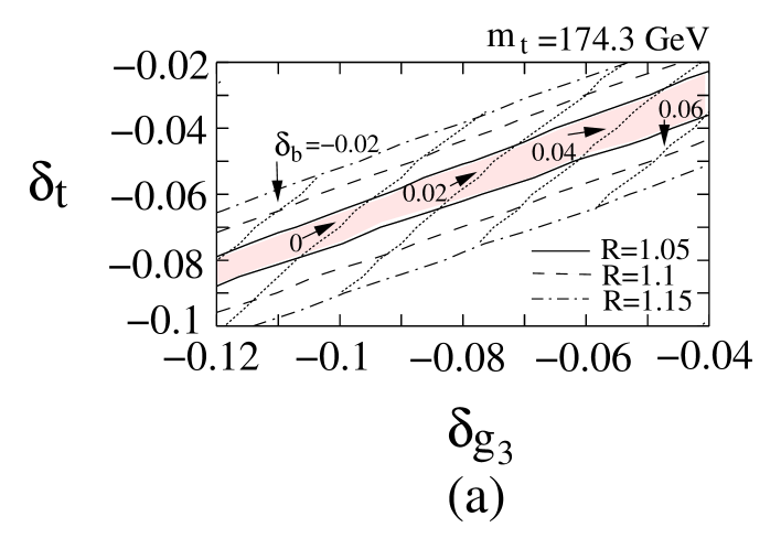
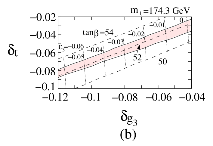
Figure 1: Parameter space satisfying the gauge-Yukawa unification. Contours of $\delta_{b}$ (dotted lines in Fig. (a)), $\tan\beta$ (dashed lines in Fig. (b)) and $\epsilon_{3}$ (dotted lines in Fig. (b)) are shown as a function of $\delta_{t}$ and $\delta_{g_{3}}$, required for Yukawa unification ($y_{t}=y_{b}=y_{\tau}$). After finding the region for the Yukawa unification, contours of a parameter $R$ (defined in text) are plotted in Fig. (a). The shaded regions represent a region where the gauge-Yukawa unification is achieved within $5\%$ level ($R\leq 1.05$). Here we have fixed $m_{t}=174.3$ GeV, $\bar{m}^{\rm MS}_{b}(\bar{m}^{\rm MS}_{b})=4.26$ GeV, $m_{\tau}=1776.99$ MeV, $\delta_{\tau}=0.02$, $\delta_{g_{1}}=-0.006$ and $\delta_{g_{2}}=-0.02$.

Our next question is: “Is there any region where the unified Yukawa coupling ($y_{G}$) is really unified into the unified gauge coupling ($g_{G}$)?” After requiring Yukawa unification, we calculate a parameter $R$ defined as follows:

$$R \equiv \frac{{\rm max}(y_{t},y_{b},y_{\tau},g_{1},g_{2},g_{3})}{{\rm min}(y_{t},y_{b},y_{\tau},g_{1},g_{2},g_{3})}\simeq\left\{\begin{array}[]{c}y_{G}/g_{G}~{}~{}{\rm for}~{}~{}y_{G}>g_{G},\\ g_{G}/y_{G}~{}~{}{\rm for}~{}~{}y_{G}<g_{G}.\end{array}\right.$$ (13)

When $R=1$, exact gauge-Yukawa unification happens. In Fig. 1(a), contours of $R$ are shown to see if there is a region in which the gauge-Yukawa unification happens. As one can see from Fig. 1(a), there is a region where the gauge-Yukawa unification is well achieved. In the shaded regions of Fig. 1, the gauge-Yukawa unification is realized within $5\%$ level ($R\leq 1.05$) allowing $\epsilon_{3}$ to be a few %. Note that the gauge-Yukawa unification requires an interesting relation between $\delta_{t}$ and $\delta_{g_{3}}$ and a very specific $\tan\beta$ ($\tan\beta\simeq 52$) in addition to small $\delta_{b}$. We have checked that the value of $\epsilon_{3}$ is quite sensitive to values of $\delta_{g_{1,2}}$ because a change of $\delta_{g_{1,2}}$ shifts the unified gauge coupling $g_{G}$ but not $g_{3}(M_{G})$ very much. On the other hand, the relation between $\delta_{t}$ and $\delta_{g_{3}}$ as well as the value of $\tan\beta$ does not depend on $\delta_{g_{1,2}}$ very much. Therefore we have found that the relation between $\delta_{t}$ and $\delta_{g_{3}}$ and the values of $\tan\beta$ ($\tan\beta\simeq 52$) are rather stable predictions from the gauge-Yukawa unification. Thus in principle, if SUSY parameters were measured precisely enough to know $\delta_{t}$, $\delta_{g_{3}}$ and $\tan\beta$, the gauge-Yukawa unification could be tested.

In the above analysis, we have fixed top and bottom masses. We note that a change of top (bottom) mass simply shifts an allowed region of parameter $\delta_{t}$ ($\delta_{b}$). For example, if we take $m_{t}$ to be $174.3+5.1$ ($\simeq 174.3(1+0.03)$) GeV, the allowed region of $\delta_{t}$ is shifted by about $-0.03$. Since uncertainties of top and bottom masses are still large, the precise determination of these masses is also quite important to test the gauge-Yukawa unification.

We comment on some possible high-energy threshold corrections. One possible correction would be due to neutrino Yukawa couplings. If neutrino Yukawa couplings are large and run below the GUT scale, they induce at most a few % corrections to GUT-scale Yukawa couplings. As a result, the effects modify the value of the unified Yukawa coupling and the relation among the SUSY threshold correction parameters by a few %, as discussed in Ref. [3]. Other possible corrections could originate from the theory of extra-dimensions [22]. There would be corrections from the brane localized interactions. These corrections can be negligible if the volume of extra dimensions is large. Also there might be some corrections from the integration of extra-dimensions. These corrections, however, highly depend on the nature of extra-dimensions (number of extra-dimensions and SUSY, topology of extra-dimensions etc). Therefore, we will not try to discuss the model-dependent corrections. Instead, we can see some effects to the allowed region for the gauge-Yukawa unification, adopting the parameter $R$. We have plotted contours of $R$ in Fig. 1(a). These contours show how much the allowed region can change if a deviation from $R=1$ originates from these high-energy threshold corrections. As can be seen, if the deviation is of the order of a few %, still the allowed region is well constrained. In the discussions in section 4, we will assume that the gauge-Yukawa unification is realized within 5% ($R\leq 1.05$) to see the implication of the gauge-Yukawa unification.

3.2 Finite GUT unification

In this section, we consider another type of gauge-Yukawa unification. In a model discussed in Ref. [15, 16], the finiteness condition implies the unification at the GUT scale given by Eq. (7). This provides an interesting relation between Yukawa and gauge couplings at the GUT scale, and we call it “finite GUT unification”.

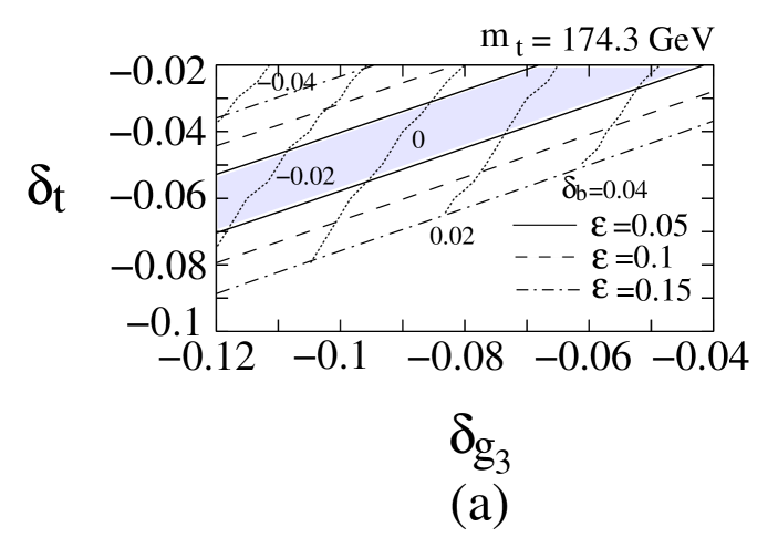
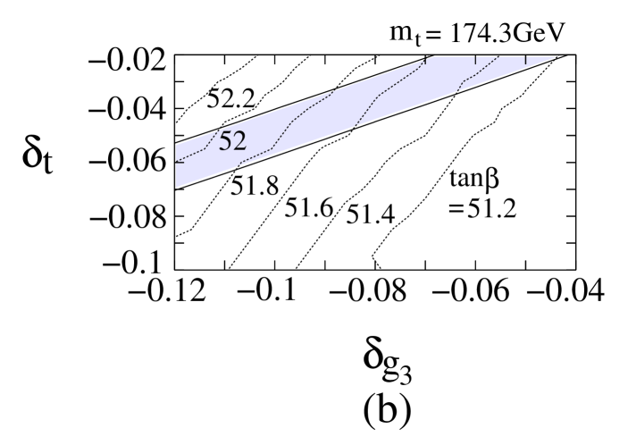
Figure 2: Parameter space satisfying the finite GUT unification. Contours of $\delta_{b}$ (dotted lines in Fig. (a)) and $\tan\beta$ (dotted lines in Fig. (b)) are shown as a function of $\delta_{t}$ and $\delta_{g_{3}}$, required for bottom-tau-gauge unification ($y_{b}=y_{\tau}=g_{G}\sqrt{9/10}$). After finding the bottom-tau-gauge unification, we also plot contours of $\epsilon$ (defined in text) in Fig. (a). The shaded regions represent a region in which the finite GUT gauge-Yukawa unification is achieved within 5% level ($\epsilon\leq 0.05$). Here we have fixed $m_{t}=174.3$ GeV, $\bar{m}^{\rm MS}_{b}(\bar{m}^{\rm MS}_{b})=4.26$ GeV, $m_{\tau}=1776.99$ MeV, $\delta_{\tau}=0.02$, $\delta_{g_{1}}=-0.006$ and $\delta_{g_{2}}=-0.02$.

In order to find an allowed region for the finite GUT unification, we first search for a region where bottom, tau and gauge coupling unification in Eq. (7) ($y_{b}=y_{\tau}=\sqrt{9/10}g_{G}$) happens. In Fig. 2, we show relations among parameters $\delta_{t}$, $\delta_{g_{3}}$, $\delta_{b}$ and $\tan\beta$ which are required for the bottom-tau-gauge unification in Eq. (7). Contours of $\delta_{b}$ (dotted lines in Fig. (a)) and $\tan\beta$ (dotted lines in Fig. (b)) are shown as a function of $\delta_{t}$ and $\delta_{g_{3}}$. Here we have taken central values of input fermion masses, and $\delta_{\tau}=0.02$, $\delta_{g_{1}}=-0.006$, $\delta_{g_{2}}=-0.02$. Similar to the gauge-Yukawa unification discussed in the previous section, $\delta_{b}$ is required to be small, and $\tan\beta$ should be around 50.

Then we look for a region in which top and gauge coupling unification in Eq. (7) ($y_{t}=g_{G}\sqrt{6/5}$) is realized after finding the bottom-tau-gauge unification in Eq.(7). We define a parameter $\epsilon$:

$$\epsilon=\frac{\left|y_{t}-g_{G}\sqrt{6/5}\right|}{y_{t}},$$ (14)

so that $\epsilon=0$ if the finite GUT unification Eq. (7) is achieved. In Fig. 2(a), we plot contours of $\epsilon$. As can be seen from Fig. 2, we found a region where the finite GUT unification is realized. The shaded regions in Fig. 2 represent a region where the finite GUT gauge-Yukawa unification is achieved within 5% level ($\epsilon\leq 0.05$).

Notice that the finite GUT gauge-Yukawa unification constrains SUSY threshold correction parameters $\delta_{t,b,\tau,g_{i}}$. Especially, it requires a correlation between $\delta_{t}$ and $\delta_{g_{3}}$, which interestingly suggests a slightly different relation from the one for the gauge-Yukawa unification discussed in the previous section.

In the next section, we discuss the implication of the relations between $\delta_{t}$ and $\delta_{g_{3}}$ to SUSY mass spectrum.

4 Implications to superparticle mass spectrum

We have analyzed two different gauge-Yukawa unification scenarios. Each scenario predicts a certain relation between $\delta_{t}$ and $\delta_{g_{3}}$. It is interesting to discuss implications of these relations to superparticle mass spectrum.

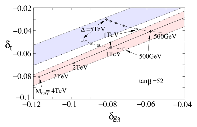
Figure 3: Relations between $\delta_{t}$ and $\delta_{g_{3}}$. In the solid line, all SUSY mass parameters are set to be equal to $M_{\rm SUSY}$, then the relation between $\delta_{t}$ and $\delta_{g_{3}}$ is shown as a function of $M_{\rm SUSY}$. In the dashed and dash-dotted lines, all the first and second generation squarks, wino and bino masses are assumed to be equal to $\Delta$ and the rest of SUSY masses to be $M_{\rm SUSY}$. In the dashed (dash-dotted) line, the relation between $\delta_{t}$ and $\delta_{g_{3}}$ is shown for $M_{\rm SUSY}=1$ TeV ($M_{\rm SUSY}=500$ GeV) as a function of $\Delta$. Two shaded regions represent the allowed regions for “gauge-Yukawa unification” ($R\leq 1.05$) in lower shaded region and for “finite GUT unification” ($\epsilon\leq 0.05$) in upper shaded region. Here we have fixed $m_{t}=174.3$ GeV, $\bar{m}^{\rm MS}_{b}(\bar{m}^{\rm MS}_{b})=4.26$ GeV, $m_{\tau}=1776.99$ MeV and $\tan\beta=52$.

If all SUSY mass parameters (gaugino masses $M_{g_{i}}$, sfermion masses $m_{\tilde{f}}$, and $\mu$-term) are simply set to be equal to $M_{\rm SUSY}$, and A-term is set to be zero, and then we calculate $\delta_{t}$ and $\delta_{g_{3}}$ as a function of $M_{\rm SUSY}$, we get a relation between $\delta_{t}$ and $\delta_{g_{3}}$ as shown in Fig. 3 (solid line). Here we have assumed $m_{t}=174.3$ GeV, $\bar{m}_{b}^{\rm MS}(\bar{m}_{b}^{\rm MS})=4.26$ GeV, $m_{\tau}=1776.99$ MeV and $\tan\beta=52$. We also show points for $M_{\rm SUSY}=500$ GeV, 1, 2, 3 and 4 TeV on the solid line in Fig. 3. One can see that as $M_{\rm SUSY}$ gets larger, both $\delta_{t}$ and $\delta_{g_{3}}$ become smaller. In Fig. 3, two shaded regions represent the allowed regions for “gauge-Yukawa unification” (lower shaded region) and for “finite GUT unification” (upper shaded region) obtained in the previous section. As can be seen from Fig. 3, interestingly the solid line just lies on the allowed region for the gauge-Yukawa unification. This choice of SUSY mass parameters is one example to realize the relation between $\delta_{t}$ and $\delta_{g_{3}}$ suggested by the gauge-Yukawa unification. Therefore, getting the relation predicted by the gauge-Yukawa unification is not particularly difficult.

At given $\delta_{t}$, the finite GUT unification requires smaller $\delta_{g_{3}}$ than one for the gauge-Yukawa unification. Note that all colored SUSY particles contribute to $\delta_{g_{3}}$, on the other hand, only the third generation squarks as well as gauginos and higgsinos contribute to $\delta_{t}$. Thus it is suggested that the finite GUT unification prefers the heavier first and second generation squarks more than the gauge-Yukawa unification does. This is an interesting implication from two different gauge-Yukawa unification scenarios.

We assume that all the first and second-generation squark masses, wino and bino masses are equal to $\Delta$, and the rest of SUSY parameters stays at $M_{\rm SUSY}$. Then we show how the relation between $\delta_{t}$ and $\delta_{g_{3}}$ changes as a function of $\Delta$ in Fig. 3. Dashed line is for $M_{\rm SUSY}=1$ TeV, and dash-dotted line for $M_{\rm SUSY}=500$ GeV. We also show points for $\Delta=500$ GeV, 1, 2, 3, 4 and 5 TeV on both dashed and dash-dotted lines in Fig. 3. One can see that clearly rather heavy first and second generation squarks are preferred for the finite GUT unification.

In order to realize the gauge-Yukawa unification, one needs to satisfy one more constraint on $\delta_{b}$. To get small $\delta_{b}$, a cancellation or a suppression among contributions to $\delta_{b}$ is needed as discussed in Ref. [2, 3]. Therefore, keeping the relation between $\delta_{t}$ and $\delta_{g_{3}}$, we need to tune parameters such as stop, sbottom, gluino, chargino masses and A-term to get the required $\delta_{b}$. For example, in a case with $M_{\rm SUSY}=\Delta=500$ GeV (1 TeV) in Fig. 3 for the gauge-Yukawa unification, we need $M_{\tilde{g}_{3}}=500$ GeV (1 TeV), $m_{\tilde{Q}_{3}}=m_{\tilde{t}_{R}}=200$ GeV ($400$ GeV), $m_{\tilde{b}_{R}}=1500$ GeV (3 TeV), $\mu=100$ GeV and $A_{t}=0.45M_{\rm SUSY}$ ($0.4M_{\rm SUSY}$) to obtain small $\delta_{b}$ ($\delta_{b}\sim 0.04$ ($0.03$)) keeping the relation between $\delta_{t}$ and $\delta_{g_{3}}$. Because of the relation between $\delta_{t}$ and $\delta_{g_{3}}$ and the constraint on $\delta_{b}$ predicted by the gauge-Yukawa unification, SUSY mass parameters have to be highly correlated. As realistic examples, we have noticed that in the supergravity-type SUSY breaking scenario, data point 1 on Table 1 in the second paper of Ref. [2] and data points 1–3 in Ref. [6] are explicit cases for the gauge-Yukawa unification. Therefore, there exists a model which realizes the gauge-Yukawa unification as well as provides the observed relic density of dark matter and a good fit to precision electroweak data. 

Since the gauge-Yukawa unification scenarios require the correlation among SUSY mass parameters, precise measurement of the SUSY parameters will be important and necessary in order to probe the gauge-Yukawa unifications.

References

- [1] H. Baer, M. A. Diaz, J. Ferrandis and X. Tata, Phys. Rev. D 61, 111701 (2000) [hep-ph/9907211]; H. Baer and J. Ferrandis, Phys. Rev. Lett. 87, 211803 (2001) [hep-ph/0106352].
- [2] T. Blazek, R. Dermisek and S. Raby, Phys. Rev. Lett. 88, 111804 (2002) [hep-ph/0107097]; Phys. Rev. D 65, 115004 (2002) [hep-ph/0201081].
- [3] K. Tobe and J. D. Wells, Nucl. Phys. B 663, 123 (2003) [hep-ph/0301015].
- [4] D. Auto, H. Baer, C. Balazs, A. Belyaev, J. Ferrandis and X. Tata, JHEP 0306, 023 (2003) [hep-ph/0302155].
- [5] C. Balazs and R. Dermisek, JHEP 0306, 024 (2003) [hep-ph/0303161].
- [6] R. Dermisek, S. Raby, L. Roszkowski and R. Ruiz De Austri, JHEP 0304, 037 (2003) [hep-ph/0304101].
- [7] N. S. Manton, Nucl. Phys. B 158, 141 (1979); D. B. Fairlie, J. Phys. G 5, L55 (1979); Phys. Lett. B 82, 97 (1979); P. Forgacs and N. S. Manton, Commun. Math. Phys. 72, 15 (1980); G. Chapline and R. Slansky, Nucl. Phys. B 209, 461 (1982); S. Randjbar-Daemi, A. Salam and J. Strathdee, Nucl. Phys. B 214, 491 (1983); I. Antoniadis, Phys. Lett. B 246, 377 (1990); N. V. Krasnikov, Phys. Lett. B 273, 246 (1991); D. Kapetanakis and G. Zoupanos, Phys. Rept. 219, 1 (1992); I. Antoniadis and K. Benakli, Phys. Lett. B 326, 69 (1994) [hep-th/9310151]; H. Hatanaka, T. Inami and C. S. Lim, Mod. Phys. Lett. A 13, 2601 (1998) [hep-th/9805067]. G. R. Dvali, S. Randjbar-Daemi and R. Tabbash, Phys. Rev. D 65, 064021 (2002) [hep-ph/0102307]; N. Arkani-Hamed, A. G. Cohen and H. Georgi, Phys. Lett. B 513, 232 (2001) [hep-ph/0105239]; L. J. Hall, H. Murayama and Y. Nomura, Nucl. Phys. B 645, 85 (2002) [hep-th/0107245]; I. Antoniadis, K. Benakli and M. Quiros, New J. Phys. 3, 20 (2001) [hep-th/0108005]; C. Csaki, C. Grojean and H. Murayama, Phys. Rev. D 67, 085012 (2003) [hep-ph/0210133]; G. von Gersdorff, N. Irges and M. Quiros, Nucl. Phys. B 635, 127 (2002) [hep-th/0204223]; arXiv:hep-ph/0206029; C. A. Scrucca, M. Serone and L. Silvestrini, arXiv:hep-ph/0304220.
- [8] G. Burdman and Y. Nomura, Nucl. Phys. B 656, 3 (2003) [hep-ph/0210257]; N. Haba and Y. Shimizu, Phys. Rev. D 67, 095001 (2003) [hep-ph/0212166]; I. Gogoladze, Y. Mimura and S. Nandi, Phys. Lett. B 560, 204 (2003) [hep-ph/0301014].
- [9] L. J. Hall, Y. Nomura and D. R. Smith, Nucl. Phys. B 639, 307 (2002) [hep-ph/0107331].
- [10] I. Gogoladze, Y. Mimura and S. Nandi, Phys. Lett. B 562, 307 (2003) [hep-ph/0302176]; arXiv:hep-ph/0304118.
- [11] P. Candelas, G. T. Horowitz, A. Strominger and E. Witten, Nucl. Phys. B 258, 46 (1985); L. J. Dixon, J. A. Harvey, C. Vafa and E. Witten, Nucl. Phys. B 261, 678 (1985).
- [12] N. Arkani-Hamed and M. Schmaltz, Phys. Rev. D 61, 033005 (2000) [hep-ph/9903417]; E. A. Mirabelli and M. Schmaltz, Phys. Rev. D 61, 113011 (2000) [hep-ph/9912265]; D. E. Kaplan and T. M. Tait, JHEP 0111, 051 (2001) [hep-ph/0110126].
- [13] C. D. Froggatt and H. B. Nielsen, Nucl. Phys. B 147, 277 (1979).
- [14] J. L. Chkareuli and I. G. Gogoladze, Phys. Rev. D 58, 055011 (1998) [hep-ph/9803335].
- [15] D. Kapetanakis, M. Mondragon and G. Zoupanos, Z. Phys. C 60, 181 (1993) [hep-ph/9210218]; J. Kubo, M. Mondragon and G. Zoupanos, Nucl. Phys. B 424, 291 (1994); J. Kubo, M. Mondragon, N. D. Tracas and G. Zoupanos, Phys. Lett. B 342, 155 (1995) [hep-th/9409003]; J. Kubo, M. Mondragon and G. Zoupanos, Acta Phys. Polon. B 27, 3911 (1997) [hep-ph/9703289].
- [16] K. S. Babu, T. Enkhbat and I. Gogoladze, Phys. Lett. B 555, 238 (2003) [hep-ph/0204246]; K. S. Babu, T. Kobayashi and J. Kubo, Phys. Rev. D 67, 075018 (2003) [hep-ph/0212350].
- [17] I. Gogoladze, Y. Mimura and S. Nandi, in preparation.
- [18] A. J. Parkes and P. C. West, Nucl. Phys. B 256, 340 (1985); D. R. Jones and A. J. Parkes, Phys. Lett. B 160, 267 (1985); D. R. Jones and L. Mezincescu, Phys. Lett. B 136, 242 (1984); Phys. Lett. B 138, 293 (1984).
- [19] C. Lucchesi, O. Piguet and K. Sibold, Helv. Phys. Acta 61, 321 (1988); Phys. Lett. B 201, 241 (1988); C. Lucchesi and G. Zoupanos, Fortsch. Phys. 45, 129 (1997) [hep-ph/9604216].
- [20] E. Ma and G. Rajasekaran, Phys. Rev. D 64, 113012 (2001) [hep-ph/0106291].
- [21] R. Hempfling, Phys. Rev. D 49, 6168 (1994); L. J. Hall, R. Rattazzi and U. Sarid, Phys. Rev. D 50, 7048 (1994) [hep-ph/9306309]; M. Carena, M. Olechowski, S. Pokorski and C. E. Wagner, Nucl. Phys. B 426, 269 (1994) [hep-ph/9402253]; R. Rattazzi and U. Sarid, Phys. Rev. D 53, 1553 (1996) [hep-ph/9505428]; D. M. Pierce, J. A. Bagger, K. T. Matchev and R. j. Zhang, Nucl. Phys. B 491, 3 (1997) [hep-ph/9606211].
- [22] Z. Kakushadze and T. R. Taylor, Nucl. Phys. B 562, 78 (1999) [hep-th/9905137]; L. J. Hall and Y. Nomura, Phys. Rev. D 65, 125012 (2002) [hep-ph/0111068]; A. Hebecker and A. Westphal, Annals Phys. 305, 119 (2003) [hep-ph/0212175].