Scaling Rule for Nonperturbative Radiation in a Class of Event Shapes

Abstract:

We discuss nonperturbative radiation for a recently introduced class of infrared safe event shape weights, which describe the narrow-jet limit. Starting from next-to-leading logarithmic (NLL) resummation, we derive an approximate scaling rule that relates the nonperturbative shape functions for these weights to the shape function for the thrust. We argue that the scaling reflects the boost invariance implicit in NLL resummation, and discuss its limitations. In the absence of data analysis for the new event shapes, we compare these predictions to the output of the event generator PYTHIA.

1 Introduction

The hadronic final states of hard-scattering reactions encode information about the full range of QCD dynamics, from the short-distance production of quarks and gluons reflected in jet production, to the long-time process of hadronization reflected in the exclusive distributions of particles in the final state. Event shapes [1, 2, 3, 4], which generalize jet cross sections, are functions of final-state momenta that measure the flow of energy [5]. We refer to these functions as ‘weights’ below. Event shape weights are tools with which we may analyze the long distance behavior of QCD through jet events. Qualitatively, we expect that cross sections for states with narrow, low-mass jets are sensitive to long-distance dynamics, while more inclusive cross sections, dominated by higher-mass jets, are predicted more accurately by perturbation theory. By varying the values of event shape weights we may select narrow or wide jet events, and thus vary the relative importance of long- and short-distance dynamics.

Infrared safe event shapes are those that are well-defined order by order in perturbation theory. For the mean values of such event shapes, or for values of the weight where higher order perturbative corrections are relatively small, nonperturbative effects enter as additive power corrections. The analysis of perturbation theory suggests that these are typically integer powers of $1/Q$, with $Q$ the overall center of mass (c.m.) energy in annihilation processes or the momentum transfer in deep-inelastic scattering [6, 7, 8, 9, 10, 11, 12]. The universality properties of power corrections, also inferred from perturbation theory, can be used to provide measurements of the strong coupling [13, 14]. As we approach the narrow jet limit, however, perturbative cross sections generically develop large logarithmic corrections.

When the weights of event shapes are symmetric in the phase space of final state particles, their large logarithmic corrections may be resummed in the limit of narrow jets, to next-to-leading logarithm (NLL) [15, 16, 17] and beyond [18] in $\rm e^{+}e^{-}$ annihilation. The analogous but even more challenging analysis has been carried out for jet events in deep-inelastic scattering [19, 20]. For many such quantities in $\rm e^{+}e^{-}$ annihilation, it is possible to factorize perturbative and nonperturbative corrections in a well-defined fashion [21], and to study the latter phenomenologically.

Familiar examples include the thrust, $T$ [1], jet broadening, $B$ [3], and the heavy jet mass, $\rho_{H}$ [4]. Short distance effects are treated in resummed perturbation theory and control the leading-power behavior in $Q$ including logarithms [15, 16, 17, 18]. Long-distance effects still enter as power corrections, whose form may be inferred from perturbation theory in a manner analogous to power corrections to the mean values of event shapes [8, 9]. An example is $1-T$, with $T$ the thrust in $\rm e^{+}e^{-}$ annihilation, for which the first power correction near $T=1$ is $1/[(1-T)Q]$. This correction grows rapidly as $T\rightarrow 1$, but it exponentiates [8, 9]. The effect is to shift the perturbative distribution [8, 9], which allows additional determinations of the strong coupling in conjunction with nonperturbative parameters [14]. For small $1-T$, not only the first power correction, but all corrections of the form $1/[(1-T)Q]^{n}$ may be organized into shape functions [21, 22] in a manner that we will review below.

Considerable progress has been made in determining shape functions for the thrust, C-parameter and heavy jet mass [23, 24, 25, 26, 27]. It is clearly desirable, however, to widen the class of event shapes to allow systematic studies of the approach to nonperturbative dynamics in infrared safe observables.

In this paper, we attempt to pursue such an approach, using the class of event shapes introduced in [18], which includes the thrust and jet broadening as special cases. As in [18], we will restrict ourselves to event shapes that vanish in the two-jet limit for $\rm e^{+}e^{-}$ annihilation, but extensions to quantities that probe multi-jet structure are possible [28], and we will discuss the differences briefly below.

We will follow Refs. [8, 9, 21] in deducing the form of power corrections from the resummed event shape weights at next-to-leading logarithm [18] in terms of shape functions. For the class of weights that we consider, we will identify an approximate scaling relation for their nonperturbative shape functions. We argue that this scaling reflects the boost invariance of the underlying soft dynamics. We will work for the most part directly in a transform space, where the resummation of large perturbative as well as power corrections is most transparent.

Because we know of no experimental data analysis for this class of observables, we compare the predictions of our scaling rule to the event generator PYTHIA [29]. As we shall see, PYTHIA reproduces the scaling over a range of parameters. We will briefly discuss the dynamical effects that are neglected in the derivation of our scaling law, and what we may conclude from the event generator results.

The following section reintroduces the event shapes of Ref. [18], and in Section 3 we review their resummation, including their numerical evaluation in perturbation theory, following the methods of Refs. [15, 16]. We derive the scaling rule and describe its interpretation in terms of boost invariance in Section 4. In Section 5 we discuss its comparison with PYTHIA [29] for shifts in the distribution peaks and for moments of the shape functions. We close with a summary. A brief appendix gives some details on the evaluation of integrals for the resummed distributions.

2 The Class of Event Shapes

We consider final states $N$ characterized by two nearly back-to-back jets,

$$e^{+}+e^{-}\rightarrow J_{1}(N)+J_{2}(N)\,,$$ (1)

at center of mass energy $Q\gg\Lambda_{\mbox{\tiny QCD}}$. For each such final state, a thrust axis is determined as the unit vector $\hat{n}$ that maximizes the the thrust $T$ [1]:

$$T(N)=\max\limits_{\hat{n}}\frac{\sum\limits_{{\rm all}\ i\in N}\left|\vec{p}_{i}\cdot\hat{n}\right|}{\sum\limits_{{\rm all}\ j\in N}\left|\vec{p}_{j}\right|}\,.$$ (2)

The class of event shapes $\tau_{a}$ of Ref. [18] is defined in terms of this axis. Parameter $a$ is adjustable, $-\infty<a<2$, and allows us to study various event shapes within the same formalism. It helps to control the approach to the two-jet limit.

The weight functions defined in Ref. [18] for a state $N$ are

$$\tau_{a}(N)={1\over Q}\sum_{{\rm all}\ i\in N}\ \omega_{i}\,\left(\sin\theta_{i}\right)^{a}\,\left(1-|\cos\theta_{i}|\right)^{1-a}\,,$$ (3)

in terms of particle energies $\omega_{i}$ and the angles $\theta_{i}$ of the particle momenta to the thrust axis. For the discussion below, we will find it more convenient to introduce a form directly in terms of particle momenta,

$$\tau_{a}(N)={1\over Q}\sum_{{\rm all}\ i\in N}\ p_{i\;T}\;e^{-|\eta_{i}|(1-a)}\,,$$ (4)

where $p_{i\;T}$ is the transverse momentum relative to the thrust axis, and $\eta_{i}$ is the corresponding pseudorapidity,

$$\eta_{i}=\ln\cot\left(\theta_{i}/2\right)\,.$$ (5)

The case $a=0$ in Eq. (4) is essentially $1-T$, with $T$ the thrust while $a=1$ is the jet broadening. A similar weight function with a non-integer power has been discussed in a related context for $2>a>1$ in [7]. The two forms for the weight functions, Eqs. (3) and (4) are equivalent for massless particles. We will use (4), in terms of momenta and pseudorapidities, in the analysis of nonperturbative corrections below. We will recall later the difference between the two forms of the event shapes when applied to massive hadrons [30].

Any choice $a<2$ in (4) specifies an infrared safe event shape variable, because the contribution of any particle $i$ to the event shape behaves as $\theta_{i}{}^{2-a}$ in the collinear limit, $\theta_{i}=\cos^{-1}|\hat{n}_{i}\cdot\hat{n}|\rightarrow 0$. However, the resummed formula given below from Ref. [18] is valid only for $a<1$. For $a\geq 1$ recoil effects have to be taken into account, at least beyond the level of leading logarithm [17]. As $a\rightarrow 2$ the weight vanishes only very slowly for $\theta_{i}\rightarrow 0$, and at fixed $\tau_{a}$, the jets become very narrow. On the other hand, the limit $a\rightarrow-\infty$ corresponds to the total cross section.

The differential cross section for such dijet events at fixed values of $\tau_{a}$ is given by

$${d\sigma(\tau_{a},Q)\over d\tau_{a}} = {1\over 2Q^{2}}\ \sum_{N}\;|M(N)|^{2}\,\delta(\tau_{a}-\tau_{a}(N)),$$ (6)

where we sum over all final states $N$ that contribute to the weighted event, and where $M(N)$ denotes the corresponding amplitude for ${\rm e^{+}e^{-}}\rightarrow N$.

Since we are investigating two-jet cross sections, we fix the constant $\tau_{a}$ to be much less than unity:

$$0<\tau_{a}\ll 1\,.$$ (7)

For small $\tau_{a}$, the cross section (6) has corrections in $\ln(1/\tau_{a})$, which have been organized in Ref. [18]. In the following we will quote the result of the resummation of large logarithms of $\tau_{a}$ in Laplace moment space. The Laplace transform of the cross section (6) is given by

$$\tilde{\sigma}\left(\nu,Q,a\right) = \int^{1}_{0}d\tau_{a}\,{\rm e}^{\;-\nu\,\tau_{a}}\ {d\sigma(\tau_{a},Q)\over d\tau_{a}}\,.$$ (8)

Logarithms of $1/\tau_{a}$ are transformed to logarithms of $\nu$. For large $\nu$, dependence on the upper limit in the $\tau_{a}$ integral is exponentially suppressed. Here and below quantities with tildes are the transforms in $\tau_{a}$, and quantities without tildes denote untransformed functions. Our results below are valid in the region where $\ln\nu$ is much larger than $|a|$ [18].

3 The Resummed Cross Section at NLL

3.1 The resummed cross section in moment space

The NLL resummed cross section (8) for $a<1$ in moment space can be written as [18]

$${1\over\sigma_{\rm tot}}\,\tilde{\sigma}\left(\nu,Q,a\right)\! = \!\exp\Bigg{\{}2\,\int\limits_{0}^{1}\frac{du}{u}\Bigg{[}\,\int\limits_{u^{2}Q^{2}}^{uQ^{2}}\frac{dp_{T}^{2}}{p_{T}^{2}}A\left(\alpha_{s}(p_{T})\right)\left({\rm e}^{-u^{1-a}\nu\left(p_{T}/Q\right)^{a}}-1\right)$$ (9)

$$\qquad\qquad\quad\quad+\frac{1}{2}B\left(\alpha_{s}(\sqrt{u}Q)\right)\left({\rm e}^{-u\left(\nu/2\right)^{2/(2-a)}}-1\right)\Bigg{]}\Bigg{\}}$$

$$\equiv \left[\,{\mathcal{J}}(\nu,Q,a)\right]^{2}\,,$$

where ${{\mathcal{J}}}(\nu,Q,a)$ is a factorized function associated with each jet. The resummation is in terms of anomalous dimensions $A(\alpha_{s})$ and $B(\alpha_{s})$, which have finite expansions in the running coupling,

$$A(\alpha_{s})=\sum_{n=1}^{\infty}A^{(n)}\ \left({\alpha_{s}\over\pi}\right)^{n}\,,$$ (10)

and similarly for $B$. To NLL they are specified by the well-known coefficients,

$$A^{(1)} = C_{F},$$ (11)

$$A^{(2)} = \frac{1}{2}C_{F}\left[C_{A}\left(\frac{67}{18}-\frac{\pi^{2}}{6}\right)-\frac{10}{9}T_{F}N_{f}\right],$$ (12)

$$B^{(1)} = -\frac{3}{2}\,C_{F},$$ (13)

independent of $a$. $C_{F}$ and $C_{A}$ are the Casimir charges of the fundamental and adjoint representation of SU($N_{c}$), respectively, $N_{f}$ denotes the number of flavors, and $T_{F}=1/2$ is the usual normalization of the generators of the fundamental representation. Eq. (9) reproduces the NLL resummed thrust cross section [15, 16] when $a=0$.

3.2 Inversion of the transform

As it stands, the resummed cross section (9) is ambiguous, because of the singularity of the perturbative running coupling. To define the integrals in (9) and to invert the transformed cross section from moment space back to $\tau_{a}$, we will follow the method of Ref. [16]. In this approach, we avoid the singularities of the perturbative running coupling by reexpressing the running coupling in terms of the coupling at a hard scale, and by performing the resulting integrals in the exponents of Eq. (9) to NLL. Explicit expressions for the cross section, and hence the jet functions $\mathcal{J}$, are given in Appendix A. The inversion is then also carried out to NLL. In the final expressions, the singularities of the running coupling are only manifested as singularities at small values of $\tau_{a}$.

As in Ref. [16], we work with the integrated cross section, also called the radiator,

$$R(\tau_{a},Q)\equiv{1\over\sigma_{\rm tot}}\int\limits_{0}^{\tau_{a}}d\tau_{a}^{\prime}\,{d\sigma(\tau_{a}^{\prime},Q)\over d\tau_{a}^{\prime}}\,.$$ (14)

The radiator can be found directly from the jet functions, $\mathcal{J}(\nu,Q,a)$ in transform space by

$$R(\tau_{a},Q) = \frac{1}{2\pi i}\,\int_{C}{d\nu}\,{\rm e}^{\nu\tau_{a}}\;\tilde{R}(\nu,Q,a)$$ (15)

$$= \frac{1}{2\pi i}\,\int_{C}\frac{d\nu}{\nu}{\rm e}^{\nu\tau_{a}}\left[\,{\mathcal{J}}(\nu,Q,a)\right]^{2}\,.$$

The contour $C$ lies in the complex plane to the right of all singularities of the integrand, and the first equality defines the radiator in transform space. The differential cross section (6) is easily obtained once we have an explicit form for the radiator,

$${1\over\sigma_{\rm tot}}{d\sigma(\tau_{a},Q)\over d\tau_{a}}=\frac{1}{\tau_{a}}\frac{d}{d\ln\tau_{a}}R(\tau_{a},Q)\,.$$ (16)

To perform the integral in Eq. (15), we Taylor expand the resummed exponent with respect to $\ln\nu$ around $\ln\nu=\ln(1/\tau_{a})$, because the functions $g_{1}$ and $g_{2}$ in $\mathcal{J}$ (see Appendix A) vary more slowly with $\nu$ than $\nu\tau_{a}$ [16]. At NLL accuracy we can neglect all derivatives higher than first order in the Taylor series of the exponent. Performing the integral is then straightforward, using

$$\frac{1}{2\pi i}\int_{C}du\,{\rm e}^{u-(1-\gamma)\ln u}=\frac{1}{\Gamma(1-\gamma)}.$$ (17)

In this way, we find

$$R(\tau_{a},Q) = \frac{\exp\Bigg{\{}2\ln\left(\frac{1}{\tau_{a}}\right)\,g_{1}(x,a)+2g_{2}(x,a)+2(2-a)x^{2}\ln\left(\frac{2\mu}{Q}\right)g^{\prime}_{1}(x,a)\Bigg{\}}}{\Gamma\Bigg{[}1-2g_{1}(x,a)-2xg^{\prime}_{1}(x,a)\Bigg{]}}\,.$$

The functions $g_{i},i=1,2,$ and $g^{\prime}_{1}$ are given in Eqs. (LABEL:g1), (44), and (45) of Appendix A in terms of the variable

$$x\equiv\frac{\alpha_{s}(\mu)}{\pi}\frac{\beta_{0}}{2\,(2-a)}\ln\left(\frac{1}{\tau_{a}}\right)\,,$$ (19)

with $\beta_{0}$ the first coefficient of the QCD beta function. The explicit formulas in the appendix show that the $g_{i}(x,a)$ have logarithmic singularities at $x=1$ and $x=1/(2-a)$, which are the manifestations of the singularities of the perturbative running coupling for this NLL evaluation. Although well defined for most values of $\tau_{a}$, the resummed cross section remains ambiguous beyond NLL.

3.3 Matching and numerical evaluation

A realistic evaluation of the resummed cross section requires matching to fixed-order calculations. While the resummed predictions are reliable for small values of $\tau_{a}$, fixed-order contributions are more accurate at larger $\tau_{a}$. For matching to NLL accuracy, it is necessary to know the fixed order contributions up to ${\mathcal{O}}(\alpha_{s}^{2})$. These can be calculated numerically using, for example, the program EVENT2 [32].

In the following we will use log $R$ matching [16]. Other matching schemes are possible, and differ from this formula at order $\alpha_{s}^{3}$ and NNLL. The radiator at NLL, evaluated at the scale $\mu=Q$, is computed as

$$\ln R^{\mbox{\tiny NLL}}\left(\tau_{a},Q\right)=\ln R_{\mbox{\tiny resum}}\left(\tau_{a},Q\right)+\ln R_{\mbox{\tiny fixed}}\left(\tau_{a},Q\right)-\ln R_{\mbox{\tiny resum}}^{\mbox{\tiny exp}}\left(\tau_{a},Q\right)\,.$$ (20)

Here the first term on the right, $\ln R_{\mbox{\tiny resum}}$, is the logarithm of the resummed radiator, which can be read off of Eq. (LABEL:crossintsol). $\ln R_{\mbox{\tiny fixed}}$ is the logarithm of the fixed order radiator calculated with EVENT2 at NLO, expanded to order $\alpha_{s}^{2}$,

$$\ln R_{\mbox{\tiny fixed}}\left(\tau_{a},Q\right)\equiv\left(\frac{\alpha_{s}(Q)}{\pi}\right)R_{\mbox{\tiny fixed}}^{(1)}+\left(\frac{\alpha_{s}(Q)}{\pi}\right)^{2}\left[R_{\mbox{\tiny fixed}}^{(2)}-\frac{1}{2}\left(R_{\mbox{\tiny fixed}}^{(1)}\right)^{2}\right],$$ (21)

where the $R_{\mbox{\tiny fixed}}^{(i)},\,i=1,2$ are the first- and second-order parts, respectively, of the radiator given by EVENT2. The last term on the right of Eq. (20), $\ln R_{\mbox{\tiny resum}}^{\mbox{\tiny exp}}\left(\tau_{a},Q\right)$, is the logarithm of the resummed radiator expanded to order $\alpha_{s}^{2}$, which needs to be subtracted in order to avoid double counting. This contribution is found from Eq. (LABEL:crossintsol) with Eqs. (LABEL:g1), (44), and (45) of Appendix A:

$$\ln R_{\mbox{\tiny resum}}^{\mbox{\tiny exp}}\left(\tau_{a},Q\right) \equiv \left(\frac{\alpha_{s}(Q)}{\pi}\right)\left[G_{11}(a)\ln\left(\frac{1}{\tau_{a}}\right)+G_{12}(a)\ln^{2}\left(\frac{1}{\tau_{a}}\right)\right]$$ (22)

$$+ \left(\frac{\alpha_{s}(Q)}{\pi}\right)^{2}\left[G_{22}(a)\ln^{2}\left(\frac{1}{\tau_{a}}\right)+G_{23}(a)\ln^{3}\left(\frac{1}{\tau_{a}}\right)\right],$$

the functions $G_{ij}$ are listed in the appendix. Finally, the physical requirement that the cross section vanishes beyond the upper kinematic boundary, $\tau_{a}^{\mbox{\tiny max}}$, imposes the following constraints on the matched expression (20),

$$R^{\mbox{\tiny NLL}}\left(\tau_{a}^{\mbox{\tiny max}},Q\right)=1,\qquad\left.\frac{dR^{\mbox{\tiny NLL}}\left(\tau_{a},Q\right)}{d\tau_{a}}\right|_{\tau_{a}=\tau_{a}^{\mbox{\tiny max}}}=0.$$ (23)

This is achieved by the replacement [16]

$$\frac{1}{\tau_{a}}\rightarrow\frac{1}{\tau_{a}}-\frac{1}{\tau_{a}^{\mbox{\tiny max}}}+1$$ (24)

in the resummed terms, since the fixed order coefficients satisfy Eqs. (23) order by order. $\tau_{a}^{\mbox{\tiny max}}$ depends on the number of final-state particles, corresponding to the order in $\alpha_{s}$ up to which the fixed order contributions are evaluated. The replacement (24) suppresses terms at large $\tau_{a}$ higher than this order that are generated inaccurately by the resummed contribution. $\tau_{a}^{\mbox{\tiny max}}$ at the leading logarithmic level is given by the limiting configuration of three final-state particles [35],

$$\tau_{a}^{\mbox{\tiny max},LL}=\frac{\sqrt{3}^{a}}{3}.$$ (25)

The limit from four particles in the final state which gives the upper kinematic boundary at NLL can easily be determined from the output of EVENT2.

Eq. (LABEL:crossintsol) for the radiator and hence (16) for the cross sections, is applicable, with power and subleading logarithmic corrections for values of $\tau_{a}$ away from the end-point region, where the variable $x$ in Eq. (19) becomes of order unity. That is, we require $[\beta_{0}/(2\pi)]\alpha_{s}\ln(1/\tau_{a})$ $<1$, or equivalently $\tau_{a}>\Lambda_{\mbox{\tiny QCD}}/Q$. For $\tau_{a}\sim\Lambda_{\mbox{\tiny QCD}}/Q$ non-perturbative corrections become dominant. In this range of $\tau_{a}$, we “freeze” the perturbative contribution to the cross section, following [22, 23],

$$R_{{\rm PT}}\left(\tau_{a},Q,\kappa\right)\equiv\theta\left(\tau_{a}-\frac{\kappa}{Q}{\rm e}^{-\gamma_{E}}\right)R^{\mbox{\tiny NLL}}\left(\tau_{a},Q\right)+\theta\left(\frac{\kappa}{Q}{\rm e}^{-\gamma_{E}}-\tau_{a}\right)R^{\mbox{\tiny NLL}}\left(\frac{\kappa}{Q},Q\right),$$ (26)

where $R^{\mbox{\tiny NLL}}$ is evaluated according to (15) and (20), and where $\kappa$ is a nonperturbative cutoff. Dynamics below the scale $\kappa$ will be incorporated into the nonperturbative corrections, in a manner we will discuss below. For our numerical studies we pick $\kappa=0.75$ GeV, as in [22].

4 The Scaling Rule

We are now ready to derive the scaling relation for nonperturbative shape functions. We show first how the rule is implied by the resummed cross section that we have just described, and go on to interpret the physical content of the scaling.

4.1 From resummations to shape functions

Following Ref. [21], we identify the power structure of nonperturbative corrections by a direct expansion of the integrand in the resummed exponent at momentum scales below an infrared factorization scale, $\kappa$. Although this scale need not be exactly the same as the scale in Eq. (26) at which the radiator is frozen, they are closely related, and we will use the same symbol for both. We thus rewrite Eq. (9) as the sum of a perturbative term, summarizing all $p_{T}>\kappa$, and a soft term, containing the nonperturbative physics of strong coupling. This corresponds to $p_{T}<\kappa$ in the term with anomalous dimension $A$, and $uQ^{2}<\kappa^{2}$ in the term with $B$. Exchanging the order of integration for the $A$ term, we find

$$\vspace*{-1mm}\ln\tilde{R}(\nu,Q,a) = \ln\tilde{R}_{{\rm PT}}(\nu,Q,\kappa,a)$$ (27)

$$+2\,\,\int\limits_{0}^{\kappa^{2}}\frac{dp_{T}^{2}}{p_{T}^{2}}A\left(\alpha_{s}(p_{T})\right)\ \int\limits_{p_{T}^{2}/Q^{2}}^{p_{T}/Q}\frac{du}{u}\left({\rm e}^{-u^{1-a}\nu\left(p_{T}/Q\right)^{a}}-1\right)$$

$$\qquad\qquad\quad\quad+\int\limits_{0}^{\kappa^{2}/Q^{2}}{du\over u}B\left(\alpha_{s}(\sqrt{u}Q)\right)\left({\rm e}^{-u\left(\nu/2\right)^{2/(2-a)}}-1\right)$$

$$= \ln\tilde{R}_{{\rm PT}}(\nu,Q,\kappa,a)$$

$$+\,\frac{2}{1-a}\ \sum_{n=1}^{\infty}\ \frac{1}{n\,n!}\,{\left(-{\nu\over Q}\right)}^{n}\!\int\limits_{0}^{\kappa^{2}}{dp_{T}^{2}\over p_{T}^{2}}\;p_{T}^{n}\;A\left(\alpha_{s}(p_{T})\right)\!\left[1-\left({p_{T}\over Q}\right)^{n(1-a)}\right]$$

$$+\,\sum_{n=1}^{\infty}(-1)^{n}\frac{\left(\nu/2\right)^{2n/(2-a)}}{n!}\,\int\limits_{0}^{\kappa^{2}/Q^{2}}\frac{du}{u}\,B\left(\alpha_{s}(\sqrt{u}Q)\right)\;u^{n}$$

$$\ \equiv \ln\tilde{R}_{{\rm PT}}(\nu,Q,\kappa,a)+\ln\tilde{f}_{a,{\rm NP}}\left(\frac{\nu}{Q},\kappa\right)$$

$$\qquad\qquad\qquad\qquad\qquad\qquad+{\cal O}\left(\nu\left({\kappa\over Q}\right)^{2-a},\nu^{\frac{2}{2-a}}\left({\kappa\over Q}\right)^{2}\right)\,.$$

In the second equality we have expanded the exponentials and integrated over $u$. In the last equality we have introduced the logarithm of the shape function, as an expansion in powers of $\nu/Q$,

$$\ln\tilde{f}_{a,{\rm NP}}\left(\frac{\nu}{Q},\kappa\right) = \,\frac{2}{1-a}\ \sum_{n=1}^{\infty}\ \frac{1}{n\,n!}\,{\left(-{\nu\over Q}\right)}^{n}\int\limits_{0}^{\kappa^{2}}{dp_{T}^{2}\over p_{T}^{2}}\;p_{T}^{n}\;A\left(\alpha_{s}(p_{T})\right)\$$ (28)

$$\equiv \frac{1}{1-a}\;\sum_{n=1}^{\infty}\ \lambda_{n}(\kappa)\,{\left(-{\nu\over Q}\right)}^{n}\,.$$

We neglect the terms $(p_{T}/Q)^{n(1-a)}$ in Eq. (27) for the expansion with $A$, and the entire $B$ expansion, as indicated. These terms are suppressed by additional (fractional) powers of $Q$ only, of course, for $a<1$. This is the same restriction to the NLL resummation formula, Eq. (9) that follows from considerations of recoil [18]. Given this approximation, we find the simple result that the only dependence on $a$ is through an overall factor $1/(1-a)$.

Equation (28) immediately leads to the following scaling relation between shape functions for different values of $a$:

$$\ln\,\tilde{f}_{a,{\rm NP}}\left(\frac{\nu}{Q},\kappa\right)={1-b\over 1-a}\;\ln\,\tilde{f}_{b,{\rm NP}}\left(\frac{\nu}{Q},\kappa\right)\,.$$ (29)

We can now use the shape function determined by the thrust ($a=0$) to predict shape functions for any value of $a<1$. Of course, for $a>0$, the relative suppression of the neglected terms in Eq. (27) is by fractional powers, and we will apply our results only to $a\leq 0$ below. It is worth noting that for $2>a>1$, where the event shape weight vanishes very slowly in the collinear limit, the fractional powers in (27) dominate the integer powers, as observed in Ref. [7]. This, however, is outside the range of $a$ to which our formalism applies at NLL [18].

4.2 Interpretation of the scaling

The assumptions that entered our result (29) are relatively standard: that nonperturbative parameters may be identified with moments of the running coupling with respect to its scale, or more generally moments of the anomalous dimension $A(\alpha_{s})$. Our analysis does not predict the values of the nonperturbative parameters $\lambda_{n}$ aside from their overall $a$-dependence, and is consistent with the absence of even power corrections, as argued in Refs. [25, 26, 27]. It is also based on the specific form of NLL resummation. Despite these limitations, we can identify the physical origin of the scaling. We have seen that the leading powers come entirely from the $A(\alpha_{s})$ term in the exponent of the resummed NLL cross section. This contribution can be derived directly from the eikonal approximation, in which all soft gluons are emitted from light-like Wilson lines.

To be specific, we can define the eikonal cross section by

$$\frac{d\sigma^{\rm(eik)}(\tau_{a},Q)}{d\tau_{a}}=\sum_{N}|\langle N|U(0)|0\rangle|^{2}\delta\left(\tau_{a}-\tau_{a}(N)\right)\,\theta\left(Q-E(N)\right)\,,$$ (30)

where $\tau_{a}(N)$ is the weight computed according to Eq. (4) for state $N$, and $E(N)$ is the total energy of the particles in $N$. The operator $U(0)$ is defined in terms of Wilson lines, ${\mit\Phi}_{\beta}^{(f)}[\infty,y]=P\exp\left[ig\int_{0}^{\infty}d\sigma\,\beta^{\mu}A_{\mu}^{(f)}(\sigma\,\beta+y)\right]$, where $(f)$ labels the representation (quark or antiquark in our case) and where $P$ indicates color ordering along the corresponding light-like direction $\beta$. In this notation, we define

$$U(0)=T\,\left[\,{\mit\Phi}_{\beta_{1}}^{(q)}[\infty,0]\;{\mit\Phi}_{\beta_{2}}^{(\bar{q})}[\infty,0]\,\right]\,.$$ (31)

with $\beta_{1}^{2}=\beta_{2}^{2}=0$ and $\beta_{1}\cdot\beta_{2}=1$, and with $T$ the time ordering operator. We work in a frame where $\vec{\beta}_{1}$ and $\vec{\beta}_{2}$ are back-to-back.

Diagrammatic rules for constructing the perturbative expansion of Eq. (30) may be found, for example, in Ref. [33], and the exponentiation properties applicable to logarithmic corrections for eikonal event shapes in Refs. [34, 35]. Here we only need to stress that matrix elements computed from the product of back-to-back Wilson lines in Eq. (30) are boost invariant along the axis defined by $\vec{\beta}_{1}$ and $\vec{\beta}_{2}$ and are also invariant under the scaling of all final state momenta ($p_{i}\rightarrow\lambda p_{i}$) up to renormalization effects. Frame dependence enters the eikonal event shape distributions only through fixing the shapes themselves, which distinguish between positive and negative rapidities (see Eq. (4)), and through ratios of the cutoff in the overall energy, $Q$, to the renormalization scale. In particular, when the decay products of a particle are emitted into both hemispheres [24, 36], the event shape receives a noninvariant contribution, even if the amplitude to produce the virtual particle is boost invariant.

These features of the eikonal cross section are illustrated by the exponent of the resummed perturbative cross section in Eq. (9), which reflects single-particle kinematics in the exponent. Comparing the definition of the weight in Eq. (4) with the NLL resummation (9), we can change variables from $u$ to pseudorapidity (5), by $u=(p_{T}/Q)\exp(-|\eta|)$, $du/u=-(|\eta|/\eta)\,d\eta$. The boost and scale invariance of the single-particle emission cross section in eikonal approximation then become manifest.

In general, the interplay between the limits of integration and the transform links the rapidity and transverse momentum integrals in Eq.  (9), to produce the nontrivial $a$-dependence of the functions $g_{i}$ in Eq. (LABEL:crossintsol), given explicitly in the Appendix. When the transverse momentum is limited by the cutoff $\kappa$ of Eq. (27), however, the dependence on the remaining limits of integration is simplified. To see this, we expand the exponential of the $A$ term in the first equality of (27). For $p_{T}\leq\kappa$, with $\kappa\ll Q$, we have $1/[n(1-a)]<\ln(Q/p_{T})$ for all $n\geq 1$, and the $\eta$ integral of the $n$th term in the expansion is cut off by the exponential $\exp[-n(1-a)|\eta|]$. Approximating this factor by unity when the exponent is smaller than one, and by zero elsewhere, each integral becomes a simple measure of the rapidity range over which the single-particle weight is negligible,

$$\int\limits_{0}^{\kappa^{2}}\frac{dp_{T}^{2}}{p_{T}^{2}}A\left(\alpha_{s}(p_{T})\right)\ \int\limits_{0}^{\ln[Q/p_{T}]}{d\eta}\left({\rm e}^{-\left(\nu p_{T}/Q\right)\,{\rm e}^{-(1-a)|\eta|}}-1\right) \sim$$ (32)

$$\sum_{n=1}^{\infty}\ \frac{1}{n!}\,{\left(-{\nu\over Q}\right)}^{n}\int\limits_{0}^{\kappa^{2}}{dp_{T}^{2}\over p_{T}^{2}}\;p_{T}^{n}\;A\left(\alpha_{s}(p_{T})\right)\,\int\limits_{0}^{[n(1-a)]^{-1}}d\eta\,.$$

By comparing the right-hand side here to the the right-hand side of the second equality of Eq. (27), we see that corrections to (32) are precisely the power-suppressed terms that we have neglected for $a<1$. The overall decrease with $1/(1-a)$ thus reflects the shrinking rapidity range that is available in each term due to the exponential of the weight. The contribution to each power correction from the region of strong coupling is boost invariant, but the available rapidity range decreases uniformly in $(1-a)^{-1}$. The observed scaling, then, is a reflection of the underlying boost invariance of the nonperturbative dynamics.

Alternatively, we may consider the scaling with $(1-a)^{-1}$ as a test of the use of NLL resummation to determine shape functions, and of the extent to which boost invariant dynamics dominates the differential distributions. We will return to this viewpoint at the end of the following section, after testing the scaling rule with the event generator PYTHIA.

5 Tests of Scaling

At present, we know of no data analysis that would provide experimental tests of our ability to predict nonperturbative contributions for the class of event shapes we are considering, aside from the thrust. In the absence of such an analysis, we will rely on the event generator PYTHIA [29] as a stand-in for experiment. In this section we will describe two tests of our scaling rule. These are, of course, tests of consistency with PYTHIA, not with nature. First we discuss our predictions for the shifts [8, 9] in the resummed perturbative distributions due to the first power correction ($\nu/Q$), and then the full scaling associated with the summation of all powers in $\nu/Q$.

For convenience, we evaluate the weight functions using Eq. (4), in terms of particle momenta, using the output of PYTHIA for the thrust axis, which is also computed in terms of particle three-momenta. The derivation of the scaling rule, Eqs. (27) – (29) does not distinguish between the weight functions expressed in terms of energy (3) and in terms of momentum (4), although with massive hadrons in the final state, the values of $\tau_{a}$ can be different. We therefore expect the scaling to hold only if the weight functions are computed consistently in terms of energies or momenta.

5.1 Shifts of the distributions

Let us first study the shifts of the distributions. Retaining only the term with $n=1$ in (27), and suppressing the dependence on $\kappa$, we obtain the cross section in momentum space from Eq. (15),

$$R(\tau_{a},Q)=\frac{1}{2\pi i}\,\int_{C}\frac{d\nu}{\nu}{\rm e}^{\nu\left(\tau_{a}-\frac{1}{1-a}\frac{\lambda_{1}}{Q}\right)}\left[{\mathcal{J}}_{\mbox{\tiny PT}}(\nu,Q,a)\right]^{2}.$$ (33)

In this approximation the integrated cross section is shifted [8, 9] to the right from the perturbatively calculated spectrum by an amount

$$\Delta\tau(a,Q)=\frac{1}{1-a}\frac{\lambda_{1}}{Q}\,.$$ (34)

To the same approximation, this also holds for the differential cross section (16) for $\tau_{a}$ not too small.

Here we study the shifts of the peaks, $\Delta\tau_{p}$ [35]. From Eq. (29) we infer that the shifts of the peaks for different values of $a$ multiplied by $(1-a)$ are the same when measured at the same scale $Q$:

$$(1-a)\,\Delta\tau_{p}(a,Q)=(1-b)\,\Delta\tau_{p}(b,Q).$$ (35)

Let us compare this prediction, valid at the partonic level, to the corresponding cross sections computed by PYTHIA [29], version 6.215 [37], at the hadronic level, using PYTHIA’s implementation of the string fragmentation model [38]. We use the default settings of the program. The string picture seems to model the hadronization process successfully, as a comparison with recent data for the thrust shows (see e. g. [35]). As noted above, for comparison with PYTHIA we use the definition of our event shapes in terms of three-momenta, (4), for both the partonic and the hadronic level. Other prescriptions are of course possible [30].

We see from Fig. 1 that the shifts computed this way obey the scaling quite well in the range between $a=0$ and $a=-1$. For larger values of $|a|$, the peaks of the cross sections move into regions where $\tau_{a}\sim\Lambda_{\mbox{\tiny QCD}}/Q$, and where our analysis is not reliable.

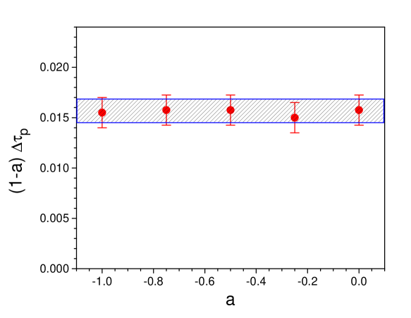
Figure 1: Shifts of the peaks $\Delta\tau_{p}(a,Q=91\mbox{ GeV})$ of the distributions $\left(1/\sigma_{\mbox{\tiny tot}}\right)d\sigma/d\tau_{a}$ between NLL partonic resummed predictions and hadronic cross sections computed using PYTHIA with string fragmentation. The result is multiplied by $(1-a)$. The error bars are estimated from the uncertainty of the NLL resummed calculation and the output of PYTHIA. The shaded band is the shift of the peak for the thrust determined in [14] between resummed predictions and experimental data.

5.2 Shape functions

Now let us turn to the full shape functions. We will test the scaling directly in moment space, where a parameterization in terms of the coefficients $\lambda_{n}$ of Eq. (28) is most straightforward. Using Eq. (27), we have

$$\tilde{f}_{a,{\rm NP}}\left(\frac{\nu}{Q},\kappa\right)={\tilde{R}(\nu,Q,a)\over\tilde{R}_{{\rm PT}}(\nu,Q,\kappa,a)}+{\cal O}\left({1\over Q^{1-a}}\right)\,.$$ (36)

This gives moment space expressions for the shape functions directly, given experimental or other input for $\tilde{R}(\nu,Q,a)$ in the numerator and resummed perturbation theory (in our case to NLL) for $\tilde{R}_{{\rm PT}}(\nu,Q,\kappa,a)$ in the denominator. As above, we use the output of PYTHIA for the numerator. For the denominator, we use the method described above in Sec. 3.3.

The results are shown in Fig. 2 at $Q=91$ GeV and in Fig. 3 at $Q=35$ GeV. We begin by computing the shape functions for $a=0,\,-0.25,\,-0.5$ at $Q=91$ GeV and $Q=35$ GeV directly from Eq. (36). These are the solid curves in the figures. The dotted curves show the predictions found by simply scaling the $a=0$ curve in each case according to Eq. (29), or equivalently

$$\tilde{f}_{a,{\rm NP}}\left(\frac{\nu}{Q},\kappa\right)=\left[\,\tilde{f}_{0,{\rm NP}}\left(\frac{\nu}{Q},\kappa\right)\,\right]^{1\over 1-a}\,.$$ (37)

The perturbative radiator defined in Eq. (26), and thus the ratio in (37), as plotted in Figs. 2 and 3, are fairly dependent on the value of the cutoff $\kappa$. This dependence compensates of course between perturbative and nonperturbative contributions to the full radiator (27).

As in the case of the shifts, we see that within the range of parameter $a$ considered, the scaling works well. It is worth pointing out that a similar scaling fails by a relatively large amount for the perturbative cross section itself. We have restricted ourselves to a minimum value of $a=-0.5$ to keep an acceptable numerical accuracy.

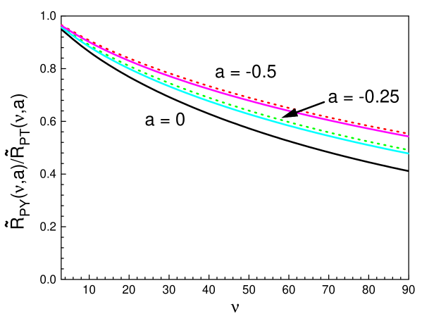
Figure 2: The ratios, Eq. (36), between the output of PYTHIA and the NLL resummed predictions at $a=0,-1/4,-1/2$ at c.m. energy $Q=91$ GeV. The solid lines are the directly computed ratios, the dotted lines is the scaled $a=0$ curve, according to Eq. (37).

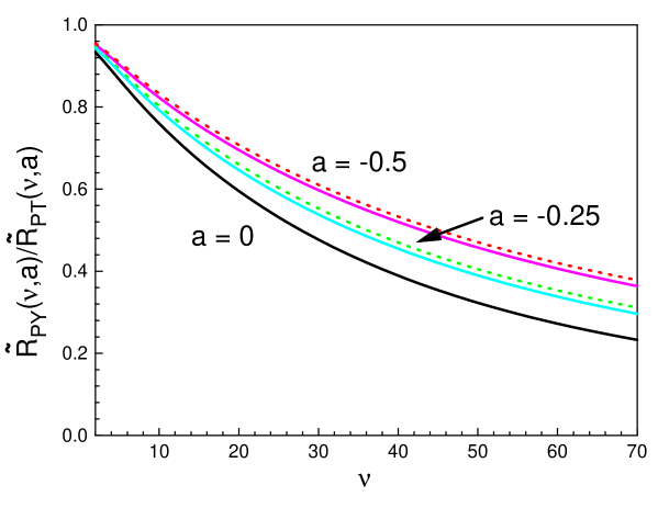
Figure 3: The ratios, Eq. (36), between the output of PYTHIA and the NLL resummed predictions at $a=0,-1/4,-1/2$ at c.m. energy $Q=35$ GeV, solid and dotted lines as in Fig. 2.

We note that the logarithms of the curves in both figures depend fairly linearly on $\nu$ for relatively small $\nu$, indicating that in this range the linear, $\nu/Q$ term dominates. This is consistent with the result above for the shifts, which is based only on the $\nu/Q$ correction. To fit the curves at larger $\nu$, however, higher powers in $\nu/Q$ are necessary. While we have not attempted a fit of the $a=0$ case (thrust) at different energies our reasoning is consistent with any determination of the coefficients $\lambda_{n}(\kappa)$ in Eq. (28) [23, 25, 26].

We emphasize that the agreement of our scaling rule with PYTHIA may only mean that the output of PYTHIA shares some of the properties that go into the derivation of the rule.

5.3 Scaling violations

In the light of the relation between the scaling rule and boost invariance, Sec. 4.2, we can understand why PYTHIA respects the rule over a moderate range of parameter $a$. It is natural to think of jet fragmentation as dynamically boost-invariant along the jet axis, while boost invariance need not be respected for coherent interjet radiation, which depends on the relative directions of the jets. For moderate values of $a$, the shape functions may follow the scaling in our numerical tests because in PYTHIA the corresponding event weights are dominated by particles created from boost-invariant dynamics, and for which correlations between the jet hemispheres (for example, due to decays into opposite hemispheres) are negligible.

Beyond NLL, however, the general resummation for the two-jet event shapes of Eq. (4) involves coherent interjet radiation [18], which we expect to produce correlations between the jet hemispheres. The neglect of such correlations is related to the “inclusive” approximation discussed in Ref. [25], in which the effect on the weight function from off-shell gluons that split into particles that move into different hemispheres is suppressed.

More generally, suppose that the correlation between energy flow is enhanced relative to NLL perturbation theory for “short-range” rapidity intervals, less than some constant $\Delta\eta_{0}$. Then, because of correlations between radiation in different hemispheres, the scaling implied by Eq. (32) can hold only when the rapidity range for each term on the right-hand side is much larger than the constant, $[n(1-a)]^{-1}\gg\Delta\eta_{0}$. For any $\Delta\eta_{0}$, this condition is violated for $n$ large enough. Thus, as $(1-a)$ increases, the scaling is violated, first by high powers of $\nu/Q$, and eventually by lower powers. Only to the extent that enhanced short-range correlations are fully negligible can we expect that the scaling holds for the full shape function. Pushing our analysis to larger values of $(1-a)$ should eventually uncover correlations between hemispheres, even in PYTHIA, perhaps associated with the string breaking picture of hadronization. In general, we would expect physical moments to decrease less rapidly than $(1-a)^{-1}$ in the presence of positive correlations between radiation in different hemispheres [24].

The extension of our analysis to multijet events [28] should be relatively straightforward. In this case, as in the two-jet limit of $\rm e^{+}e^{-}$ annihilation, it is necessary to determine each jet axis by a thrust-like condition, which is relatively insensitive to recoil effects [17, 18], to insure resummation at NLL. Such cross sections still factorize perturbatively, but now into a function involving coherent interjet radiation as well as jet functions, even at NLL. The jet functions, but not the soft function, should obey a scaling relation like Eq. (29). Tests of this scaling for multi-jet shape functions could be an indirect way to estimate the significance of coherence effects for interjet radiation. Extensions to deep-inelastic scattering [19] and hadronic scattering [28] may also be possible.

6 Conclusions

We have derived a scaling property that relates nonperturbative shape functions within the class of event shapes, including the thrust, introduced in [18]. We have seen that the resulting predictions match the output of the event generator PYTHIA over a range of the relevant parameter that defines the event shape. This analysis is based on the NLL resummed cross section for these event shapes, which neglects correlations between hemispheres. The comparison of these predictions to actual data should shed light on universality properties of nonperturbative corrections, and their relationship to determinations of $\alpha_{s}$. We hope that this comparison is still possible for archived data from LEP.

We have argued that the scaling rule derived from the NLL cross section is more generally dependent on the boost invariance of strong coupling dynamics. In general, the scaling must also fail at some level due to correlations between hemispheres, associated for example with decays [24, 36]. We might expect such effects to become more important for $a\ll-1$, since the corresponding weight functions are sensitive primarily to radiation near the boundary between the hemispheres. In any case, we hope that the example studied above shows that event shapes can be designed to probe specific aspects of nonperturbative QCD dynamics.

Appendix A Explicit Expressions for the Cross Section in Transform Space

For the evaluation of the integrals in Eq. (9) we use the running coupling at renormalization scale $\mu$ in terms of the coupling $\alpha$ evaluated at $Q/2$, expanded for use at NLL accuracy,

$$\alpha \equiv \alpha_{s}\left(\frac{Q}{2}\right)$$ (38)

$$\alpha_{s}(\mu) = \frac{\alpha}{1+\frac{\beta_{0}}{2\pi}\alpha\ln\frac{2\mu}{Q}}\left[1-\frac{\beta_{1}}{4\pi\beta_{0}}\frac{\alpha}{1+\frac{\beta_{0}}{2\pi}\alpha\ln\frac{2\mu}{Q}}\ln\left(1+\frac{\beta_{0}}{2\pi}\alpha\ln\frac{2\mu}{Q}\right)+\dots\right],$$

where the coefficients $\beta_{0}$ and $\beta_{1}$ are given by

$$\beta_{0} = \frac{11}{3}C_{A}-\frac{4}{3}T_{F}N_{f},$$ (40)

$$\beta_{1} = \frac{34}{3}C_{A}^{2}-\frac{20}{3}C_{A}T_{F}N_{f}-4C_{F}T_{F}N_{f}.$$ (41)

The term with $\beta_{1}$ is only necessary for the integral containing $A^{(1)}$ at NLL.

Inserting the expansion of (38) into Eq. (9), the integrals are done to NLL accuracy in terms of elementary functions by using the replacement $\left(\exp[-y]-1\right)\rightarrow-\theta\left(y-{\rm e}^{-\gamma_{E}}\right)$, which is accurate to NLL. Here $\gamma_{E}$ is the Euler constant. The result of this procedure is,

$${1\over\sigma_{\rm tot}}\tilde{\sigma}\left(\nu,Q,a\right) \equiv \left[\,{\mathcal{J}}(\nu,Q,a)\right]^{2}$$ (42)

$$= \exp\Bigg{\{}2\,\ln(\nu)\,g_{1}\left(\frac{\beta_{0}}{2\pi}\frac{\alpha_{s}(\mu)}{2-a}\ln\nu,a\right)$$

$$\qquad+\,2\,\left(\frac{\beta_{0}}{2\pi}\right)^{2}\frac{\alpha_{s}^{2}(\mu)}{2-a}\ln^{2}\nu\,\ln\left(\frac{2\mu}{Q}\right)g_{1}^{\prime}\left(\frac{\beta_{0}}{2\pi}\frac{\alpha_{s}(\mu)}{2-a}\ln\nu,a\right)$$

$$\qquad+\,2\,g_{2}\left(\frac{\beta_{0}}{2\pi}\frac{\alpha_{s}(\mu)}{2-a}\ln\nu,a\right)+{\mathcal{O}}\left(\alpha_{s}^{n}\ln^{n-1}\nu\right)\Bigg{\}},$$

where the functions $g_{1}$ and $g_{2}$ and $g^{\prime}_{1}$ that resum leading and next-to-leading logarithms, respectively, are given by

$$g_{1}(x,a) = -\frac{4}{\beta_{0}}\frac{1}{1-a}\frac{1}{x}A^{(1)}\Bigg{[}\left(\frac{1}{2-a}-x\right)\ln(1-(2-a)x)-\,(1-x)\ln(1-x)\Bigg{]}$$

$$g_{2}(x,a) = \frac{2}{\beta_{0}}B^{(1)}\ln(1-x)-\frac{8}{\beta_{0}^{2}}\frac{1}{1-a}A^{(2)}\left[(2-a)\ln(1-x)-\ln(1-(2-a)x)\right]$$ (44)

$$-\,\frac{4}{\beta_{0}}\gamma_{E}\frac{1}{1-a}A^{(1)}\left[\ln(1-x)-\ln(1-(2-a)x)\right]$$

$$+\,\frac{4}{\beta_{0}}\ln 2\frac{1}{1-a}\,A^{(1)}\left[(2-a)\ln(1-x)-\ln(1-(2-a)x)\right]$$

$$-\frac{\beta_{1}}{\beta_{0}^{3}}\frac{1}{1-a}A^{(1)}\left[2\ln(1-(2-a)x)-2(2-a)\ln(1-x)\right.$$

$$\qquad\qquad\qquad+\left.\,\ln^{2}(1-(2-a)x)-(2-a)\ln^{2}(1-x)\right]$$

$$g_{1}^{\prime}\left(x,a\right) = \frac{\partial}{\partial x}g_{1}(x,a).$$ (45)

In Eq. (42) the scale $\mu$ should be chosen of the order of the hard scale to avoid further large logarithms, and we choose $\mu=Q$. Setting $\mu=Q$ as in [16] cancels the term proportional to $\ln 2$ in Eq. (44), and we reproduce for $a=0$ the form of [16].

Finally, for sake of completeness, we list the coefficients $G_{ij}$ that occur in the expansion in terms of $\alpha_{s}$ of the logarithm of the resummed radiator, Eq. (22),

$$G_{11}(a) = \frac{3}{2-a}C_{F},$$ (46)

$$G_{12}(a) = -\frac{2}{2-a}C_{F},$$ (47)

$$G_{22}(a) = -\frac{1}{(2-a)^{2}}\frac{1}{36}C_{F}\left[48\pi^{2}C_{F}+\left(169-134\,a-6\,(2-a)\pi^{2}\right)C_{A}\right.$$ (48)

$$\qquad\qquad\qquad\qquad\left.-2\,(11-10\,a)N_{f}\right],$$

$$G_{23}(a) = -\frac{3-a}{(2-a)^{2}}\frac{1}{9}C_{F}\left(11C_{A}-2N_{f}\right).$$ (49)

For $a=0$, the $G_{ij}$s again reduce to those listed in [16].

References

- [1] E. Farhi, Phys. Rev. Lett. 39, 1587 (1977).
-
[2]
H. Georgi and M. Machacek,
Phys. Rev. Lett. 39, 1237 (1977);
G. Parisi, Phys. Lett. B 74, 65 (1978);
J. F. Donoghue, F. E. Low and S. Y. Pi, Phys. Rev. D 20, 2759 (1979);
G. C. Fox and S. Wolfram, Nucl. Phys. B 149, 413 (1979) [Erratum-ibid. B 157, 543 (1979)]. - [3] S. Catani, G. Turnock and B. R. Webber, Phys. Lett. B 295, 269 (1992).
- [4] T. Chandramohan and L. Clavelli, Nucl. Phys. B 184, 365 (1981).
-
[5]
C. L. Basham, L. S. Brown, S. D. Ellis and S. T. Love,
Phys. Rev. D 17, 2298 (1978);
N. A. Sveshnikov and F. V. Tkachov, Phys. Lett. B 382, 403 (1996) [hep-ph/9512370];
F. V. Tkachov, Int. J. Mod. Phys. A 12, 5411 (1997) [hep-ph/9601308];
G. P. Korchemsky, G. Oderda and G. Sterman, in 5th International Workshop on Deep Inelastic Scattering and QCD (DIS 97), AIP Conference Proceedings 407, ed. J. Repond, D. Krakauer (American Institute of Physics, Woodbury, NY 1978), p. 988 [hep-ph/9708346];
C. F. Berger et al., in Proc. of the APS/DPF/DPB Summer Study on the Future of Particle Physics (Snowmass 2001) ed. N. Graf, eConf C010630, P512 (2001) [hep-ph/0202207]. -
[6]
H. Contopanagos and G. Sterman, Nucl. Phys. B 419, 77 (1994)
[hep-ph/9310313];
B. R. Webber, Phys. Lett. B 339, 148 (1994) [hep-ph/9408222];
Y. L. Dokshitzer and B. R. Webber, Phys. Lett. B 352, 451 (1995) [hep-ph/9504219];
R. Akhoury and V. I. Zakharov, Nucl. Phys. B 465, 295 (1996) [hep-ph/9507253];
M. Beneke, V. M. Braun and L. Magnea, Nucl. Phys. B 497, 297 (1997) [hep-ph/9701309];
M. Beneke and V.M. Braun, in the Boris Ioffe Festschrift, At the Frontier of Particle Physics / Handbook of QCD, ed. M. Shifman (World Scientific, Singapore, 2001), vol. 3, p. 1719 [hep-ph/0010208]. - [7] A. V. Manohar and M. B. Wise, Phys. Lett. B 344, 407 (1995) [hep-ph/9406392].
-
[8]
G. P. Korchemsky and G. Sterman, Nucl. Phys. B
437, 415 (1995)
[hep-ph/9411211];
G. P. Korchemsky and G. Sterman, in Moriond 1995: Hadronic:0383-392 [hep-ph/9505391]. - [9] Y. L. Dokshitzer and B. R. Webber, Phys. Lett. B 404, 321 (1997) [hep-ph/9704298].
-
[10]
Y. L. Dokshitzer, G. Marchesini and B. R. Webber,
Nucl. Phys. B 469, 93 (1996)
[hep-ph/9512336];
Y. L. Dokshitzer, A. Lucenti, G. Marchesini and G. P. Salam, Nucl. Phys. B 511, 396 (1998) [Erratum-ibid. B 593, 729 (2001)] [hep-ph/9707532];
Y. L. Dokshitzer, A. Lucenti, G. Marchesini and G. P. Salam, JHEP 9805, 003 (1998) [hep-ph/9802381];
Y. L. Dokshitzer, G. Marchesini and G. P. Salam, Eur. Phys. J. direct C 1, 3 (1999) [hep-ph/9812487];
Y. L. Dokshitzer, G. Marchesini and B. R. Webber, JHEP 9907, 012 (1999) [hep-ph/9905339];
M. Dasgupta, L. Magnea and G. Smye, JHEP 9911, 025 (1999) [hep-ph/9911316]. -
[11]
A. H. Mueller,
Phys. Lett. B 308, 355 (1993);
M. Dasgupta and B. R. Webber, Phys. Lett. B 382, 273 (1996) [hep-ph/9604388];
M. Dasgupta and B. R. Webber, Eur. Phys. J. C 1, 539 (1998) [hep-ph/9704297];
M. Dasgupta and B. R. Webber, JHEP 9810, 001 (1998) [hep-ph/9809247]. - [12] C. Adloff et al. [H1 Collaboration], Phys. Lett. B 406, 256 (1997) [hep-ex/9706002].
-
[13]
S. Bethke,
J. Phys. G 26, R27 (2000)
[hep-ex/0004021];
S. J. Burby and C. J. Maxwell, Nucl. Phys. B 609, 193 (2001) [hep-ph/0011203];
G. Dissertori, Measurements of alpha(s) from event shapes and the four-jet rate, [hep-ex/0209070]. - [14] P. A. Movilla Fernandez, S. Bethke, O. Biebel and S. Kluth, Eur. Phys. J. C 22, 1 (2001) [hep-ex/0105059].
- [15] S. Catani, G. Turnock, B. R. Webber and L. Trentadue, Phys. Lett. B 263, 491 (1991).
- [16] S. Catani, L. Trentadue, G. Turnock and B. R. Webber, Nucl. Phys. B 407, 3 (1993).
- [17] Y. L. Dokshitzer, A. Lucenti, G. Marchesini and G. P. Salam, JHEP 9801, 011 (1998) [hep-ph/9801324].
-
[18]
C. F. Berger, T. Kúcs and G. Sterman, Interjet energy flow
/ event shape correlations, hep-ph/0212343;
C. F. Berger, T. Kúcs and G. Sterman, Phys. Rev. D 68, 014012 (2003) [hep-ph/0303051]. -
[19]
M. Dasgupta and G. P. Salam,
JHEP 0208, 032 (2002)
[hep-ph/0208073];
M. Dasgupta and G. P. Salam, Eur. Phys. J. C 24, 213 (2002) [hep-ph/0110213]. - [20] M. Dasgupta and G. P. Salam, Phys. Lett. B 512, 323 (2001) [hep-ph/0104277].
- [21] G. P. Korchemsky and G. Sterman, Nucl. Phys. B 555, 335 (1999) [hep-ph/9902341].
- [22] G. P. Korchemsky, Shape functions and power corrections to the event shapes, in Minneapolis 1998, Continuous advances in QCD, 179 (1998) [hep-ph/9806537].
- [23] G. P. Korchemsky and S. Tafat, JHEP 0010, 010 (2000) [hep-ph/0007005].
- [24] A. V. Belitsky, G. P. Korchemsky and G. Sterman, Phys. Lett. B 515, 297 (2001) [hep-ph/0106308].
- [25] E. Gardi and J. Rathsman, Nucl. Phys. B 609, 123 (2001) [hep-ph/0103217].
- [26] E. Gardi and J. Rathsman, Nucl. Phys. B 638, 243 (2002) [hep-ph/0201019].
- [27] E. Gardi and L. Magnea, The C parameter distribution in annihilation, hep-ph/0306094.
-
[28]
A. Banfi, Y. L. Dokshitzer, G. Marchesini and G. Zanderighi,
JHEP 0103, 007 (2001)
[hep-ph/0101205];
A. Banfi, G.P. Salam and G. Zanderighi, Generalized resummation of QCD final-state observables, hep-ph/0304148. - [29] T. Sjostrand, P. Eden, C. Friberg, L. Lonnblad, G. Miu, S. Mrenna and E. Norrbin, Comput. Phys. Commun. 135, 238 (2001) [hep-ph/0010017].
- [30] G. P. Salam and D. Wicke, JHEP 0105, 061 (2001) [hep-ph/0102343].
- [31] G. Sterman, Approaching the final state in perturbative QCD, hep-ph/0301243.
- [32] S. Catani and M. H. Seymour, Phys. Lett. B 378, 287 (1996) [hep-ph/9602277].
- [33] N. Kidonakis, G. Oderda and G. Sterman, Nucl. Phys. B 531, 365 (1998) [hep-ph/9803241].
-
[34]
G. Sterman,
in AIP Conference Proceedings Tallahassee, Perturbative Quantum Chromodynamics,
eds. D. W. Duke, J. F. Owens, New York, 1981;
J. G. Gatheral, Phys. Lett. B 133, 90 (1983);
J. Frenkel and J. C. Taylor, Nucl. Phys. B 246, 231 (1984);
G. P. Korchemsky and A. V. Radyushkin, Phys. Lett. B 171, 459 (1986);
C. F. Berger, Phys. Rev. D 66, 116002 (2002) [hep-ph/0209107]. - [35] C. F. Berger, Soft gluon exponentiation and resummation, Ph.D. Thesis, SUNY at Stony Brook, May 2003, hep-ph/0305076.
- [36] P. Nason and M. H. Seymour, Nucl. Phys. B 454, 291 (1995) [hep-ph/9506317].
- [37] T. Sjostrand, L. Lonnblad and S. Mrenna, PYTHIA 6.2: Physics and manual, [hep-ph/0108264].
-
[38]
B. Andersson, G. Gustafson, G. Ingelman and T. Sjostrand, Phys. Rept. 97, 31 (1983);
B. Andersson, The Lund Model, Cambridge Monogr. Part. Phys. Nucl. Phys. Cosmol. 7, 1 (1997).