Abstract

We study the Higgs-boson decays $h^{0}\to b\bar{b}$, $h^{0}\to\gamma\gamma$ and $h^{0}\to\gamma Z$ within the framework of the Two Higgs Doublet Model (THDM) in the context of the decoupling regime, together with tree level unitarity constraints. We show that when the light CP-even Higgs boson of the THDM mimics the Standard-Model Higgs boson, not only the one-loop effects to $h^{0}\to\{\gamma\gamma,\gamma Z\}$ but also the one-loop contribution to $h^{0}\to b\bar{b}$ can be used to distinguish between THDM and SM. The size of the quantum effects in $h^{0}\to b\bar{b}$ are of the same order as in $h^{0}\to\{\gamma\gamma,\gamma Z\}$ and can reach 25% in both cases.

PACS: 14.80.Cp, 14.80.Bn, 13.90.+i, 12.60.Fr
Keywords: THDM, neutral Higgs boson, decoupling limit, unitarity.

1 Introduction

The discovery of a Higgs boson is one of the major goals of present and future searches in particle physics. Global electroweak fits within the Standard Model (SM) yield an upper bound on the Higgs-boson mass of $M_{H}<211$ GeV at $95\%$ confidence level (CL) [1]. Together with the direct-search limit from the LEP experiments [2] of $M_{H}>114.4$ GeV, the Higgs boson seems “just around the corner”.

The still hypothetical Higgs sector of the SM can be enlarged and some simple extensions such as the Two Higgs Doublet Model (THDM) versions [3] are intensively studied. Such extensions add new phenomena, like the charged Higgs-boson sector, and satisfies the relevant constraint $\rho\approx 1$ up to finite radiative corrections. Actually, there are two versions of the THDM, type I and type II, differing in some Higgs couplings to fermions, but in both types and after electroweak symmetry breaking, the Higgs spectrum is the same: two charged Higgs particles $H^{\pm}$, two CP-even $H^{0}$, $h^{0}$ and one CP–odd $A^{0}$. Aside the charged Higgs sector, the neutral sector of the THDM is noticeably different from the SM single-Higgs sector. Whereas the discovery of a charged scalar Higgs boson would attest definitively that the Standard Model is overcome, more refined investigations would be necessary in case of a neutral Higgs particle, in the SM and beyond [4].

In order to establish the Higgs mechanism for the electroweak symmetry breaking, we need to measure the Higgs couplings to fermions and to gauge bosons as well as the self-interaction of Higgs bosons. Such measurements, if precise enough, can be helpful in discriminating between the models through their sensitivity to quantum-correction effects, in particular in specific cases like the decoupling limit. For a Linear Collider, it has been shown [5] that the Higgs-boson couplings to third-generation fermions and gauge bosons can be measured with high precision of the order 1–3%.

The decoupling theorem [6] states, in brief, that, if we have a theory with light and heavy particles, under certain conditions, the effects of heavy particles only appear in the low-energy theory through renormalization of couplings and masses of the effective theory or through corrections proportional to a negative power of the heavy masses. The decoupling theorem is not universal and suffers from some known exceptions [7]. To be sure that the theorem holds, the low-energy theory has to be renormalizable, and it should have neither spontaneous symmetry breaking nor chiral fermions, which does not apply to the MSSM and the THDM. A formal and general proof of decoupling of the non-standard MSSM particles from the low-energy electroweak gauge-boson physics has been given in [8]. Conversely, concerning Higgs physics, it is known that the SUSY one-loop corrections do not decouple, in general, in the limit of a heavy supersymmetric spectrum [9, 10, 11, 12, 13, 14, 15].

Furthermore, it is not yet rigorously proven that this decoupling theorem applies in the case of the THDM [16]. But one can be less ambitious and consider a weaker version for the decoupling limit [17], where all the scalar masses with one exception formally become infinite. For the case of the THDM, this limit designs the CP-even $h^{0}$ as the light scalar particle while the other Higgs particles, the CP-even $H^{0}$, the CP-odd $A^{0}$, and the charged Higgs boson $H^{\pm}$ are extremely heavy and mass-degenerate. In using pure algebraic arguments at the tree level, and more sophisticated ones at the loop level, one can derive the main consequences: in the decoupling limit, $\cos(\beta-\alpha)\to 0$, the CP-even $h^{0}$ of the THDM and the SM Higgs $H$ have quite similar tree level couplings to gauge bosons and fermions as well [16]. Here $\alpha$ is the mixing angle in the CP-even sector and $\tan\beta=v_{1}/v_{2}$, the ratio of the two vacuum expectation values[3]. Since the scalar sector of the MSSM is a particular case of THDM, the various decoupling scenarios also take place in the MSSM and give similar consequences as in the THDM.

Obviously, the decoupling limit does not rigorously apply to a more realistic world where the particles masses are in a finite range. Actually, one may consider a less rigorous scenario, labeled as the decoupling regime [16, 17, 18], where we only require that the heavy Higgs particles have masses much larger than the $Z$ boson mass. However, such a scenario with large masses has to agree with the unitarity of the $S$-matrix. The unitarity constraint puts in turn bounds on the amplitude of partial waves [19], which give finally constraints on the values of the coupling constants. The problem in models with symmetry breaking is that couplings and masses are not independent; hence, unitarity of the $S$-matrix implies upper bounds on masses in the SM as well as in the THDM.

Since perturbative expansion is used, it is impossible to find the exact bounds; instead, one can derive tree-level unitarity bounds or loop-improved unitarity bounds. In this study, we will use unitarity bounds coming from a tree-level analysis [20]. This tree level analysis is derived with the help of the equivalence theorem [21], which itself is a high-energy approximation where it is assumed that the energy scale is much larger than the $Z^{0}$ and $W^{\pm}$ gauge-boson masses. We will consider here this “high-energy” hypothesis that both the equivalence theorem and the decoupling regime are well settled, but in such a way that the unitarity constraint is also fulfilled. Our purpose is to investigate the quantum effects in the decays of the light CP-even Higgs boson $h^{0}$, especially looking for sizeable differences with respect to the SM in the decoupling regime.

Several studies have been carried out looking for non-decoupling effects in Higgs-boson decays and Higgs self-interactions. Large loop effects in $h^{0}\to\gamma\gamma$ and $h^{0}\to\gamma Z$ have been pointed out for both the MSSM [12] and the THDM [22]. The one-loop SUSY-QCD effects in $h^{0}\to b\bar{b}$ were addressed in [13] and their decoupling properties are well discussed and understood. The loop contribution to the triple $h^{0}$ self-coupling has been investigated in the MSSM [14] as well as in the THDM [15], revealing non-decoupling effects which, however, in the MSSM case disappear when the self-coupling is expressed in terms of the $h^{0}$ mass [14].

The present study assumes the following chronology and scenario: the SM model is not ruled out by any experiment, no SUSY evidence, no charged Higgs and no CP-odd Higgs signal, a light CP-even Higgs is detected and its properties are rather close to the SM Higgs. A very natural question emerges: what kind of Higgs we got? It seems difficult to disentangle the Higgs particle of the basic SM from other Higgs bosons involved in extended models like the THDM or MSSM. We will focus on the perhaps most difficult scenario, where all the Higgs particles of the THDM, except the lightest CP-even Higgs, are heavy to escape detection at the first stage of next generation colliders.

In this paper we investigate three decay modes of the CP-even neutral Higgs boson $h^{0}$ (THDM) or $H$ (SM): the decay into a pair of photons, the decay into a photon in association with a $Z$ boson, and the decay into a $b\bar{b}$ quark pair. The decays into the gauge-boson pairs are loop-mediated processes since the photon does not couple to neutral particles. In contrast, the decay into a fermion pair already exists at the tree level because of the Higgs–$b$ Yukawa interaction. For the specific scenario where only a single light Higgs particle exists with tree-level coupling constants as in the SM, the coupling structure of the virtual non-standard heavy particles in the quantum contributions to the bosonic decay rates yield sizeable differences to the SM decay rates. Simultaneously, these quantum corrections also influence the fermionic decay rates and thus make them differ significantly from the SM result as well.

The paper is organized as follows. In section 2 we address the Higgs-boson decay channels under study and outline the calculation of the one-loop contribution to the $h^{0}\to b\bar{b}$ partial width, giving details about the renormalization scheme used. Section 3 is devoted to the presentation and discussion of our numerical results.

2 Decays of the ${\bf\boldmath{h^{0}}}$ boson in the THDM

In this section, we first discuss the one-loop contributions to $h^{0}\to\gamma\gamma$ and $h^{0}\to\gamma Z$, which have been known already for a while [3]. Then, we present in more details the one-loop contribution to $h^{0}\to b\bar{b}$ as well as details of the renormalization scheme used.

We first start with the decay channels $h^{0}\to\gamma\gamma$ and $h^{0}\to\gamma Z$, which are loop-induced, the only pure THDM contribution comes from charged Higgs loops, which may lead to non-decoupling effects. In the decoupling regime, with $\alpha\rightarrow\beta-\pi/2$, the charged Higgs contribution enters at the one-loop level through the following coupling,

$$g[h^{0}H^{+}H^{-}] = -\frac{g}{2M_{W}}\{M_{h^{0}}^{2}+2(M_{H^{\pm}}^{2}-\lambda_{5}v^{2})\}$$ (1)

where $v^{2}=v_{1}^{2}+v_{2}^{2}=(2\sqrt{2}G_{F})^{-1}$ . To derive this coupling we have used the CP conserving scalar potential of ref. [3], where the parameter $\lambda_{5}$ breaks softly the discrete symmetry $\Phi_{1}\to-\Phi_{1}$. The decay rates of $h^{0}\to\gamma\gamma$ and $h^{0}\to\gamma Z$ are taken from ref. [3]. From the form of the coupling in eq. (1), one can see that the quadratic term $M_{H^{\pm}}^{2}$ can be compensated by $\lambda_{5}v^{2}$. With charged Higgs-boson masses much larger than the electroweak scale ($M_{H^{\pm}}>v$), such cancellations take place only for large values of $\lambda_{5}$ [17]. For fixed $M_{h^{0}}$ and $M_{H^{\pm}}$, the charged Higgs contribution, entering through eq. (1), vanishes for the critical choice of $\lambda_{5}=\lambda_{5}^{0}$, where

$$\lambda_{5}^{0}=\frac{1}{2v^{2}}\{M_{h^{0}}^{2}+2M_{H^{\pm}}^{2}\}.$$ (2)

For the Higgs decay $h^{0}\to b\bar{b}$, we evaluate the partial width $\Gamma({h^{0}\to b\bar{b}})$ at the one-loop level, in both the SM and the THDM, using the SM width as a reference. The model-independent contributions, QCD and QED corrections, are not included. For $\Gamma({H\to b\bar{b}})$ in the SM, we have performed the calculation in the on-shell scheme [24], in analogy to the work presented in [23]. Practical computations were done with the help of the packages FeynArts, FormCalc [25], and with LoopTools and FF for numerical evaluations [26]. The THDM is nowadays available in the package FeynArts.

At one-loop order the amplitude can be written as follows,

$${\cal M}_{1}=-\frac{igm_{b}}{2M_{W}c_{\beta}}\,\sqrt{Z_{h^{0}}}\left[s_{\alpha}\,(1+\Delta{\cal M}_{1})+s_{\alpha}\,\Delta{\cal M}_{12}\right]$$ (3)

with $s_{\alpha}=\sin\alpha\,,c_{\beta}=\cos\beta$, and

$$\Delta{\cal M}_{1} = V_{1}^{h^{0}b\bar{b}}+\delta(h^{0}b\bar{b})\,\,\,,\,\,\,\Delta{\cal M}_{12}=\frac{\Sigma_{hH}(M_{h^{0}}^{2})}{M_{h^{0}}^{2}-M_{H^{0}}^{2}}-\delta\alpha\,,$$

$$Z_{h^{0}} = \left[1+\widehat{\Sigma}_{h^{0}}^{\prime}(M_{h^{0}}^{2})\right]^{-1}\,.$$ (4)

These expressions contain the vertex corrections $V_{1}^{h^{0}b\bar{b}}$ with the corresponding vertex counterterm $\delta(h^{0}b\bar{b})$, the non-diagonal $h^{0}$–$H^{0}$ self-energy $\Sigma_{hH}$ with the counterterm $\delta\alpha$ for the mixing angle $\alpha$, and the wave-function renormalization with the $h^{0}$ field-renormalization constant $Z_{h^{0}}$ derived from the renormalized self-energy of the $h^{0}$.

In the general THDM, the mixing angle $\alpha$ is an independent parameter and can hence be renormalized in a way independent of all the other renormalization conditions. A simple and natural condition is to require that $\delta\alpha$ absorbs the $h^{0}$–$H^{0}$ transition in the non-diagonal part $\Delta{\cal M}_{12}$ of the decay amplitude (3). The angle $\alpha$ is hence the CP-even Higgs-boson mixing angle also at the one-loop level, and the decay amplitude ${\cal M}_{1}$ simplifies to the $\Delta{\cal M}_{1}$ term only. The Higgs-boson decay width is then given by the expression

$$\Gamma_{1}(h^{0}\to b\bar{b})=\frac{N_{C}G_{F}m_{b}^{2}}{4\sqrt{2}\pi}\frac{s_{\alpha}^{2}}{c_{\beta}^{2}}\,M_{h^{0}}\,Z_{h^{0}}\,[1+2\Re(\Delta{\cal M}_{1})]\,.$$ (5)

The central part of the computation is thus the determination of $\Delta{\cal M}_{1}$. The generic THDM contributions to $\Delta{\cal M}_{1}$ are depicted in Fig. 1, involving vertex-correction and counterterm diagrams. A quick inspection shows that there are pure THDM contributions not present in the SM case: diagram $d_{1}$ with $S=H^{0},A^{0},H^{\pm}$, diagram $d_{2}$ with $(S_{1},S_{2})=(H^{0},H^{0})$, $(A^{0},A^{0})$, $(H^{\pm},H^{\pm})$ and $(H^{\pm},G^{\pm})$, and lastly diagrams $d_{4,5}$ with $S=A^{0},H^{\pm}$. In the decoupling limit, diagrams $d_{4,5}$ and diagram $d_{2}$ with $(S_{1},S_{2})$=$(H^{\pm},G^{\pm})$ vanish. As a consequence, large effects in $h^{0}\to b\bar{b}$ may arise from diagrams $d_{1}$ and $d_{2}$. Thereby, $d_{2}$ formally has non-decoupling behaviour, yielding a non-zero value in the mathematical limit of heavy non-standard particles.

We refrain here from giving analytical expressions for the vertex corrections; the MSSM formulae given in [27] can be adapted to the THDM case replacing the MSSM couplings by the THDM ones [17, 28].

Figure 1: Generic one-loop THDM Feynman diagrams contributing to $\Gamma({h^{0}\to b\bar{b}})$.

We will use the on-shell scheme based on [29] for determination of the counterterms, with the exception that the field renormalization constants for the two Higgs doublets are determined in the ${\overline{\rm MS}}$ scheme, yielding $Z_{\Phi_{i}}=1+\delta Z_{\Phi_{i}}^{\overline{\rm MS}}$,

$$\delta Z_{\Phi_{1}}^{\overline{\rm MS}} = \frac{-g^{2}\Delta}{32\pi^{2}m_{W}^{2}}\{\frac{1}{c_{\beta}^{2}}(m_{e}^{2}+m_{\mu}^{2}+m_{\tau}^{2}+(m_{b}^{2}+m_{d}^{2}+m_{s}^{2})N_{C})\}+\frac{\Delta}{2(4\pi)^{2}}(3g^{2}+g^{\prime 2})\,,$$

$$\delta Z_{\Phi_{2}}^{\overline{\rm MS}} = \frac{-g^{2}\Delta}{32\pi^{2}m_{W}^{2}}\{\frac{N_{C}}{s_{\beta}^{2}}(m_{c}^{2}+m_{t}^{2}+m_{u}^{2})\}+\frac{\Delta}{2(4\pi)^{2}}(3g^{2}+g^{\prime 2})\,,$$ (6)

with $\Delta=2/(4-D)-\gamma+{\rm log}4\pi$ from dimensional regularization and the color factor $N_{C}$. Accordingly, the $h^{0}$ field-renormalization constant is a linear combination of (2), which determines the derivative of the renormalized self-energy in (2) to be

$$\widehat{\Sigma}_{h^{0}}^{\prime}(M_{h^{0}}^{2})=\Sigma_{h^{0}}^{\prime}(M_{h^{0}}^{2})+(\delta Z_{\Phi_{1}}^{\overline{MS}}\sin^{2}\alpha+\delta Z_{\Phi_{2}}^{\overline{MS}}\cos^{2}\alpha)\,,$$ (7)

in terms of the unrenormalized self-energy ${\Sigma}_{h^{0}}$.

The vertex counterterm $\delta(h^{0}b\bar{b})$ in (2) is given by

$$\delta(h^{0}b\bar{b})=\frac{\delta m_{b}}{m_{b}}+\delta Z_{V}^{b}+\frac{\delta v_{1}}{v_{1}}\,,$$ (8)

where $\delta m_{b}$ is the $b$-quark mass counterterm, $\delta Z_{V}^{b}$ the $b$-quark field renormalization, and $\delta v_{1}/v_{1}$ the counterterm for the vacuum expectation value $v_{1}$. The $b$-quark is treated on-shell, and $\delta Z_{V}^{b}$ is fixed by the condition that the residue of the $b$-quark propagator is normalized to unity; consequently, we do not need external wave-function renormalization for the $b$-quarks. In this way we obtain

$$\frac{\delta m_{b}}{m_{b}}+\delta Z_{V}^{b}=\Sigma_{S}^{b}(m_{b}^{2})-2m_{b}^{2}\left[\Sigma_{S}^{\prime b}(m_{b}^{2})+\Sigma_{V}^{\prime b}(m_{b}^{2})\right]$$ (9)

in terms of the scalar functions of the $b$-quark self-energy,

$$\Sigma^{b}(p) = \not{\!p}\,\Sigma_{V}^{b}(p^{2})\,+\,\not{\!p}\gamma_{5}\,\Sigma_{A}^{b}(p^{2})\,+\,m_{b}\,\Sigma_{S}^{b}(p^{2})\,.$$ (10)

In order to get the counterterm for $v_{1}$ in (8) we take over the condition of [29], as formulated for the MSSM,

$$\frac{\delta v_{2}}{v_{2}}=\frac{\delta v_{1}}{v_{1}}\qquad,\qquad\qquad{\mbox{implying}}\qquad\qquad\frac{\delta v_{i}}{v_{i}}=\frac{\delta v}{v}\quad(i=1,2)\,.$$ (11)

Since $v$ enters the gauge sector, $\delta v$ is related to charge and gauge-boson mass renormalization, in the on-shell scheme given by

$$2\frac{\delta v}{v} = \cos^{2}\beta\,\delta Z_{\Phi_{1}}^{\overline{\rm MS}}+\sin^{2}\beta\,\delta Z_{\Phi_{2}}^{\overline{\rm MS}}$$ (12)

$$+ \Sigma_{\gamma\gamma}^{\prime}(0)+2\frac{s_{W}}{c_{W}}\frac{\Sigma_{\gamma Z}(0)}{M_{Z}^{2}}-\frac{c_{W}^{2}}{s_{W}^{2}}\frac{\Re\Sigma_{ZZ}(M_{Z}^{2})}{M_{Z}^{2}}+\frac{c_{W}^{2}-s_{W}^{2}}{s_{W}^{2}}\frac{\Re\Sigma_{WW}(M_{W}^{2})}{M_{W}^{2}}\,.$$

It is interesting to note that, like in the MSSM, the difference $\frac{\delta v_{2}}{v_{2}}-\frac{\delta v_{1}}{v_{1}}$ is a UV-finite quantity. Moreover, the singular part of $\delta v$ is identical to that of the MSSM case,

$$\Bigm{(}\frac{\delta v}{v}\Bigm{)}_{\overline{\rm MS}}=-\frac{1}{4(4\pi)^{2}}(3g^{2}+g^{\prime 2})\Delta\,.$$ (13)

For a better physical understanding of the formal condition (11) it is enlightening to consider the ratio of the $A^{0}\to d\bar{d}$ and $A^{0}\to u\bar{u}$ decay widths, which reads at the one-loop level (see also [27])

$$\frac{\Gamma_{1}(A^{0}\to d\bar{d})}{\Gamma_{1}(A^{0}\to u\bar{u})} \sim \tan^{4}\beta\{1-4(\frac{\delta v_{2}}{v_{2}}-\frac{\delta v_{1}}{v_{1}})$$ (14)

$$+2(\frac{\delta m_{d}}{m_{d}}+\delta Z_{V}^{d}-\frac{\delta m_{u}}{m_{u}}-\delta Z_{V}^{u})+V_{1}^{A^{0}d\bar{d}}-V_{1}^{A^{0}u\bar{u}}\}\,,$$

where $V_{1}^{A^{0}q\bar{q}}$ is the one-loop vertex correction to $A^{0}q\bar{q}$ vertex. The non-universal quantities $\frac{\delta m_{q}}{m_{q}}+\delta Z_{V}^{q}$ are sufficient to cancel the UV divergences from $V_{1}^{A^{0}q\bar{q}}$. Consequently $\frac{\delta v_{2}}{v_{2}}-\frac{\delta v_{1}}{v_{1}}$ is UV finite, and imposing condition (11) defines $\tan\beta$ at one loop through eq. (14).

For completeness, we list the couplings needed for this study. In the limiting situation $\alpha\rightarrow\beta-\pi/2$, all the scalar couplings entering the one-loop amplitude [Fig. 1, $d_{2}$] either vanish or reduce to their SM values except for $h^{0}H^{+}H^{-}$, $h^{0}H^{0}H^{0}$ and $h^{0}A^{0}A^{0}$, which are given, respectively, in eq. (1) and by

$$g[h^{0}H^{0}H^{0}] \approx -\frac{g}{2M_{W}}\{M_{h^{0}}^{2}+2(M_{H^{0}}^{2}-\lambda_{5}v^{2})\}\,,$$

$$g[h^{0}A^{0}A^{0}] \approx -\frac{g}{2M_{W}}\{M_{h^{0}}^{2}+2(M_{A^{0}}^{2}-\lambda_{5}v^{2})\}\,.$$ (15)

In the THDM type II under consideration, the neutral Higgs couplings to a pair of fermions normalized to $gm_{f}/(2M_{W})$ are given by

$$g[h^{0}b\bar{b}]=-\frac{\sin\alpha}{\cos\beta}\cong 1\quad,\quad g[h^{0}t\bar{t}]=\frac{\cos\alpha}{\sin\beta}\cong 1\quad,$$ (16)

$$g[H^{0}b\bar{b}]=\frac{\cos\alpha}{\cos\beta}\cong\tan\beta\quad,\quad g[H^{0}t\bar{t}]=\frac{\sin\alpha}{\sin\beta}\cong-{\rm cot}\beta\quad,$$ (17)

$$g[A^{0}b\bar{b}]=\gamma_{5}\tan\beta\qquad,\qquad g[A^{0}t\bar{t}]=\gamma_{5}{\rm cot}\beta\quad.$$ (18)

The charged Higgs coupling to fermions reads

$$g[H^{-}\bar{b}t]=\frac{g}{\sqrt{2}M_{W}}\{m_{t}\,{\rm cot}\beta\frac{1+\gamma_{5}}{2}+m_{b}\,\tan\beta\frac{1-\gamma_{5}}{2}\}\,.$$ (19)

3 Numerical results

In the numerical evaluation of this section, we have parameterized the Higgs sector with the following seven parameters [30]: the mass of the light CP-even Higgs boson, $M_{h^{0}}$; the masses of the CP-odd, of the heavy neutral CP-even and of the charged Higgs bosons, which are assumed to be degenerate, $M_{H^{0}}=M_{A^{0}}=M_{H^{\pm}}$; the mixing angles $\alpha$ and $\beta$ chosen to fulfill $\alpha=\beta-\pi/2$; the parameter of the discrete-symmetry breaking of the Higgs potential, $\lambda_{5}$. When varying these parameters we take into account the tree-level unitarity constraints as derived in [20]. Such unitarity requirements put constraints on $M_{H^{\pm}}$, $M_{h^{0}}$, $\lambda_{5}$, and $\tan\beta$. Constraints on the charged Higgs-boson mass and $\tan\beta$ are also obtained from experimental data on the decays $b\to s\gamma$ and $Z\to b\bar{b}$. It has been shown in [31] that for models of the type THDM-II, data on $b\to s\gamma$ give preference to rather heavy charged Higgs particles, $M_{H^{\pm}}\mathrel{\raise 1.29167pt\hbox{$>$\kern-7.5pt\lower 4.30554pt\hbox{$\sim$}}}200$ GeV for $\tan\beta\geq 1$ and even stronger for lower values of $\tan\beta$. From $Z\to b\bar{b}$ decays, strong constraints on $M_{H^{\pm}}$ are obtained in particular for small $0.5<\tan\beta<1$, yielding $M_{H^{\pm}}>200$ GeV at $99\%$ confidence level [32]. In our study, since we are interested in the decoupling regime, we will assume that the charged Higgs-boson mass is above 250 GeV.

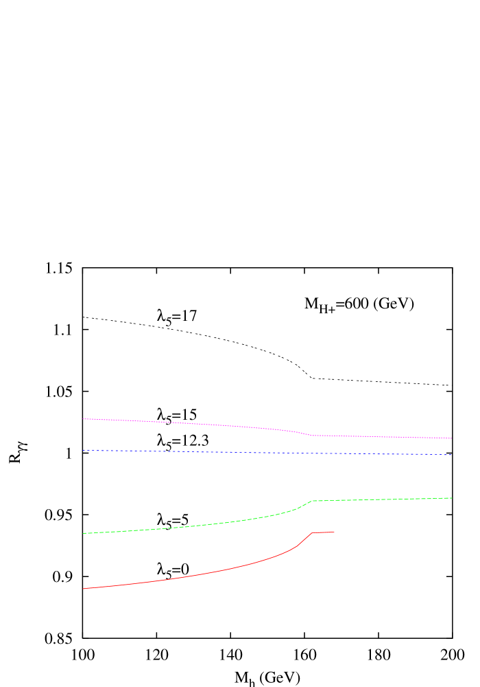
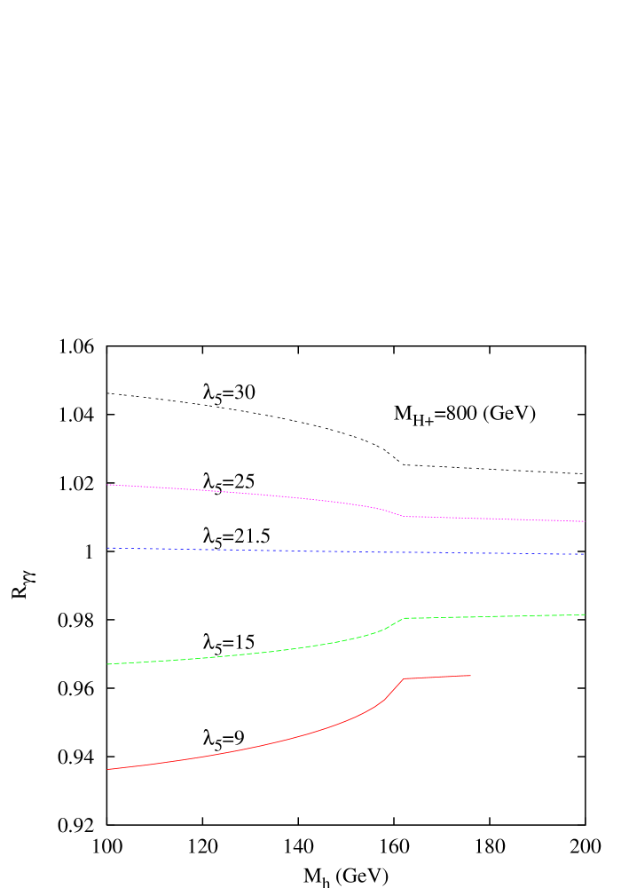
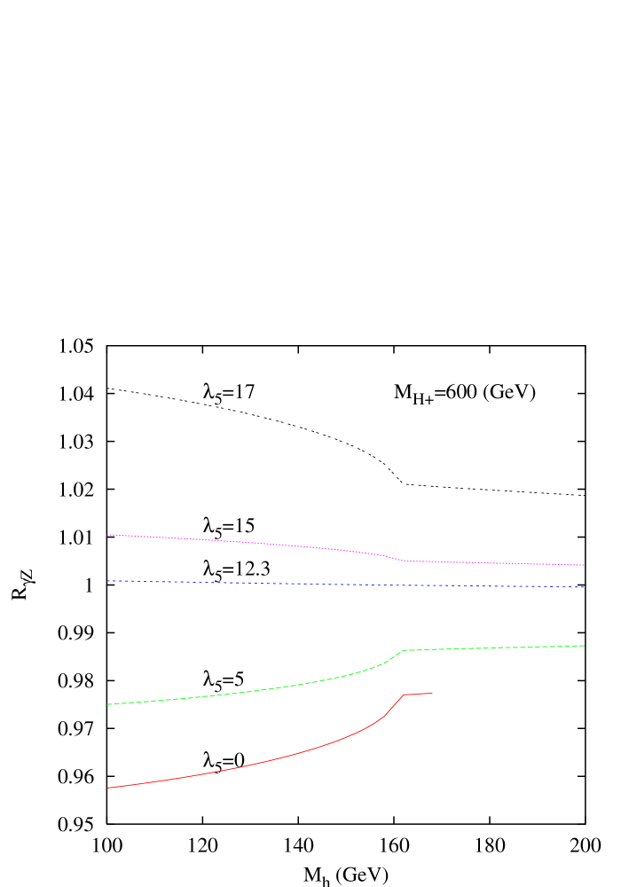
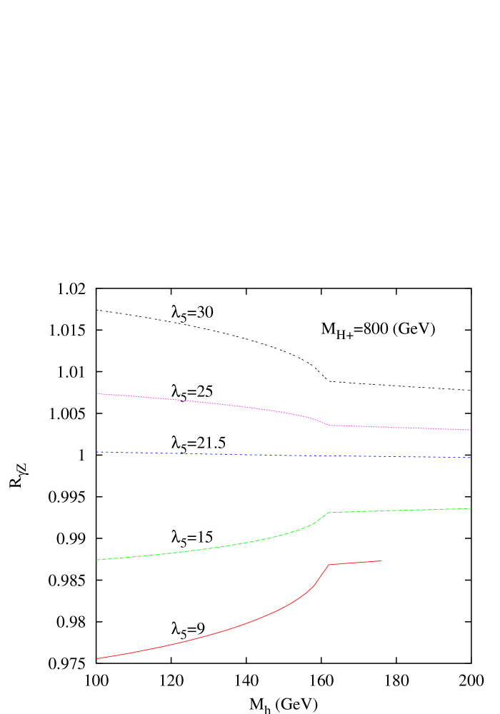
Figure 2: $R_{\gamma\gamma}$ (upper plots) and $R_{\gamma Z}$ (lower plots) as function of $M_{h^{0}}$ for $M_{H^{\pm}}=400$ GeV (left plots), $M_{H^{\pm}}=600$ GeV (middle plots), $M_{H^{\pm}}=800$ GeV (right plots) and $\tan\beta=1$.

For discussion of the non-standard effects, we introduce the following ratios,

$$R_{\gamma V}=\frac{\Gamma(h^{0}\to\gamma V)}{\Gamma(H_{SM}\to\gamma V)}\,,\quad V=\gamma,Z,\ \ {\rm and}\ \ R_{bb}=\frac{\Gamma(h^{0}\to b\bar{b})}{\Gamma(H_{SM}\to b\bar{b})}\,,$$ (20)

which measure the deviations of the various $h^{0}$ partial widths from their SM values with $M_{H_{SM}}=M_{h^{0}}$. In Fig. 2, these ratios are displayed for three values of the charged Higgs mass, for several values of $\lambda_{5}$, and for $\tan\beta\approx 1$. The choice for $\tan\beta$ is motivated by unitarity constraints; the parameter space allowed by unitarity is large for $\tan\beta\approx{\cal O}(1)$ and is reduced for large $\tan\beta$.
In the decoupling regime, the tree level couplings $h^{0}q\bar{q}$ become nearly equal to their SM values, and so the ratios $R_{\gamma V}$ are independent of $\tan\beta$.

As one can see in Fig. 2, for each value of $M_{H^{\pm}}=400,600,800$ GeV one can find corresponding values of $\lambda_{5}^{0}\approx 5.7,12.3,21.5$ , for which the charged-Higgs contribution vanishes, thus yielding $R_{\gamma V}\approx 1$. For $\lambda_{5}$ greater or smaller than the critical values $\lambda_{5}^{0}$, the deviation in the partial width for $h^{0}\to{\gamma\gamma}$ can be as large as $25\%\,(11\%)$ for $M_{H^{\pm}}=400$ GeV (600 GeV). For $M_{H^{\pm}}=800$ GeV, unitarity is violated for $0<\lambda_{5}<9$ and the deviation in $h^{0}\to{\gamma\gamma}$ can be only of the order $\pm 6\%$. We note that our results agree with the results of [22], but some of the parameters chosen in [22] violate the tree-level unitarity constraints. For the ratio $R_{\gamma Z}$, the effect is not so large. The charged-Higgs contribution in this case is decreased by the gauge coupling, which for the $Z$ is smaller than for the photon,

$$\frac{g_{ZH^{+}H^{-}}}{g_{\gamma H^{+}H^{-}}}=\frac{g_{\gamma ZH^{+}H^{-}}}{g_{\gamma\gamma H^{+}H^{-}}}=\frac{(1-2s_{W}^{2})}{(2s_{W}c_{W})}\approx 0.64\,.$$

Only for $M_{H^{\pm}}=400$ GeV and large $\lambda_{5}=17$, the deviation of the ratio $R_{\gamma Z}$ from unity is about 10%.

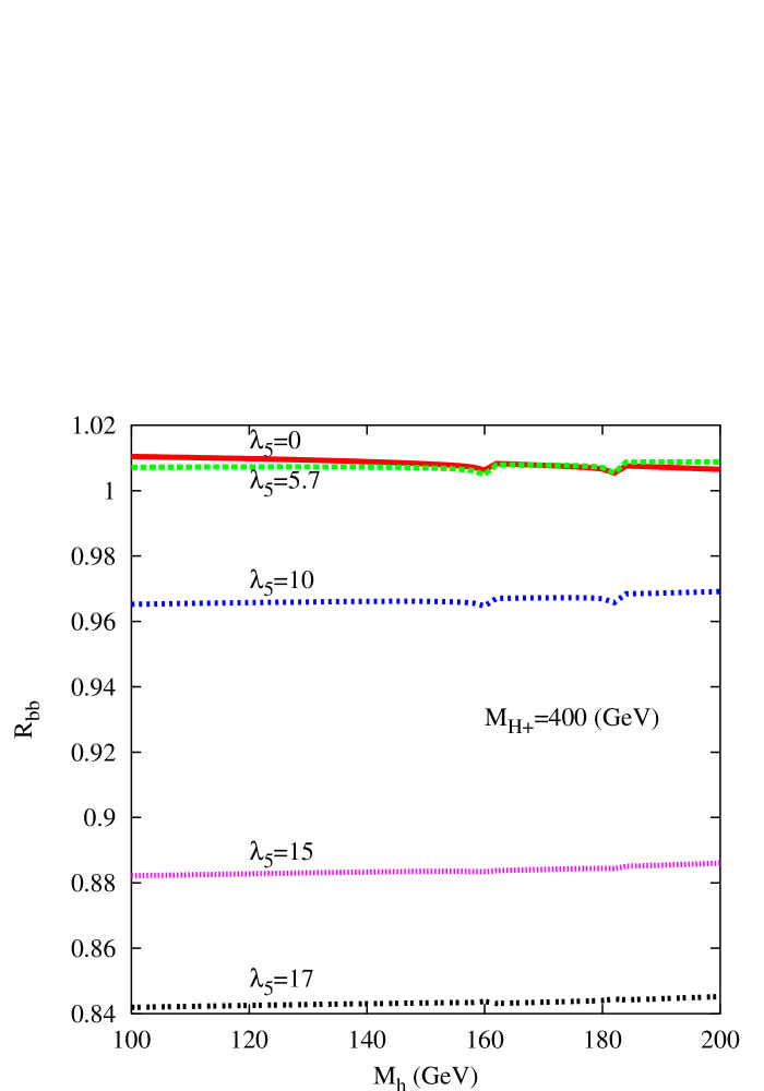
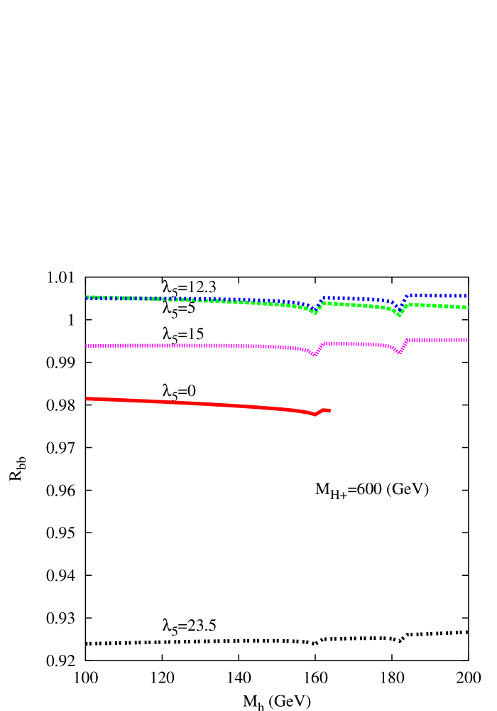
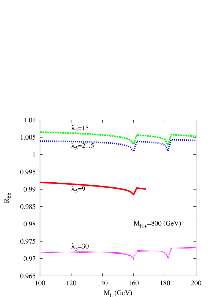
Figure 3: $R_{bb}$ as function of $M_{h^{0}}$ for $M_{H^{\pm}}=400$ GeV (left), $M_{H^{\pm}}=600$ GeV (middle), $M_{H^{\pm}}=800$ GeV (right) and $\tan\beta=1$.

For the Higgs-boson decay into a $b$-quark pair, $h^{0}\to b\bar{b}$, before discussing our numerical results, we would like to mention that we have done the following checks:
i) for the SM case $H_{SM}\to b\bar{b}$, we have reproduced the SM results in perfect agreement with [23], ii) for the THDM case, we have checked numerically that we recover the SM corrections to $H_{SM}\to b\bar{b}$ in the decoupling scenario with all pure THDM couplings set to zero.

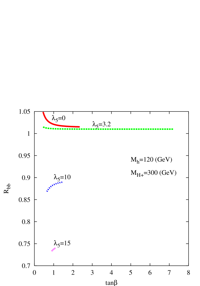
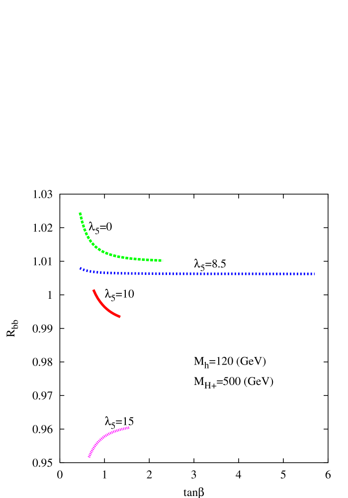
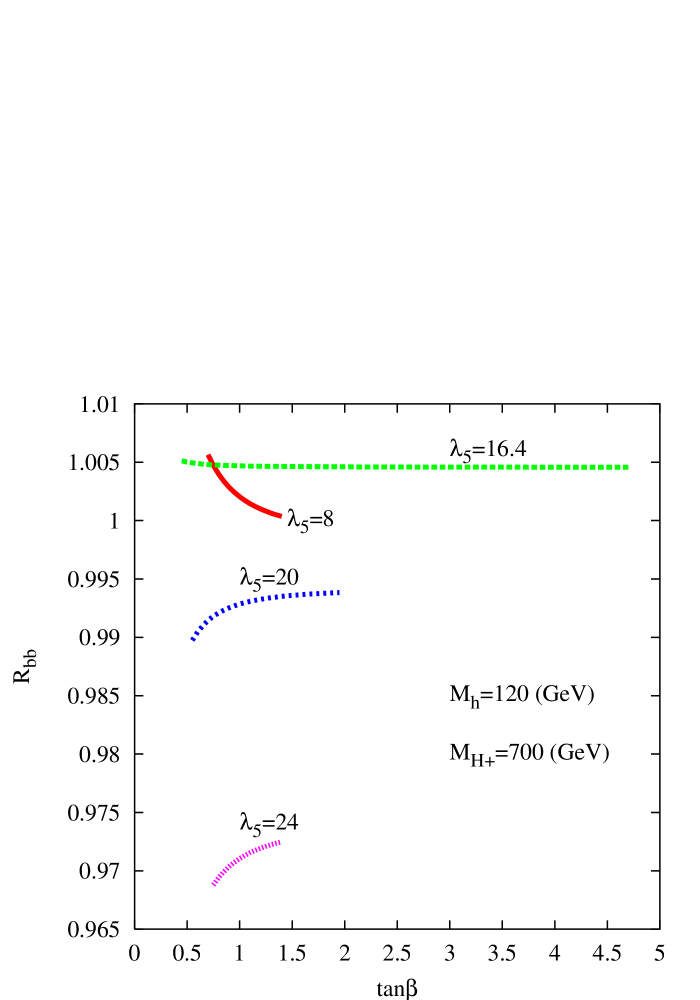
Figure 4: $R_{bb}$ as function of $\tan\beta$ for $M_{H^{\pm}}=300$ GeV (left), $M_{H^{\pm}}=500$ GeV (middle), $M_{H^{\pm}}=700$ GeV (right) and $M_{h^{0}}=120$ GeV.

As explained in the previous section, the Higgs fields are renormalized in the $\overline{\rm MS}$ scheme and hence the result depends on the renormalization scale $\mu_{\overline{\rm MS}}$. This dependence, however, is rather weak for $M_{Z}\leq\mu_{\overline{\rm MS}}\leq M_{t}$, as has been checked explicitly. In the following we will use $\mu_{\overline{\rm MS}}=M_{Z}$.

In Fig. 3, we illustrate the ratio $R_{bb}$ as a function of $M_{h^{0}}$ for the same parameters as applied in the $R_{\gamma V}$ cases. It is clear from this plot that sizeable effects also appear in $h^{0}\to b\bar{b}$, on equal footing as in $h^{0}\to\gamma\gamma$ and $h^{0}\to\gamma Z$. They originate from two sources, allocated to diagrams $d_{1}$ and $d_{2}$ of Fig. 1. The effects from $d_{1}$ are less than 1%, while large effects are due to $d_{2}$. It is interesting to observe that for large values of $\lambda_{5}$ the THDM contribution to $h^{0}\to b\bar{b}$ is reduced with respect to the SM ($R_{bb}<1$). For $M_{H^{\pm}}=400$ GeV ($600$ GeV), the deviation of $\Gamma(h^{0}\to b\bar{b})$ from the SM value can reach 16% for $\lambda_{5}=17$ (resp 8% for $\lambda_{5}=23.5$). For heavy charged Higgs bosons, like $M_{H^{\pm}}=800$ GeV, the deviation is about 3% for $\lambda_{5}=30$.

In the decoupling limit, the $b$-quark mass gets a factor $\tan\beta$ in either the $H^{0}b\bar{b}$, $A^{0}b\bar{b}$, and $H^{-}\bar{b}t$ couplings (see eqs. (17), (18) and (19)), while the top mass gets a factor ${\rm cot}\beta$. Consequently the top (bottom) effect is enhanced for small (large) $\tan\beta$. We have studied the sensitivity to $\tan\beta$, but the unitarity requirements impose severe constraints on $\tan\beta$, which effectively turns out to be of the order one. Note that for $\lambda_{5}\simeq\lambda_{5}^{0}$ no such constraint exists. In Fig. 4, the ratio $R_{bb}$ is displayed as a function of $\tan\beta$ for $M_{h^{0}}=120$ GeV, three values of $M_{H^{\pm}}=300$, 500, 700 GeV, and several values of $\lambda_{5}$. For every value of $M_{H^{\pm}}$ we have chosen $\lambda_{5}$ in such a way that the couplings (1) and (15) vanish, according to (2), and consequently the diagram $d_{2}$ is zero. For $M_{h^{0}}=120$ GeV and $M_{H^{\pm}}=300$, 500, 700 GeV, the zero of (2) is located at $\lambda_{5}=3.2$, 8.5, 16.4, respectively. For those values, the deviation of $h^{0}\to b\bar{b}$ from the SM width arises mainly from diagram $d_{1}$; $R_{bb}$ is not very sensitive to $\tan\beta$, with at most 1% deviations for $0.5\leq\tan\beta\leq 7$. For the other values of $\lambda_{5}$ the effect can be large, but $\tan\beta$ is significantly restricted around unity.

In Fig. 5, we show a contour plot for $\Delta_{\gamma\gamma}=|R_{\gamma\gamma}-1|$ (left panel) and $\Delta_{bb}=|R_{bb}-1|$ (right panel) in the plane $(M_{H^{\pm}},\lambda_{5})$ for $\tan\beta=1$ and $M_{h^{0}}=120$ GeV. The light-grey (yellow) area shows the region where the deviation from the SM value is less than $\pm 3\%$. The solid black line in that region indicates the situations for which the couplings (1) and (15) vanish. In these cases the deviation of the THDM decay widths for $h^{0}\to b\bar{b}$ from the corresponding SM value is less than 1%.

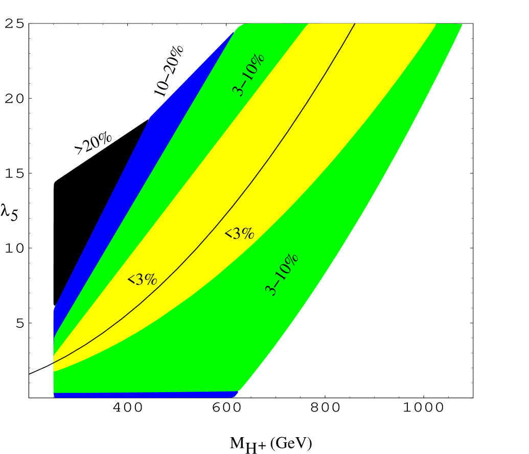
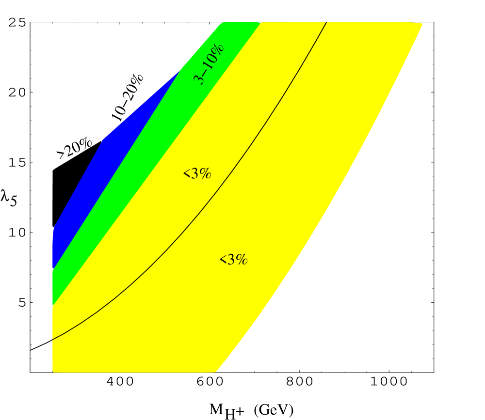
Figure 5: Contours for $\Delta_{\gamma\gamma}=|R_{\gamma\gamma}-1|$ (left panel), $\Delta_{bb}=|R_{bb}-1|$ (right panel) in the $(M_{H^{\pm}},\lambda_{5})$ plane for $M_{h^{0}}=120$ GeV, $\tan\beta=1$ and $\mu_{\overline{\rm MS}}=M_{Z}$

Concerning the left panel, $\Delta_{\gamma\gamma}$, away from the light-grey (yellow) region and for charged Higgs-boson masses $250\mathrel{\raise 1.29167pt\hbox{$<$\kern-7.5pt\lower 4.30554pt\hbox{$\sim$}}}M_{H^{\pm}}\mathrel{\raise 1.29167pt\hbox{$<$\kern-7.5pt\lower 4.30554pt\hbox{$\sim$}}}600$ GeV and $\lambda_{5}\mathrel{\raise 1.29167pt\hbox{$>$\kern-7.5pt\lower 4.30554pt\hbox{$\sim$}}}3$, the deviations are greater than 3% and can become as large as 20% for $M_{H^{\pm}}\mathrel{\raise 1.29167pt\hbox{$<$\kern-7.5pt\lower 4.30554pt\hbox{$\sim$}}}400$ GeV and $\lambda_{5}\mathrel{\raise 1.29167pt\hbox{$>$\kern-7.5pt\lower 4.30554pt\hbox{$\sim$}}}6$. One can also see that for small $\lambda_{5}<1$ and $M_{H^{\pm}}$ below 600 GeV, the deviation is in the range $10-20\%$. For $\Delta_{bb}$, the behaviour is similar. For $250\mathrel{\raise 1.29167pt\hbox{$<$\kern-7.5pt\lower 4.30554pt\hbox{$\sim$}}}M_{H^{\pm}}\mathrel{\raise 1.29167pt\hbox{$<$\kern-7.5pt\lower 4.30554pt\hbox{$\sim$}}}700$ GeV and $\lambda_{5}\mathrel{\raise 1.29167pt\hbox{$>$\kern-7.5pt\lower 4.30554pt\hbox{$\sim$}}}5$, the deviations from the corresponding SM value exceed $3\%$; for $M_{H^{\pm}}\mathrel{\raise 1.29167pt\hbox{$<$\kern-7.5pt\lower 4.30554pt\hbox{$\sim$}}}400$ GeV and $\lambda_{5}\mathrel{\raise 1.29167pt\hbox{$>$\kern-7.5pt\lower 4.30554pt\hbox{$\sim$}}}10$, effects above $20\%$ are found.

4 Conclusions

We have studied the Higgs-boson decays $h^{0}\to\gamma\gamma$, $\gamma Z$ and $b\bar{b}$ in the THDM within the decoupling-regime scenario. We have shown that, even when taking into account unitarity constraints in the scalar sector, both in $h^{0}\to\gamma\gamma$ and $h^{0}\to\gamma Z$ large quantum effects can occur, i.e we have found sizeable differences between these decays and the corresponding decay widths of the SM Higgs boson. For charged Higgs bosons not too heavy, of about $400$ GeV, the deviations in the decay width for $h^{0}\to\gamma\gamma$ ($h^{0}\to\gamma Z$) from the corresponding SM values can reach the order of 25% (10%).

For the dominant Higgs-boson decay into $b$-quark pairs, the partial width $\Gamma(h^{0}\to b\bar{b})$ in the decoupling limit is identical to the SM one at tree level. It turns out that for the same scenarios leading to sizeable effects in the loop-induced bosonic decays, significant quantum effects are also present in $\Gamma(h^{0}\to b\bar{b})$ at one-loop order. Those effects originate mainly from the scalar self-couplings $h^{0}H^{\pm}H^{\mp}$, $h^{0}H^{0}H^{0}$ and $h^{0}A^{0}A^{0}$. For certain regions of the charged Higgs-boson mass and the parameter $\lambda_{5}$, the deviation with respect to the SM value can be also of the order of 25%. Hence, quantum effects in $h^{0}\to b\bar{b}$ can be of the same size as in the $\gamma\gamma,\gamma Z$ decay modes. Therefore, not only the one-loop effects to $h^{0}\to\{\gamma\gamma,\gamma Z\}$ but also the quantum contributions to $h^{0}\to b\bar{b}$ can be used to distinguish between THDM and SM.

At the end, we would like to emphasize, that for large values of the charged Higgs boson masses, unitarity requires large $\lambda_{5}$ (or large $\mu_{12}^{2}$). In this decoupling limit [17], and as it can be seen from the figures, the deviations of the observables we have been considering above from their SM values are very small.

References

- [1] M. W. Grünewald, “Electroweak precision data: Global Higgs analysis”, hep-ex/0304023, Invited talk at Mini-Workshop on Electroweak Precision Data and the Higgs Mass, Zeuthen, Germany, 28 Feb - 1 Mar 2003 (to appear in the Proceedings); Nucl. Phys. Proc. Suppl. 117 (2003) 280 , hep-ex/0210003.
- [2] G. Abbiendi et al., OPAL Collaboration, hep-ex/0209078; P. Achard et al., L3 Collaboration, Phys. Lett. B517, 319 (2001), hep-ex/0107054.
- [3] J.F. Gunion, H.E. Haber, G.L. Kane, S. Dawson, The Higgs Hunter’s Guide (Addison–Wesley, Reading, 1990).
- [4] K. Ackerstaff et al., OPAL Collaboration, Eur. Phys. J. C5 (1998) 19.
- [5] M. Battaglia, K. Desch, Published in *Batavia 2000, Physics and experiments with future linear e+ e- colliders* 163-182, hep-ph/0101165.
- [6] T. Appelquist, J. Carazzone, Phys. Rev. D11, 2856 (1975).
- [7] J.C. Collins, Renormalization, (1984) Cambridge University Press.
- [8] A. Dobado, M. J. Herrero, S. Peñaranda, Eur. Phys. J. C7 (1999) 313, hep-ph/9710313; Eur. Phys. J. C12 (2000) 673, hep-ph/9903211; Eur. Phys. J. C17 (2000) 487, hep-ph/0002134; hep-ph/9711441; hep-ph/9806488.
- [9] M. Drees, K. Hagiwara, Phys. Rev. D42 (1990) 1709; P. Gosdzinsky, J. Solà, Phys. Lett. B254 (1991) 139; L.J. Hall, R. Rattazzi, U. Sarid, Phys. Rev. D50 (1994) 7048, hep-ph/9306309; M. Carenaet al., Nucl. Phys. B577 (2000) 88, hep-ph/9912516, and references therein.
- [10] J.A. Coarasa, R.A. Jiménez, J. Solà, Phys. Lett. B389 (1996) 312; J.A. Coarasa et al., Eur. Phys. J. C2 (1998) 373; S. Alam et al., Phys. Rev. D62 (2000) 095011; A. Belyaev et al., Phys. Rev. D65 (2002) 031701.
- [11] J. Guasch, W. Hollik, S. Peñaranda, Phys. Lett. B515 (2001) 367; M. Carena et al., Phys. Rev. D65 (2002) 055005, Erratum-ibid. D65 (2002) 099902; A. M. Curiel et al., Phys. Rev. D65 (2002) 075006.
- [12] A. Djouadi, V. Driesen, W. Hollik, J. I. Illana, Eur. Phys. J. C1, 149 (1998); A. Djouadi, V. Driesen, W. Hollik, A. Kraft, Eur. Phys. J. C1, 163 (1998); C. S. Huang, X. H. Wu, Phys. Rev. D66 (2002) 075002.
- [13] H. E. Haber et al., Phys. Rev. D63, 055004 (2001); hep-ph/0102169.
- [14] W. Hollik, S. Peñaranda, Eur. Phys. J. C23, 163 (2002); Nucl. Phys. Proc. Suppl. 116 (2003) 311; A. Dobado, M. J. Herrero, W. Hollik, S. Peñaranda, Phys. Rev. D66 (2002) 095016; hep-ph/0210315.
- [15] S. Kanemura et al., Phys. Lett. B558 (2003) 157; hep-ph/0211047.
- [16] H. E. Haber hep-ph/9505240; H. E. Haber et al., hep-ph/0007006, Phys. Rev. D63 (2001) 055004; M. Carena et al., Phys. Rev. D65 (2002) 055005; M. Carena, H.E Haber, hep-ph/0208209.
- [17] J. F. Gunion, H. E. Haber, Phys. Rev. D67 (2003) 075019.
- [18] H. E. Haber, in: Eloisatron Workshop, Erice 1992, Properties of SUSY Particles, p. 321-372, hep-ph/9305248.
- [19] B. W. Lee, C. Quigg, H. B. Thacker, Phys. Rev. Lett. 38, 883 (1977); Phys. Rev. D16, 1519 (1977).
- [20] S. Kanemura, T. Kubota, E. Takasugi, Phys. Lett. B313, 155 (1993); A. G. Akeroyd, A. Arhrib, E. M. Naimi, Phys. Lett. B490, 119 (2000); A. Arhrib, hep-ph/0012353.
- [21] J. M. Cornwall, D. N. Levin, G. Tiktopoulos, Phys. Rev. D10, 1145 (1974), Erratum-ibid. D11, 972 (1975); G. J. Gounaris, R. Kögerler, H. Neufeld, Phys. Rev. D34, 3257 (1986).
- [22] I. F. Ginzburg, M. Krawczyk, P. Osland, Nucl. Instrum. Meth. A 472, 149 (2001).
- [23] A. Dabelstein, W. Hollik, Z. Phys. C 53, 507 (1992); B. A. Kniehl, Nucl. Phys. B376, 3 (1992).
- [24] M. Böhm, H. Spiesberger, W. Hollik, Fortsch. Phys. 34 (1986) 687.
- [25] J. Küblbeck, M. Böhm, A. Denner, Comput. Phys. Commun. 60, 165 (1990); T. Hahn, Comput. Phys. Commun. 140, 418 (2001); T. Hahn, C. Schappacher, Comput. Phys. Commun. 143, 54 (2002); T. Hahn, M. Perez-Victoria, Comput. Phys. Commun. 118, 153 (1999).
- [26] G. J. van Oldenborgh, Comput. Phys. Commun. 66, 1 (1991); T. Hahn, Acta Phys. Polon. B 30, 3469 (1999).
- [27] A. Dabelstein, Nucl. Phys. B456, 25 (1995), hep-ph/9503443.
- [28] M. N. Dubinin, A. V. Semenov, Eur. Phys. J. C28, 223 (2003); R. Santos, A. Barroso, Phys. Rev. D56, 5366 (1997).
- [29] A. Dabelstein, Z. Phys. C 67, 495 (1995); A. Dabelstein, W. Hollik, MPI-PH-93-86; P. Chankowski, S. Pokorski, J. Rosiek, Nucl. Phys. B423, 437 (1994).
- [30] A. Akeroyd, A. Arhrib, E. Naimi, Eur. Phys. J. C20, 51 (2001); A. Arhrib, G. Moultaka, Nucl. Phys. B558, 3 (1999).
- [31] P. Gambino, M. Misiak, Nucl. Phys. B611, 338 (2001); F. M. Borzumati, C. Greub, Phys. Rev. D58, 074004 (1998); ibid Phys. Rev. D59, 057501 (1999); W. S. Hou, R. S. Willey, Phys. Lett. B202, 591 (1988).
- [32] H. E. Haber, H. E. Logan, Phys. Rev. D 62, 015011 (2000).