DESY 03-096 ISSN 0418-9833
hep-ph/0307386
July 2003

$\chi_{c1}$ and $\chi_{c2}$ decay angular distributions at the Fermilab Tevatron

Abstract

We consider the hadroproduction of $\chi_{c1}$ and $\chi_{c2}$ mesons and their subsequent radiative decays to $J/\psi$ mesons and photons in the factorization formalism of nonrelativistic quantum chromodynamics, and study the decay angular distributions, by means of helicity density matrices, in view of their sensitivity to color-octet processes. We present numerical results appropriate for the Fermilab Tevatron.

PACS numbers: 12.38.Bx, 13.60.Le, 13.85.Ni, 14.40.Gx

1 Introduction

Since the discovery of the $J/\psi$ meson in 1974, charmonium has provided a useful laboratory for quantitative tests of quantum chromodynamics (QCD) and, in particular, of the interplay of perturbative and nonperturbative phenomena. The factorization formalism of nonrelativistic QCD (NRQCD) [1] provides a rigorous theoretical framework for the description of heavy-quarkonium production and decay. This formalism implies a separation of short-distance coefficients, which can be calculated perturbatively as expansions in the strong-coupling constant $\alpha_{s}$, from long-distance matrix elements (MEs), which must be extracted from experiment. The relative importance of the latter can be estimated by means of velocity scaling rules, i.e., the MEs are predicted to scale with a definite power of the heavy-quark ($Q$) velocity $v$ in the limit $v\ll 1$. In this way, the theoretical predictions are organized as double expansions in $\alpha_{s}$ and $v$. A crucial feature of this formalism is that it takes into account the complete structure of the $Q\overline{Q}$ Fock space, which is spanned by the states $n={}^{2S+1}L_{J}^{(\zeta)}$ with definite spin $S$, orbital angular momentum $L$, total angular momentum $J$, and color multiplicity $\zeta=1,8$. In particular, this formalism predicts the existence of color-octet (CO) processes in nature. This means that $Q\overline{Q}$ pairs are produced at short distances in CO states and subsequently evolve into physical, color-singlet (CS) quarkonia by the nonperturbative emission of soft gluons. In the limit $v\to 0$, the traditional CS model (CSM) [2] is recovered. The greatest triumph of this formalism was that it was able to correctly describe [3] the cross section of inclusive charmonium hadroproduction measured in $p\overline{p}$ collisions at the Fermilab Tevatron [4], which had turned out to be more than one order of magnitude in excess of the theoretical prediction based on the CSM.

Apart from this phenomenological drawback, the CSM also suffers from severe conceptual problems indicating that it is incomplete. These include the presence of logarithmic infrared divergences in the ${\cal O}(\alpha_{s})$ corrections to $P$-wave decays to light hadrons and in the relativistic corrections to $S$-wave annihilation [5], and the lack of a general argument for its validity in higher orders of perturbation theory. While the $k_{T}$-factorization [6] and hard-comover-scattering [7] approaches manage to bring the CSM prediction much closer to the Tevatron data, they do not cure the conceptual defects of the CSM. The color evaporation model [8], which is intuitive and useful for qualitative studies, also leads to a significantly better description of the Tevatron data, but it is not meant to represent a rigorous framework for perturbation theory. In this sense, a coequal alternative to the NRQCD factorization formalism is presently not available.

In order to convincingly establish the phenomenological significance of the CO processes, it is indispensable to identify them in other kinds of high-energy experiments as well. Studies of charmonium production in $ep$ photoproduction, $ep$ and $\nu N$ deep-inelastic scattering (DIS), $e^{+}e^{-}$ annihilation, $\gamma\gamma$ collisions, and $b$-hadron decays may be found in the literature; see Ref. [9] and references cited therein. Furthermore, the polarization of $\psi^{\prime}$ mesons produced directly and of $J/\psi$ mesons produced promptly, i.e., either directly or via the feed-down from heavier charmonia, which also provides a sensitive probe of CO processes, was investigated [10, 11, 12, 13]. Until very recently, none of these studies was able to prove or disprove the NRQCD factorization hypothesis. However, H1 data of $ep\to eJ/\psi+X$ in DIS at HERA [14] and DELPHI data of $\gamma\gamma\to J/\psi+X$ at LEP2 [15] provide first independent evidence for it [16, 17].

The cross section ratio of $\chi_{c1}$ and $\chi_{c2}$ inclusive hadroproduction was measured by the CDF Collaboration in Run 1 at the Tevatron [18]. The $\chi_{cJ}$ mesons were detected through their radiative decays to $J/\psi$ mesons and photons. The $J/\psi$ mesons were identified via their decay to $\mu^{+}\mu^{-}$ pairs, and the photons were reconstructed through their conversion to $e^{+}e^{-}$ pairs, which provide an excellent energy resolution for the primary photons. The increased data sample to be collected during Run 2, which has just started, will allow for more detailed investigations of these cross sections, including the angular distributions of the $\chi_{cJ}$ decay products. The latter carry all the information on the $\chi_{cJ}$ polarization and thus provide a handle on the CO processes.

In this paper, we study the angular distributions of the processes $p\overline{p}\to\chi_{cJ}+X$ ($J=1,2$) with subsequent decays $\chi_{cJ}\to J/\psi\gamma$ with regard to their power to distinguish between NRQCD and the CSM. Specifically, we consider the polar and azimuthal angles, $\theta$ and $\phi$, of the $J/\psi$ meson in the $\chi_{cJ}$ rest frame. Once a suitable coordinate system is defined in that frame, the full angular information is encoded in the helicity density matrix $\rho_{\lambda\lambda^{\prime}}^{J}$ of the primary $\chi_{cJ}$ production process, where $\lambda$ and $\lambda^{\prime}$ denote the $\chi_{cJ}$ helicities. The matrix $\rho_{\lambda\lambda^{\prime}}^{J}$, therefore, provides a systematic way of analyzing the complicated details of the $\theta$ and $\phi$ dependences. In the following, we study $\rho_{\lambda\lambda^{\prime}}^{J}$ in four commonly used polarization frames as functions of the $\chi_{cJ}$ transverse momentum $p_{T}$ so as to identify optimal observables to discriminate NRQCD from the CSM.

This paper is organized as follows. In Sec. 2, we list the formulas necessary to evaluate the helicity density matrix of $p\overline{p}\to\chi_{cJ}+X\to J/\psi\gamma+X$ for $J=1,2$. In Sec. 3, we present our numerical results and discuss their phenomenological implications. Our conclusions are summarized in Sec. 4.

2 Analytic results

We consider the production processes $p\overline{p}\to\chi_{cJ}j+X$, where $J=1,2$ and $j$ denotes a hadron jet, followed by the radiative decays $\chi_{cJ}\to J/\psi\gamma$ in the narrow-width approximation. (The presence of the hadron jet, which does not have to be observed, allows for the $\chi_{cJ}$ meson to have finite transverse momentum.) Let $\sqrt{S}$ be the center-of-mass energy of the hadronic collision, $M$ the mass of the $\chi_{cJ}$ meson, $p_{T}$ the transverse momentum common to the $\chi_{cJ}$ meson and the jet, $y$ and $y_{j}$ the rapidities of the latter, $\lambda=-J,\ldots,J$ the helicity of the $\chi_{cJ}$ meson in some polarization frame, and $\theta$ and $\phi$ the polar and azimuthal angles of the $J/\psi$ meson in the respective coordinate system defined in the $\chi_{cJ}$ rest frame. Then, the differential cross section can be written as

$$\frac{d^{5}\sigma^{J}}{dp_{T}^{2}\,dy\,dy_{j}\,d^{2}\Omega}=B_{J}\sum_{\lambda,\lambda^{\prime}=-J}^{J}\frac{d^{3}\rho_{\lambda\lambda^{\prime}}^{J}}{dp_{T}^{2}\,dy\,dy_{j}}A_{\lambda\lambda^{\prime}}^{J}(\theta,\phi),$$ (1)

where $\rho_{\lambda\lambda^{\prime}}^{J}$ and $A_{\lambda\lambda^{\prime}}^{J}$ refer to the production and decay processes, respectively, $B_{J}$ denotes the branching fraction of $\chi_{cJ}\to J/\psi\gamma$, and $d^{2}\Omega=d\cos\theta\,d\phi$. Invoking the factorization theorems of the QCD parton model and NRQCD, we have

$$\frac{d^{3}\rho_{\lambda\lambda^{\prime}}^{J}}{dp_{T}^{2}\,dy\,dy_{j}}=\sum_{a,b,d,n}x_{a}f_{a/p}(x_{a},\mu_{f})x_{b}f_{b/\overline{p}}(x_{b},\mu_{f})\langle{\cal O}^{\chi_{cJ}}[n]\rangle\frac{1}{16\pi s}\rho_{\lambda\lambda^{\prime}}\left(ab\to c\overline{c}[n]d\right).$$ (2)

Here, it is summed over the active partons $a,b,d=g,q,\overline{q}$ and the $c\overline{c}$ Fock states $n$, $f_{a/h}(x_{a},\mu_{f})$ are the PDFs of the beam hadron $h$, $x_{a}$ is the fraction of longitudinal momentum that $a$ receives from $h$, $\mu_{f}$ is the factorization scale, $\langle{\cal O}^{\chi_{cJ}}[n]\rangle$ are the MEs of the $\chi_{cJ}$ meson, and

$$\rho_{\lambda\lambda^{\prime}}\left(ab\to c\overline{c}[n]d\right)=\sum{\cal T}^{\star}\left(ab\to c\overline{c}[n,\lambda^{\prime}]d\right){\cal T}\left(ab\to c\overline{c}[n,\lambda]d\right),$$ (3)

where it is averaged (summed) over the spin and color states of $a$ and $b$ ($d$), and ${\cal T}$ denotes the transition-matrix element. We have

$$x_{a,b}=\frac{m_{T}\exp(\pm y)+p_{T}\exp(\pm y_{j})}{\sqrt{S}},$$ (4)

where $m_{T}=\sqrt{M^{2}+p_{T}^{2}}$ is the transverse mass of the $\chi_{cJ}$ meson. The partonic Mandelstam variables $s=(p_{a}+p_{b})^{2}$, $t=(p_{a}-P)^{2}$, and $u=(p_{b}-P)^{2}$, where $P$ is the four-momentum of the $\chi_{cJ}$ meson, can be expressed in terms of $p_{T}$, $y$, and $y_{j}$ as

$$s = p_{T}^{2}+m_{T}^{2}+2p_{T}m_{T}\cosh(y-y_{j}),$$

$$t = -p_{T}^{2}-p_{T}m_{T}\exp(y_{j}-y),$$

$$u = -p_{T}^{2}-p_{T}m_{T}\exp(y-y_{j}),$$ (5)

respectively. Notice that $s+t+u=M^{2}$ and $sp_{T}^{2}=tu$. The kinematically allowed ranges of $p_{T}$, $y$, and $y_{j}$ are

$$0 \leq p_{T}\leq\frac{S-M^{2}}{2\sqrt{S}},$$

$$|y| \leq \mathop{\mbox{arcosh}}\nolimits\frac{S+M^{2}}{2\sqrt{S}m_{T}},$$

$$-\ln\frac{\sqrt{S}-m_{T}\exp(-y)}{p_{T}} \leq y_{j}\leq\ln\frac{\sqrt{S}-m_{T}\exp(y)}{p_{T}}.$$ (6)

Integrating Eq. (1) over $y_{j}$, we obtain the inclusive cross section of $p\overline{p}\to\chi_{cJ}+X$.

Choosing a suitable coordinate system in the $\chi_{cJ}$ rest frame and defining

$$\langle\lambda_{1},\lambda_{2},\theta,\phi|T|J,\lambda\rangle = {\cal T}(\chi_{cJ}(\lambda)\to J/\psi(\lambda_{1},\theta,\phi)\gamma(\lambda_{2},\pi-\theta,\phi+\pi)),$$

$$T_{\lambda_{1}\lambda_{2}}^{J} = \sqrt{\frac{4\pi}{2J+1}}\left.\langle\lambda_{1},\lambda_{2},0,0|T|J,\lambda\rangle\right|_{\lambda=\lambda_{1}-\lambda_{2}},$$ (7)

where $\lambda_{1}=0,\pm 1$ and $\lambda_{2}=\pm 1$ are the helicities of the $J/\psi$ and $\gamma$ bosons, respectively, the decay angular distribution is encoded in the matrix

$$A_{\lambda\lambda^{\prime}}^{J}(\theta,\phi)=\frac{\sum_{\lambda_{1},\lambda_{2}}\langle\lambda_{1},\lambda_{2},\theta,\phi|T|J,\lambda^{\prime}\rangle^{\star}\langle\lambda_{1},\lambda_{2},\theta,\phi|T|J,\lambda\rangle}{\sum_{\lambda_{1},\lambda_{2}}|T_{\lambda_{1}\lambda_{2}}^{J}|^{2}}.$$ (8)

This expression may be conveniently evaluated by observing that [19]

$$\langle\lambda_{1},\lambda_{2},\theta,\phi|T|J,\lambda\rangle=\sqrt{\frac{2J+1}{4\pi}}D_{\lambda,\lambda_{1}-\lambda_{2}}^{J\star}(-\phi,\theta,\phi)T_{\lambda_{1}\lambda_{2}}^{J},$$ (9)

where $D_{m^{\prime}m}^{j}(\alpha,\beta,\gamma)=\langle j,m^{\prime}|D(\alpha,\beta,\gamma)|j,m\rangle$ is the representation of the rotation operator $D(\alpha,\beta,\gamma)=\exp(-i\gamma J_{z})\exp(-i\beta J_{y})\exp(-i\alpha J_{z})$, with $\alpha$, $\beta$, and $\gamma$ being the Euler angles, in the eigenstates $|j,m\rangle$ of ${\boldmath J}^{2}$ and $J_{z}$. We have

$$D_{m^{\prime}m}^{j}(\alpha,\beta,\gamma)=\exp(-i\gamma m^{\prime})d_{m^{\prime}m}^{j}(\beta)\exp(-i\alpha m),$$ (10)

where $d_{m^{\prime}m}^{j}(\beta)=\langle j,m^{\prime}|\exp(-i\beta J_{y})|j,m\rangle$ are the well-known $d$ functions, which may be evaluated from Wigner’s formula [20]

$$d_{m^{\prime}m}^{j}(\beta) = \sum_{k=\max(0,m-m^{\prime})}^{\min(j+m,j-m^{\prime})}(-1)^{k-m+m^{\prime}}\frac{\sqrt{(j+m)!(j-m)!(j+m^{\prime})!(j-m^{\prime})!}}{k!(k-m+m^{\prime})!(j+m-k)!(j-m^{\prime}-k)!}$$ (11)

$${}\times\left(\cos\frac{\beta}{2}\right)^{2j+m-m^{\prime}-2k}\left(\sin\frac{\beta}{2}\right)^{2k-m+m^{\prime}}.$$

Owing to the orthogonality relation

$$\int d^{2}\Omega D_{m^{\prime}m^{\prime\prime}}^{j}(-\phi,\theta,\phi)D_{mm^{\prime\prime}}^{j\star}(-\phi,\theta,\phi)=\frac{4\pi}{2j+1}\delta_{m^{\prime}m},$$ (12)

$A_{\lambda\lambda^{\prime}}^{J}$ is normalized as

$$\int d^{2}\Omega A_{\lambda\lambda^{\prime}}^{J}(\theta,\phi)=\delta_{\lambda\lambda^{\prime}},$$ (13)

so that, upon integration over the solid angle, Eq. (1) reduces to the unpolarized narrow-width approximation formula

$$\frac{d^{3}\sigma}{dp_{T}^{2}\,dy\,dy_{j}}\left(p\overline{p}\to\chi_{cJ}(\to J/\psi\gamma)j+X\right)=B(\chi_{cJ}\to J/\psi\gamma)\frac{d^{3}\sigma}{dp_{T}^{2}\,dy\,dy_{j}}\left(p\overline{p}\to\chi_{cJ}j+X\right).$$ (14)

By definition, the helicity density matrix $\rho_{\lambda\lambda^{\prime}}^{J}$ is hermitian, $\rho_{\lambda^{\prime}\lambda}^{J\star}=\rho_{\lambda\lambda^{\prime}}^{J}$. Furthermore, invariance of the ${\cal T}$ matrix under reflection in the production plane, by action of the operator ${\cal Y}=\exp(-i\pi J_{y}){\cal P}$, where ${\cal P}$ is the parity operator, leads to the symmetry property $\rho_{-\lambda,-\lambda^{\prime}}^{J}=(-1)^{\lambda-\lambda^{\prime}}\rho_{\lambda\lambda^{\prime}}^{J}$ [19]. Thanks to these constraints, the number of independent real quantities contained in $\rho_{\lambda\lambda^{\prime}}^{J}$ is 5 for $J=1$ and 13 for $J=2$. We may select the entries $\rho_{\lambda\lambda^{\prime}}^{J}$ with $\lambda=0,\dots,J$ and $\lambda^{\prime}=-\lambda,\ldots,\lambda$, noticing that they are real if $|\lambda^{\prime}|=\lambda$.

As for the decay amplitude $T_{\lambda_{1}\lambda_{2}}^{J}$, angular-momentum conservation imposes the selection rule $|\lambda_{1}-\lambda_{2}|\leq J$. Furthermore, parity conservation entails the symmetry property [19]

$$T_{-\lambda_{1},-\lambda_{2}}^{J} = \eta\eta_{1}\eta_{2}(-1)^{J_{1}+J_{2}-J}T_{\lambda_{1}\lambda_{2}}^{J}$$ (15)

$$= (-1)^{J}T_{\lambda_{1}\lambda_{2}}^{J},$$

where $\eta$, $\eta_{1}$, and $\eta_{2}$ ($J$, $J_{1}$, and $J_{2}$) are the parity (total-angular-momentum) quantum numbers of the $\chi_{cJ}$, $J/\psi$, and $\gamma$ bosons, respectively. An independent set of $T_{\lambda_{1}\lambda_{2}}^{J}$ amplitudes thus reads

$$t_{0}^{1} = T_{1,1}^{1}=-T_{-1,-1}^{1},$$

$$t_{1}^{1} = T_{0,-1}^{1}=-T_{0,1}^{1},$$

$$t_{0}^{2} = T_{1,1}^{2}=T_{-1,-1}^{2},$$

$$t_{1}^{2} = T_{0,-1}^{2}=T_{0,1}^{2},$$

$$t_{2}^{2} = T_{1,-1}^{2}=T_{-1,1}^{2}.$$ (16)

Using these ingredients, we can now work out the general form of the angular distributions of the $J/\psi$ meson,

$$W^{J}(\theta,\phi)=\sum_{\lambda,\lambda^{\prime}=-J}^{J}\rho_{\lambda\lambda^{\prime}}^{J}A_{\lambda\lambda^{\prime}}^{J}(\theta,\phi).$$ (17)

We find

$$W^{1}(\theta,\phi) = \frac{3}{4\pi}\left\{\rho_{0,0}^{1}\left[r_{0}^{1}\cos^{2}\theta+\frac{r_{1}^{1}}{2}\sin^{2}\theta\right]+\rho_{1,1}^{1}\left[r_{0}^{1}\sin^{2}\theta+\frac{r_{1}^{1}}{2}(1+\cos^{2}\theta)\right]\right.$$

$${}-\left.\sqrt{2}\mathop{\mbox{Re}}\nolimits\rho_{1,0}^{1}\left(2r_{0}^{1}-r_{1}^{1}\right)\sin\theta\cos\theta\cos\phi-\rho_{1,-1}^{1}\left(r_{0}^{1}-\frac{r_{1}^{1}}{2}\right)\sin^{2}\theta\cos(2\phi)\right\},$$

$$W^{2}(\theta,\phi) = \frac{5}{4\pi}\left\{\frac{\rho_{0,0}^{2}}{2}\left[\frac{r_{0}^{2}}{2}(1-3\cos^{2}\theta)^{2}+3r_{1}^{2}\sin^{2}\theta\cos^{2}\theta+\frac{3}{4}r_{2}^{2}\sin^{4}\theta\right]\right.$$ (18)

$${}+\rho_{1,1}^{2}\left[3r_{0}^{2}\sin^{2}\theta\cos^{2}\theta+\frac{r_{1}^{2}}{2}(1-3\cos^{2}\theta+4\cos^{4}\theta)+\frac{r_{2}^{2}}{2}\sin^{2}\theta(1+\cos^{2}\theta)\right]$$

$${}+\rho_{2,2}^{2}\left[\frac{3}{4}r_{0}^{2}\sin^{4}\theta+\frac{r_{1}^{2}}{2}\sin^{2}\theta(1+\cos^{2}\theta)+\frac{r_{2}^{2}}{8}(1+6\cos^{2}\theta+\cos^{4}\theta)\right]$$

$${}+\sqrt{6}\mathop{\mbox{Re}}\nolimits\rho_{1,0}^{2}\left[r_{0}^{2}(1-3\cos^{2}\theta)-r_{1}^{2}(1-2\cos^{2}\theta)+\frac{r_{2}^{2}}{2}\sin^{2}\theta\right]\sin\theta\cos\theta\cos\phi$$

$${}-\mathop{\mbox{Re}}\nolimits\rho_{2,1}^{2}\left[3r_{0}^{2}\sin^{2}\theta+2r_{1}^{2}\cos^{2}\theta-\frac{r_{2}^{2}}{2}(3+\cos^{2}\theta)\right]\sin\theta\cos\theta\cos\phi$$

$${}-\rho_{1,-1}^{2}\left[3r_{0}^{2}\cos^{2}\theta+\frac{r_{1}^{2}}{2}(1-4\cos^{2})-\frac{r_{2}^{2}}{2}\sin^{2}\theta\right]\sin^{2}\theta\cos(2\phi)$$

$${}-\sqrt{6}\mathop{\mbox{Re}}\nolimits\rho_{2,0}^{2}\left[\frac{r_{0}^{2}}{2}(1-3\cos^{2}\theta)+r_{1}^{2}\cos^{2}\theta-\frac{r_{2}^{2}}{4}(1+\cos^{2}\theta)\right]\sin^{2}\theta\cos(2\phi)$$

$${}+\mathop{\mbox{Re}}\nolimits\rho_{2,-1}^{2}\left(3r_{0}^{2}-2r_{1}^{2}+\frac{r_{2}^{2}}{2}\right)\sin^{3}\theta\cos\theta\cos(3\phi)$$

$${}+\left.\frac{\rho_{2,-2}^{2}}{2}\left(\frac{3}{2}r_{0}^{2}-r_{1}^{2}+\frac{r_{2}^{2}}{4}\right)\sin^{4}\theta\cos(4\phi)\right\},$$

where

$$r_{\lambda}^{J}=\frac{\left|t_{\lambda}^{J}\right|^{2}}{\sum_{\lambda^{\prime}=0}^{J}\left|t_{\lambda^{\prime}}^{J}\right|^{2}}$$ (19)

are positive numbers satisfying $\sum_{\lambda=0}^{J}r_{\lambda}^{J}=1$ to be determined experimentally. In fact, the Fermilab E835 Collaboration [21] studied the angular distributions of the exclusive reactions $p\overline{p}\to\chi_{cJ}\to J/\psi\gamma\to e^{+}e^{-}\gamma$, with $J=1,2$, and measured the fractional amplitudes of the electric dipole (E1), magnetic quadrupole (M2), and electric octupole (E3) transitions. They found the E1 transition to dominate, as expected from theoretical considerations. From their results, we extract the values

$$r_{0}^{1} = 0.498\pm 0.032,\qquad r_{1}^{1}=0.502\pm 0.032,$$

$$r_{0}^{2} = 0.075\pm 0.029,\qquad r_{1}^{2}=0.250\pm 0.048,\qquad r_{2}^{2}=0.674\pm 0.052.$$ (20)

The corresponding values for a pure E1 transition read $r_{0}^{1}=r_{1}^{1}=0.5$, $r_{0}^{2}=0.1$, $r_{1}^{2}=0.3$, and $r_{2}^{2}=0.6$.

We work in the fixed-flavor-number scheme, i.e., we have $n_{f}=3$ active quark flavors $q=u,d,s$ in the proton and antiproton. As required by parton-model kinematics, we treat the quarks $q$ as massless. The charm quark $c$ and antiquark $\overline{c}$ only appear in the final state. We are thus led to consider the following partonic subprocesses:

$$gg \to c\overline{c}[n]g,$$

$$gq \to c\overline{c}[n]q,$$

$$q\overline{q} \to c\overline{c}[n]g.$$ (21)

As for the $\chi_{cJ}$ mesons, the $c\overline{c}$ Fock states contributing at LO in $v$ are $n={}^{3}\!P_{J}^{(1)},{}^{3}\!S_{1}^{(8)}$. Their MEs satisfy the multiplicity relations

$$\left\langle{\cal O}^{\chi_{cJ}}\left[{}^{3}\!P_{J}^{(1)}\right]\right\rangle = (2J+1)\left\langle{\cal O}^{\chi_{c0}}\left[{}^{3}\!P_{0}^{(1)}\right]\right\rangle,$$

$$\left\langle{\cal O}^{\chi_{cJ}}\left[{}^{3}\!S_{1}^{(8)}\right]\right\rangle = (2J+1)\left\langle{\cal O}^{\chi_{c0}}\left[{}^{3}\!S_{1}^{(8)}\right]\right\rangle,$$ (22)

which follow to LO in $v$ from heavy-quark spin symmetry.

Depending on the value of $J$, the partonic helicity density matrices defined in Eq. (3) may be decomposed as

$$\rho_{\lambda\lambda^{\prime}}\left(ab\to c\overline{c}\left[{}^{2S+1}L_{1}^{(\zeta)}\right]d\right) = \epsilon_{\mu}^{\star}(\lambda)\epsilon_{\nu}(\lambda^{\prime})F\left[c_{1}g^{\mu\nu}+c_{2}p_{a}^{\mu}p_{a}^{\nu}+c_{3}p_{b}^{\mu}p_{b}^{\nu}+\frac{c_{4}}{2}\left(p_{a}^{\mu}p_{b}^{\nu}+p_{a}^{\nu}p_{b}^{\mu}\right)\right],$$

$$\rho_{\lambda\lambda^{\prime}}\left(ab\to c\overline{c}\left[{}^{2S+1}L_{2}^{(\zeta)}\right]d\right) = \epsilon_{\mu\nu}^{\star}(\lambda)\epsilon_{\rho\sigma}(\lambda^{\prime})F\left[c_{1}g^{\mu\rho}g^{\nu\sigma}+c_{2}g^{\mu\rho}p_{a}^{\nu}p_{a}^{\sigma}+c_{3}g^{\mu\rho}p_{b}^{\nu}p_{b}^{\sigma}\vphantom{\frac{c_{9}}{2}}\right.$$ (23)

$${}+\frac{c_{4}}{2}g^{\mu\rho}\left(p_{a}^{\nu}p_{b}^{\sigma}+p_{a}^{\sigma}p_{b}^{\nu}\right)+c_{5}p_{a}^{\mu}p_{a}^{\nu}p_{a}^{\rho}p_{a}^{\sigma}+c_{6}p_{b}^{\mu}p_{b}^{\nu}p_{b}^{\rho}p_{b}^{\sigma}$$

$${}+\frac{c_{7}}{2}p_{a}^{\mu}p_{a}^{\rho}\left(p_{a}^{\nu}p_{b}^{\sigma}+p_{a}^{\sigma}p_{b}^{\nu}\right)+\frac{c_{8}}{2}p_{b}^{\mu}p_{b}^{\rho}\left(p_{b}^{\nu}p_{a}^{\sigma}+p_{b}^{\sigma}p_{a}^{\nu}\right)$$

$${}+\left.\frac{c_{9}}{2}\left(p_{a}^{\mu}p_{a}^{\nu}p_{b}^{\rho}p_{b}^{\sigma}+p_{a}^{\rho}p_{a}^{\sigma}p_{b}^{\mu}p_{b}^{\nu}\right)+c_{10}p_{a}^{\mu}p_{b}^{\nu}p_{a}^{\rho}p_{b}^{\sigma}\right],$$

where $\epsilon^{\mu}(\lambda)$ ($\epsilon^{\mu\nu}(\lambda)$) is the polarization vector (tensor) of a $J=1$ ($J=2$) boson with mass $M$, four-momentum $P$, and helicity $\lambda$, and $F$ and $c_{i}$ are functions of the partonic mandelstam variables $s$, $t$, and $u$. Since we work at the tree level, $F$ and $c_{i}$ are real, so that the imaginary parts of $\rho_{\lambda\lambda^{\prime}}^{J}$ all arise from $\epsilon^{\mu}(\lambda)$ and $\epsilon^{\mu\nu}(\lambda)$. The functions $F$ and $c_{i}$ for processes (21) with $n={}^{3}\!P_{1}^{(1)},{}^{3}\!P_{2}^{(1)}$ are listed in the Appendix of Ref. [13]. The results for $n={}^{3}\!S_{1}^{(8)}$ may be found in Eqs. (B27)–(B31), (B39)–(B43), and (B51)–(B55) of Ref. [11], where one has to identify $c_{1}=a$, $c_{2}=M^{2}b$, $c_{3}=M^{2}c$, and $c_{4}=2M^{2}d$.

Lorentz-covariant expressions for $\epsilon^{\mu}(\lambda)$ in four commonly used polarization frames, namely, the recoil, Gottfried-Jackson, target, and Collins-Soper frames, may be found in Ref. [22]. These frames differ in the way $\epsilon^{\mu}(0)$ is fixed. In the $\chi_{cJ}$ rest frame, where $\epsilon^{\mu}(0)=(0,\mbox{\boldmath$\epsilon$}(0))$, we have $\mbox{\boldmath$\epsilon$}(0)=-\mbox{\boldmath$\hat{p}$}$, where $p=p_{p}+p_{\overline{p}}$, in the recoil frame; $\mbox{\boldmath$\epsilon$}(0)=\mbox{\boldmath$\hat{p}_{p}$}$ in the Gottfried-Jackson frame; $\mbox{\boldmath$\epsilon$}(0)=-\mbox{\boldmath$\hat{p}_{\overline{p}}$}$ in the target frame; and $\mbox{\boldmath$\epsilon$}(0)=\left(\mbox{\boldmath$\hat{p}_{p}$}-\mbox{\boldmath$\hat{p}_{\overline{p}}$}\right)/\sqrt{2\left(1-\mbox{\boldmath$\hat{p}_{p}$}\cdot\mbox{\boldmath$\hat{p}_{\overline{p}}$}\right)}$ in the Collins-Soper frame. Here, $\mbox{\boldmath$\hat{p}$}=\mbox{\boldmath$p$}/|\mbox{\boldmath$p$}|$ denotes the unit three-vector. With the help of the addition theorem for two angular momenta, $\epsilon^{\mu\nu}(\lambda)$ can be constructed from the polarization four-vectors of two $J=1$ bosons with the same four-momentum as [23]

$$\epsilon^{\mu\nu}(\lambda)=\sum_{\lambda_{1},\lambda_{2}=-1}^{1}\langle 1,\lambda_{1};1,\lambda_{2}|2,\lambda\rangle\epsilon^{\mu}(\lambda_{1})\epsilon^{\nu}(\lambda_{2}),$$ (24)

where $\langle 1,\lambda_{1};1,\lambda_{2}|2,\lambda\rangle$ are Clebsch-Gordon coefficients. We have $P_{\mu}\epsilon^{\mu}(\lambda)=P_{\mu}\epsilon^{\mu\nu}(\lambda)=g_{\mu\nu}\epsilon^{\mu\nu}(\lambda)=0$ and $\epsilon^{\mu\nu}(\lambda)=\epsilon^{\nu\mu}(\lambda)$.

3 Numerical results

We are now in a position to present our numerical results. We first describe our theoretical input and the kinematic conditions. We use $m_{c}=M/2=(1.5\pm 0.1)$ GeV and the LO formula for $\alpha_{s}^{(n_{f})}(\mu_{r})$ with $n_{f}=3$ [24]. As for the proton PDFs, we employ the LO set by Martin, Roberts, Stirling, and Thorne (MRST98LO) [25], with asymptotic scale parameter $\Lambda^{(4)}=174$ MeV, as our default and the LO set by the CTEQ Collaboration (CTEQ5L) [26], with $\Lambda^{(4)}=192$ MeV, for comparison. The corresponding values of $\Lambda^{(3)}$ are 204 MeV and 224 MeV, respectively. We choose the renormalization and factorization scales to be $\mu_{i}=\xi_{i}m_{T}$, with $i=r,f$, respectively, and independently vary the scale parameters $\xi_{r}$ and $\xi_{f}$ between 1/2 and 2 about the default value 1. We adopt the values of $\left\langle{\cal O}^{\chi_{c0}}\left[{}^{3}\!P_{0}^{(1)}\right]\right\rangle$ and $\left\langle{\cal O}^{\chi_{c0}}\left[{}^{3}\!S_{1}^{(8)}\right]\right\rangle$ from Ref. [12]. Specifically, the former was extracted from the measured partial decay widths of $\chi_{c2}\to\gamma\gamma$ [24], while the latter was fitted to the $p_{T}$ distribution of $\chi_{cJ}$ inclusive hadroproduction [4] and the cross-section ratio $\sigma_{\chi_{c2}}/\sigma_{\chi_{c1}}$ [18] measured at the Tevatron. For set MRST98LO, these values read $\left\langle{\cal O}^{\chi_{c0}}\left[{}^{3}\!P_{0}^{(1)}\right]\right\rangle=(8.9\pm 1.3)\times 10^{-2}$ GeV⁵ and $\left\langle{\cal O}^{\chi_{c0}}\left[{}^{3}\!S_{1}^{(8)}\right]\right\rangle=(2.3\pm 0.3)\times 10^{-3}$ GeV³. The corresponding values for set CTEQ5L are $(9.1\pm 1.3)\times 10^{-2}$ GeV⁵ and $(1.9\pm 0.2)\times 10^{-3}$ GeV³, respectively. In order to estimate the theoretical uncertainties in our predictions, we vary the unphysical parameters $\xi_{r}$ and $\xi_{f}$ as indicated above, take into account the experimental errors on $m_{c}$ and the default MEs, and switch from our default PDF set to the CTEQ5L one, properly adjusting $\Lambda^{(3)}$ and the MEs. We then combine the individual shifts in quadrature, allowing for the upper and lower half-errors to be different.

Our numerical results are presented in Figs. 1–14. Figure 1 is devoted to the cross sections $\sigma$ of $p\overline{p}\to\chi_{c1}+X$ (upper frame) and $p\overline{p}\to\chi_{c2}+X$ (lower frame), Figs. 2–5 to the helicity matrix elements $\rho_{\lambda\lambda^{\prime}}^{J}$ of the former process, and Figs. 6–14 to those of the latter one. The matrices $\rho_{\lambda\lambda^{\prime}}^{J}$ are normalized so that their traces, $\sum_{\lambda=-1}^{1}\rho_{\lambda\lambda}^{1}=2\rho_{11}^{1}+\rho_{00}^{1}$ and $\sum_{\lambda=-2}^{2}\rho_{\lambda\lambda}^{2}=2\rho_{22}^{2}+2\rho_{11}^{2}+\rho_{00}^{2}$, are unity. We only display the real parts of $\rho_{\lambda\lambda^{\prime}}^{J}$, which enters Eq. (18). In each figure, the NRQCD (solid lines) and CSM (dashed lines) results are displayed as functions of $p_{T}$; the central lines indicate the default predictions, and the shaded bands the theoretical uncertainties. In Figs. 2–14, four different polarization frames are considered: the recoil, Gottfried-Jackson, target, and Collins-Soper frames. The results in the Gottfried-Jackson and target frames almost coincide if $|\lambda-\lambda^{\prime}|$ is even. If $|\lambda-\lambda^{\prime}|$ is odd, the same is true, apart from a relative minus sign.

We first discuss $d\sigma/dp_{T}$. From Fig. 1, we observe that the CSM contributions essentially exhaust the NRQCD results at small values of $p_{T}$, while they get rapidly suppressed as the value of $p_{T}$ increases. This may be understood by observing that, with increasing value of $p_{T}$, the processes (21) with $n={}^{3}\!S_{1}^{(8)}$ gain relative importance, since their cross sections involve a gluon propagator with small virtuality, $q^{2}=M^{2}$, and are, therefore, enhanced by powers of $p_{T}^{2}/M^{2}$ relative to those of the other contributing processes. In the fragmentation picture [27], these cross sections would be evaluated by convoluting those of $gg\to gg$, $gq\to gq$, and $q\overline{q}\to gg$ with the $g\to c\overline{c}\left[{}^{3}\!S_{1}^{(8)}\right]$ fragmentation function [28]. For such processes, the attribute fragmentation prone has been coined [29].

We now turn to $d\rho_{\lambda\lambda^{\prime}}^{1}/dp_{T}$. Looking at Figs. 2–5, we observe that the NRQCD and CSM predictions are generally rather similar in the low-$p_{T}$ range. However, at large values of $p_{T}$, there may be dramatic differences, depending on the matrix element $\rho_{\lambda\lambda^{\prime}}^{1}$ considered and the polarization frame chosen. Specifically, the diagonal elements, $\rho_{0,0}^{1}$ and $\rho_{1,1}^{1}$, lend themselves as powerful discriminators between NRQCD and CSM in all four polarization frames. In the case of $\rho_{1,0}^{1}$, only the Gottfried-Jackson and target frames are useful, while the Collins-Soper frame is preferable in connection with $\rho_{1,-1}^{1}$.

We finally draw our attention to $d\rho_{\lambda\lambda^{\prime}}^{2}/dp_{T}$ (see Figs. 6–14). Again, the NRQCD and CSM predictions always merge in the limit $p_{T}\to 0$. On the other hand, in the large-$p_{T}$ regime, we can always find a polarization frame that allows us to clearly distinguish NRQCD from the CSM. As for $\rho_{0,0}^{2}$ and $\rho_{1,1}^{2}$, all four frames can serve this purpose. The Gottfried-Jackson and target frames work best for $\rho_{1,0}^{2}$, $\rho_{2,1}^{2}$, and $\rho_{2,-1}^{2}$, while the Collins-Soper frame is the frame of choice for $\rho_{1,-1}^{2}$, $\rho_{2,2}^{2}$, $\rho_{2,0}^{2}$, and $\rho_{2,-2}^{2}$. We observe that the NRQCD results for $\rho_{1,0}^{2}$, $\rho_{2,0}^{2}$, $\rho_{2,-1}^{2}$, and $\rho_{2,-2}^{2}$ are numerically suppressed, with magnitudes of order 0.1 or below. Notice that the NRQCD and CSM results for $\rho_{2\lambda^{\prime}}^{2}$ ($\lambda^{\prime}=2,1,0,-1,-2$) differ, although the only contributing $c\overline{c}$ Fock state with $J=2$ is a CS state, $n={}^{3}\!P_{2}^{(1)}$. This may be understood by observing that the CO contribution enters through the normalization of $\rho_{\lambda\lambda^{\prime}}^{2}$.

4 Conclusions

Run 2 at the Tevatron, which has just begun, will provide us with a wealth of new information on how $c\overline{c}$ pairs turn into physical charmonia. In particular, this will allow us to put the NRQCD factorization hypothesis to a stringent test. In the face of this exciting situation, we considered the processes $p\overline{p}\to\chi_{cJ}+X$ for $J=1,2$ followed by the radiative decays $\chi_{cJ}\to J/\psi\gamma$ under Tevatron kinematic conditions in the NRQCD factorization formalism, and we investigated the decay angular distributions, using the helicity density matrix formalism, with regard to their power to identify the presence of CO processes. Specifically, we expressed the distributions in the $J/\psi$ polar and azimuthal angles in the $\chi_{cJ}$ rest frame in terms of the helicity density matrix elements $\rho_{\lambda\lambda^{\prime}}^{J}$ of the $\chi_{cJ}$ production processes. We then analyzed the matrix elements $\rho_{\lambda\lambda^{\prime}}^{J}$ as functions of the $\chi_{cJ}$ transverse momentum $p_{T}$ in four frequently used polarization frames, namely, the recoil, Gottfried-Jackson, target, and Collins-Soper frames. We found that the CS processes play the leading role in the low-$p_{T}$ range. This fact could be exploited to extract the CS ME $\left\langle{\cal O}^{\chi_{c0}}\left[{}^{3}\!P_{0}^{(1)}\right]\right\rangle$. At large values of $p_{T}$, typically for $p_{T}\,\hbox to0.0pt{\lower 3.5pt\hbox{$\mathchar 0\relax\sim$}\hss}\raise 1.0pt\hbox{$>$}\,5$ GeV, the NRQCD and CSM predictions can differ significantly, depending on the matrix element $\rho_{\lambda\lambda^{\prime}}^{J}$ considered and the polarization frame selected. We could demonstrate that for every matrix element $\rho_{\lambda\lambda^{\prime}}^{J}$ there is at least one polarization frame where the NRQCD and CSM results are greatly different. The decay angular distributions under consideration here should, therefore, lend themselves as sensitive probes of the CO processes to be doubtlessly established by experiment.

Acknowledgments

We thank Hee Sung Song for raising our interest in this study. The research of B.A.K. and G.K. was supported in part by the DFG through Grant No. KN 365/1 and by the BMBF through Grant No. 05 HT1GUA/4. The research of C.P.P. was supported in part by the DFG through Graduiertenkolleg No. GRK 602/1 and by the Office of the Vice President for Academic Affairs of the University of the Philippines. This research was performed in the framework of the DFG-KOSEF cooperation project No. 446 KOR-113/137.

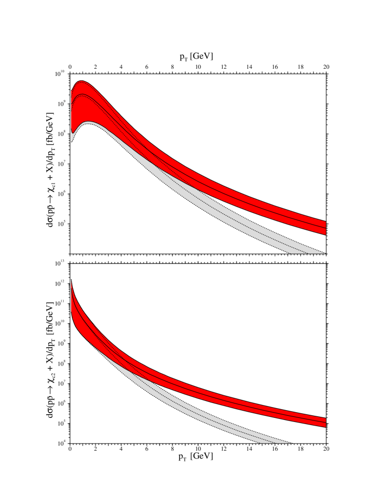
Figure 1: Differential cross sections $d\sigma/dp_{T}$ of $p\overline{p}\to\chi_{cJ}+X$ for $J=1$ (upper frame) and $J=2$ (lower frame) at $\sqrt{S}=1.8$ TeV in NRQCD (solid lines) and the CSM (dashed lines). The central lines represent the default predictions, and the shaded bands indicate the theoretical uncertainties.

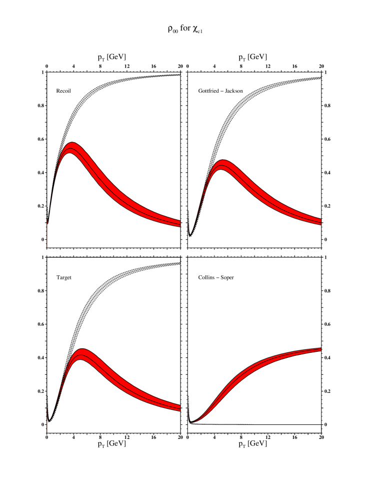
Figure 2: Differential helicity density matrix element $d\rho_{0,0}^{1}/dp_{T}$ of $p\overline{p}\to\chi_{cJ}+X$ at $\sqrt{S}=1.8$ GeV in four different polarization frames in NRQCD (solid lines) and the CSM (dashed lines). The central lines represent the default predictions, and the shaded bands indicate the theoretical uncertainties.

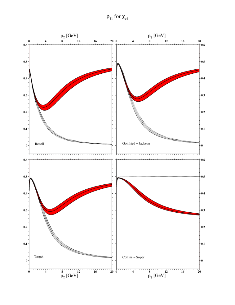
Figure 3: Same as in Fig. 2, but for $d\rho_{1,1}^{1}/dp_{T}$.

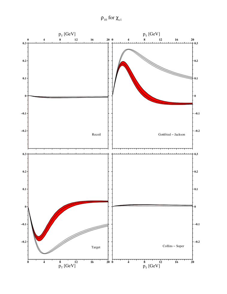
Figure 4: Same as in Fig. 2, but for $d\mathop{\mbox{Re}}\nolimits\rho_{1,0}^{1}/dp_{T}$.

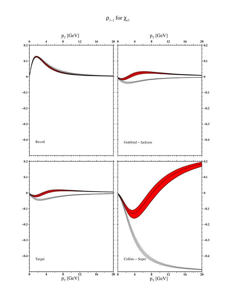
Figure 5: Same as in Fig. 2, but for $d\rho_{1,-1}^{1}/dp_{T}$.

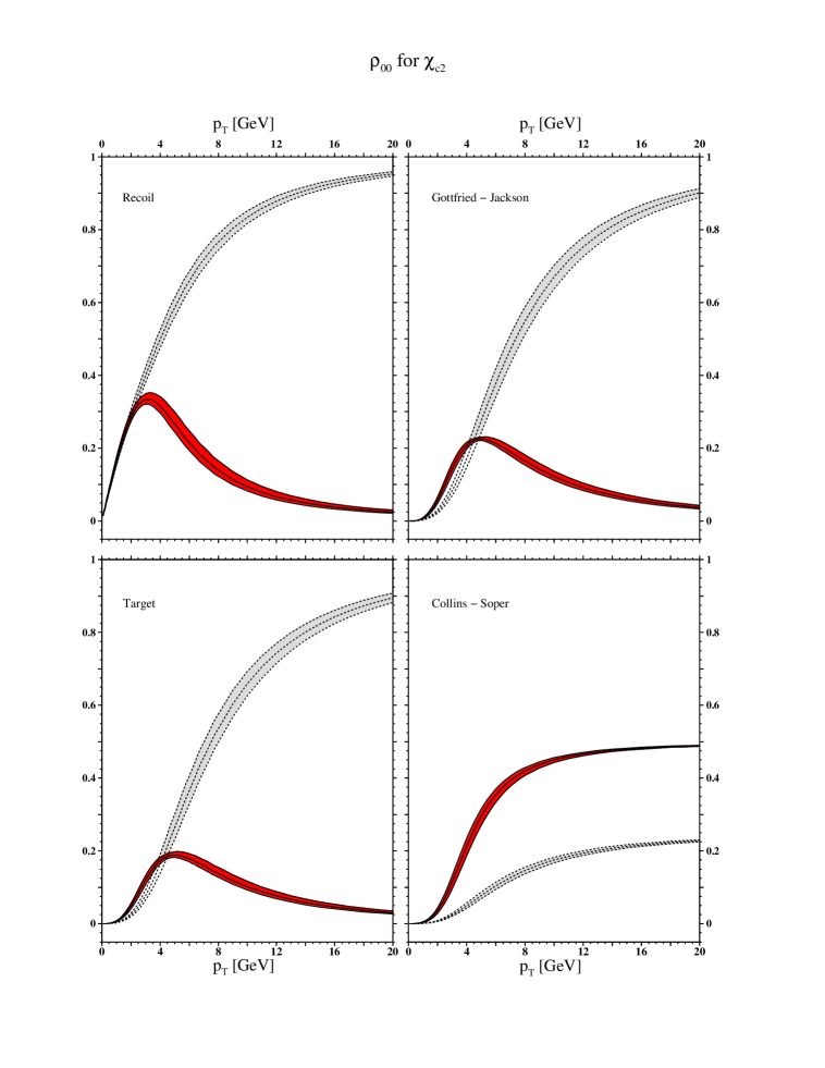
Figure 6: Same as in Fig. 2, but for $d\rho_{0,0}^{2}/dp_{T}$.

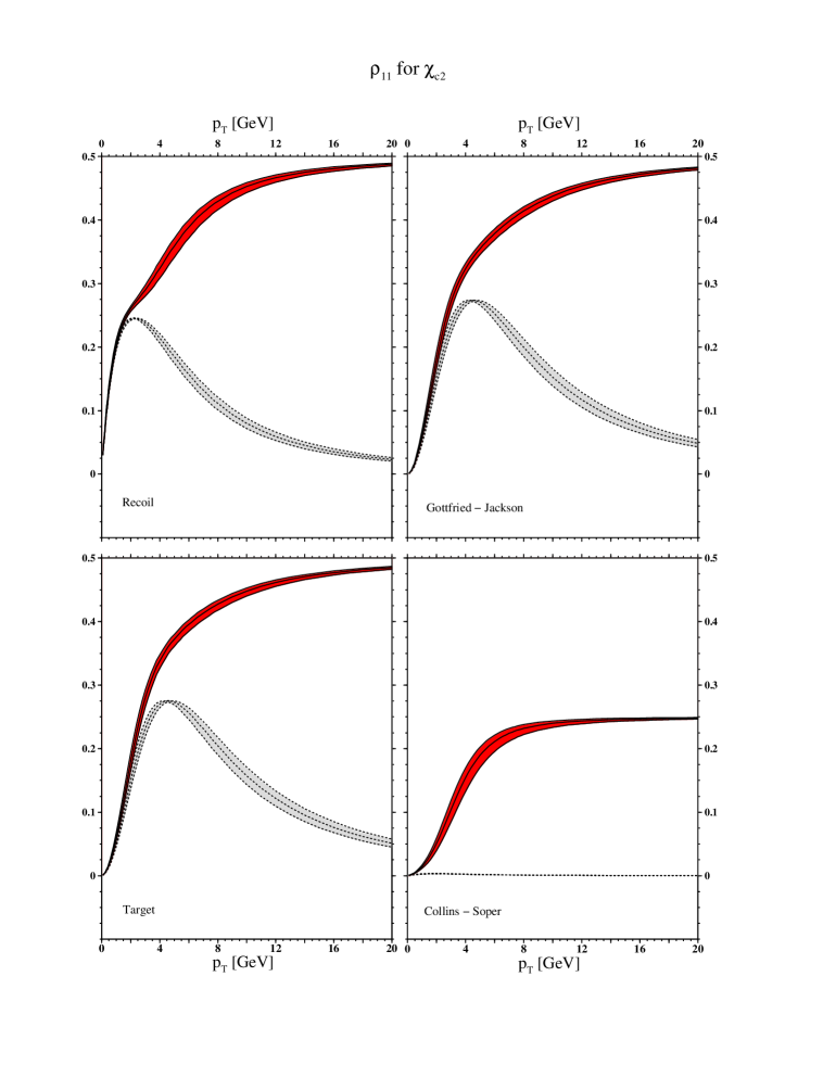
Figure 7: Same as in Fig. 2, but for $d\rho_{1,1}^{2}/dp_{T}$.

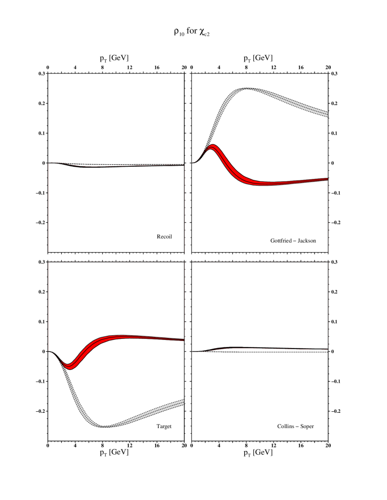
Figure 8: Same as in Fig. 2, but for $d\mathop{\mbox{Re}}\nolimits\rho_{1,0}^{2}/dp_{T}$.

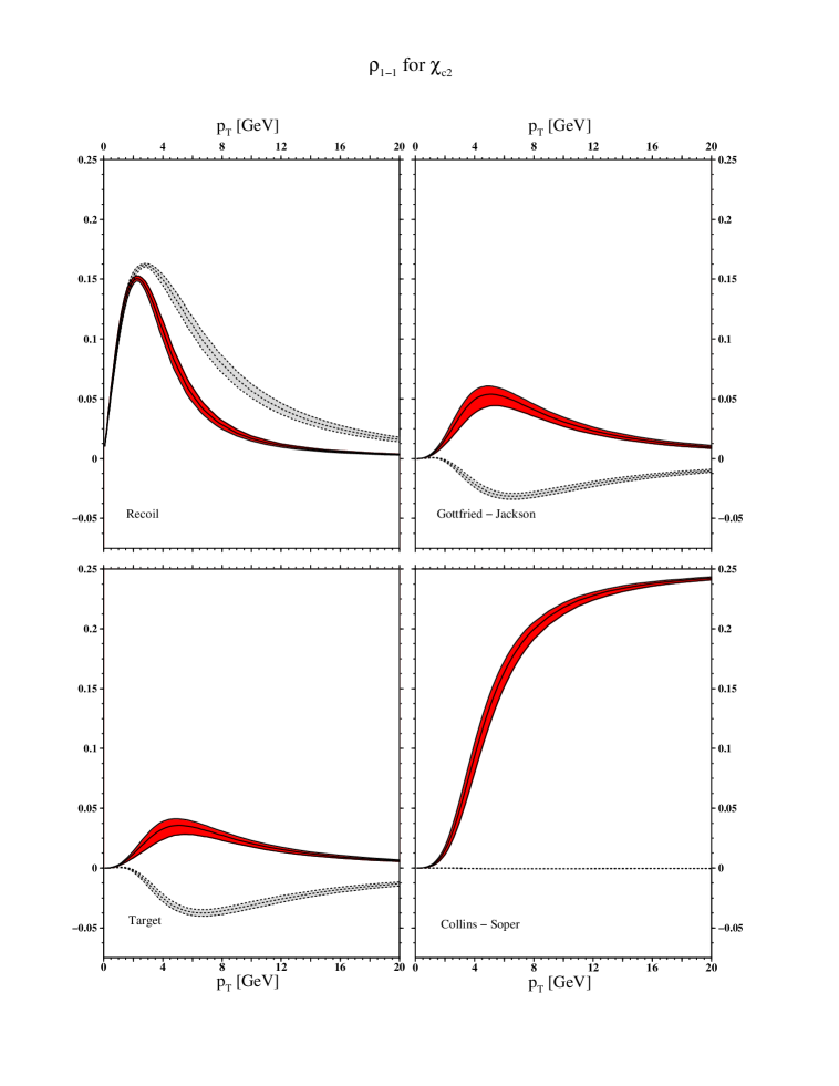
Figure 9: Same as in Fig. 2, but for $d\rho_{1,-1}^{2}/dp_{T}$.

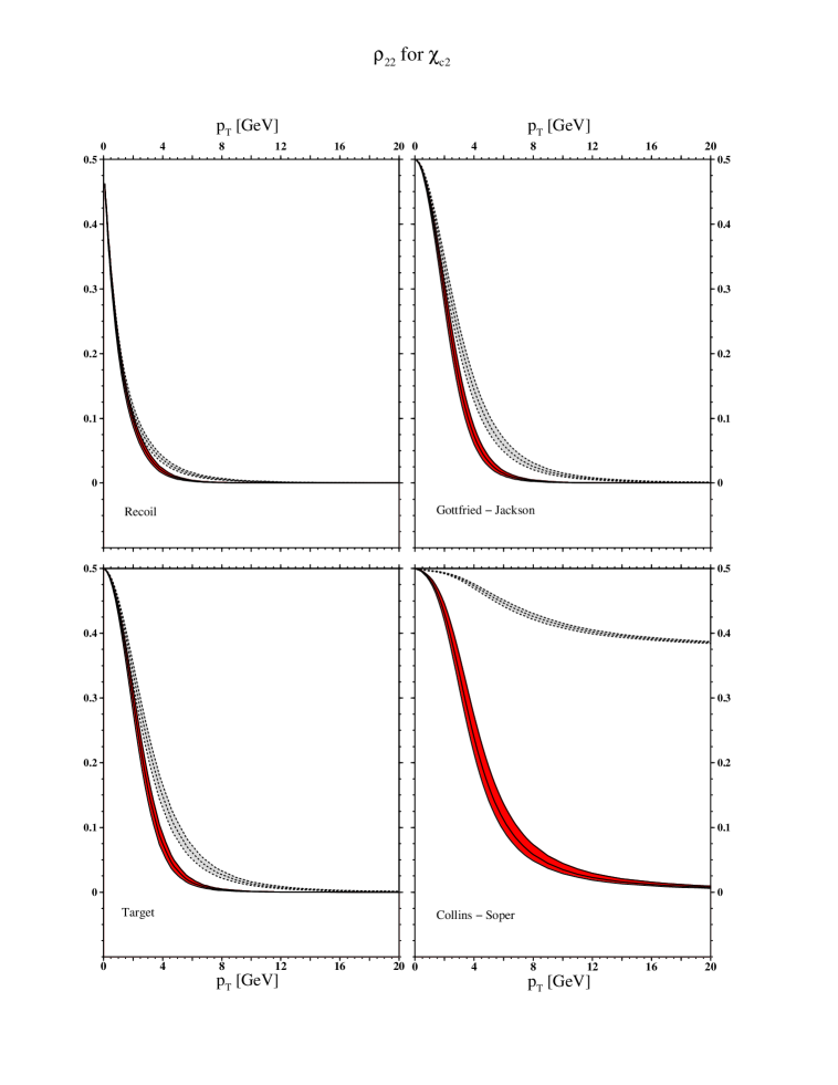
Figure 10: Same as in Fig. 2, but for $d\rho_{2,2}^{2}/dp_{T}$.

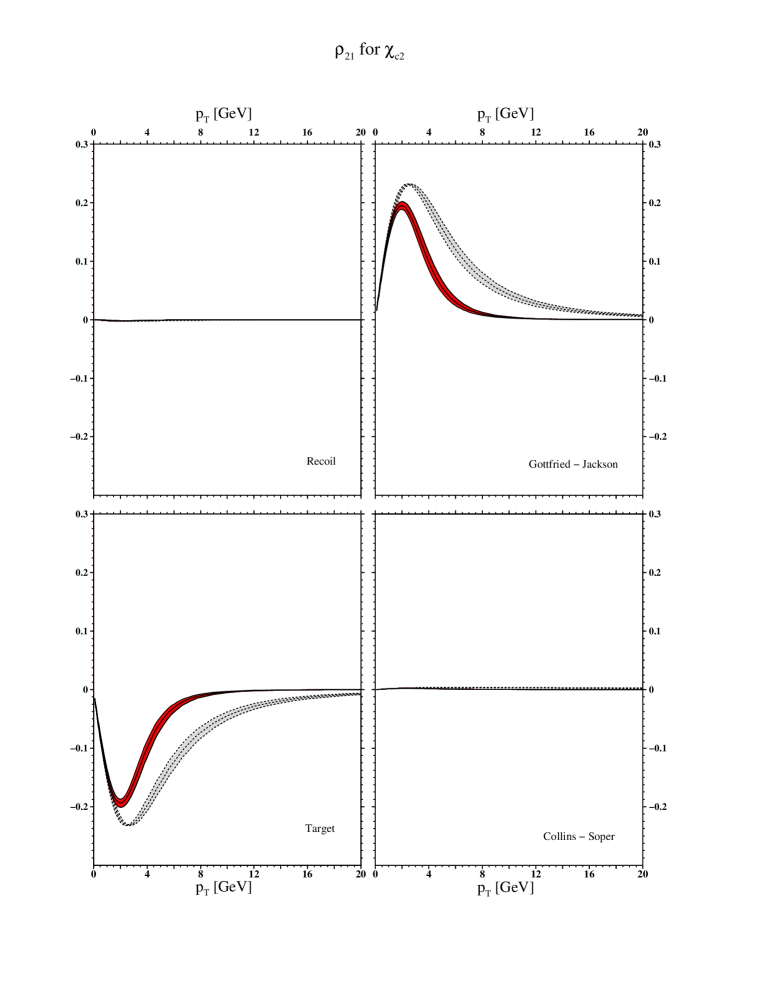
Figure 11: Same as in Fig. 2, but for $d\mathop{\mbox{Re}}\nolimits\rho_{2,1}^{2}/dp_{T}$.

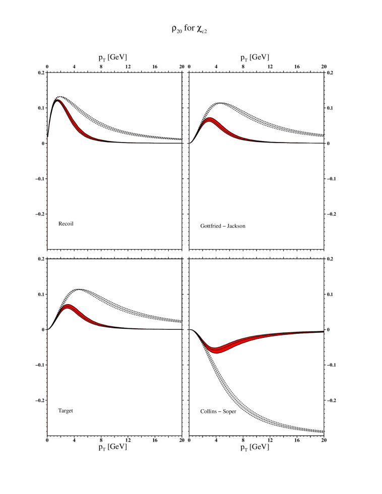
Figure 12: Same as in Fig. 2, but for $d\mathop{\mbox{Re}}\nolimits\rho_{2,0}^{2}/dp_{T}$.

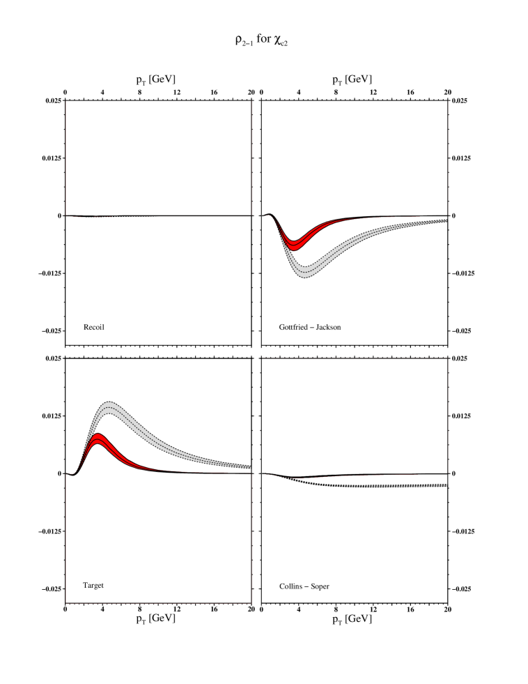
Figure 13: Same as in Fig. 2, but for $d\mathop{\mbox{Re}}\nolimits\rho_{2,-1}^{2}/dp_{T}$.

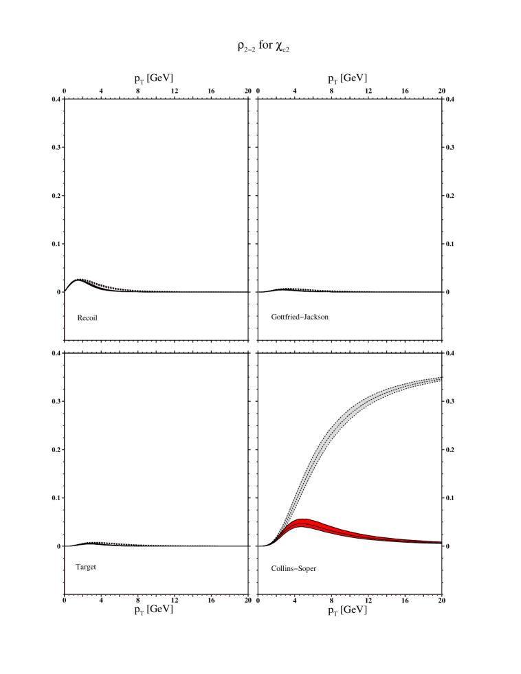
Figure 14: Same as in Fig. 2, but for $d\rho_{2,-2}^{2}/dp_{T}$.