CPsuperH :
a Computational Tool for Higgs Phenomenology
in the Minimal Supersymmetric Standard Model
with Explicit CP Violation

J. S. Lee^a, A. Pilaftsis^a, M. Carena^b, S. Y. Choi^c,
M. Drees^d, J. Ellis^e and C. E. M. Wagner^f,g

^aDepartment of Physics and Astronomy, University of Manchester
Manchester M13 9PL, United Kingdom
^bFermilab, P.O. Box 500, Batavia IL 60510, U.S.A.
^cPhysics Department, Chonbuk National University, Chonju 561–756, Korea
^dPhysik Department, Technische Universität München, D-85748 Garching, Germany
^eTheory Division, CERN, CH-1211 Geneva 23, Switzerland
^fHEP Division, Argonne National Laboratory, 9700 Cass Ave., Argonne, IL 60439, USA
^gEnrico Fermi Institute, Univ. of Chicago, 5640 Ellis Ave., Chicago, IL 60637, USA

ABSTRACT

We provide a detailed description of the Fortran code CPsuperH, a newly–developed computational package that calculates the mass spectrum and decay widths of the neutral and charged Higgs bosons in the Minimal Supersymmetric Standard Model with explicit CP violation. The program is based on recent renormalization-group-improved diagrammatic calculations that include dominant higher–order logarithmic and threshold corrections, $b$-quark Yukawa-coupling resummation effects and Higgs-boson pole-mass shifts. The code CPsuperH is self–contained (with all subroutines included), is easy and fast to run, and is organized to allow further theoretical developments to be easily implemented. The fact that the masses and couplings of the charged and neutral Higgs bosons are computed at a similar high-precision level makes it an attractive tool for Tevatron, LHC and LC studies, also in the CP-conserving case.

1 Introduction

The quest for the still-elusive Higgs boson [1], the missing cornerstone of the renormalizable Standard Model (SM), has become not only more pressing, after the completion of the LEP experimental programme, but also more exciting in light of the upcoming experiments at the upgraded Tevatron collider and the Large Hadron Collider (LHC). Indeed, direct searches for possible realizations of the mechanism of spontaneous electroweak symmetry breaking within and beyond the SM are expected to dominate the scene of particle-physics phenomenology in the present and next decades.

One of the most theoretically appealing realizations of the Higgs mechanism for mass generation is provided by Supersymmetry (SUSY). The minimal supersymmetric extension of the SM (MSSM) has a number of interesting field–theoretic and phenomenological properties, if SUSY is softly broken such that superparticles acquire masses not greatly exceeding 1 TeV. Specifically, within the MSSM, the gauge hierarchy can be made technically natural [2, 3]. Unlike the SM, the MSSM exhibits quantitatively reliable gauge-coupling unification at the energy scale of the order of $10^{16}$ GeV [4]. Furthermore, the MSSM provides a successful mechanism for cosmological baryogenesis via a strongly first-order electroweak phase transition [5, 6], and provides viable candidates for cold dark matter [7, 8].

The MSSM makes a crucial and definite prediction for future high-energy experiments, that can be directly tested at the Tevatron and/or the LHC. It guarantees the existence of (at least) one light neutral Higgs boson with mass less than about 135 GeV [9]. This rather strict upper bound on the lightest Higgs boson mass is in accord with global analyses of the electroweak precision data, which point towards a relatively light SM Higgs boson, with $M_{H_{\rm SM}}\stackrel{{\scriptstyle<}}{{{}_{\sim}}}211$ GeV at the 95 % confidence level [10]. Furthermore, because of the decoupling properties of heavy superpartners, the MSSM predictions for the electroweak precision observables can easily be made consistent with all the experimental data [11].

Recently, a new important phenomenological feature of the MSSM Higgs sector has been observed. It has been realized that loop effects mediated dominantly by third-generation squarks may lead to sizeable violations of the tree-level CP invariance of the MSSM Higgs potential, giving rise to significant Higgs scalar-pseudoscalar transitions [12], in particular. As a consequence, the three neutral Higgs mass eigenstates $H_{1,2,3}$, labelled in order of increasing mass such that $M_{H_{1}}\leq M_{H_{2}}\leq M_{H_{3}}$, have no definite CP parities, but become mixtures of CP-even and CP-odd states. Much work has been devoted to studying in greater detail this radiative Higgs–sector CP violation in the framework of the MSSM [13, 14, 15, 16, 17, 18, 19, 20, 21, 23, 22]. In the MSSM with explicit CP violation, the couplings of the Higgs bosons to the SM gauge bosons and fermions, to their supersymmetric partners and to the Higgs bosons themselves may be considerably modified from those predicted in the CP-conserving case. Consequently, radiative CP violation in the MSSM Higgs sector can significantly affect the production rates and decay branching fractions of the Higgs bosons. In particular, the drastic modification of the couplings of the $Z$ boson to the two lighter Higgs bosons $H_{1}$ and $H_{2}$ might enable a relatively light Higgs boson with a mass $M_{H_{1}}$ even less than about 70 GeV to have escaped detection at LEP 2 [16, 22]. The upgraded Tevatron collider and the LHC will be able to cover a large fraction of the MSSM parameter space, including the challenging regions with a light Higgs boson without definite CP parity [24, 22, 25]. Furthermore, complementary and more accurate explorations of the CP-noninvariant MSSM Higgs sector can be carried out using high-luminosity $e^{+}e^{-}$ [26] and/or $\gamma\gamma$ [27] colliders. In addition, a complete determination of the CP properties of the neutral Higgs bosons is possible at muon colliders by exploiting polarized muon beams [28].

It is obvious that a systematic study of Higgs phenomenology in the MSSM with explicit CP violation would be greatly facilitated by an appropriate computational tool. For this purpose, we have developed the Fortran program CPsuperH, a new self–contained computational package, which calculates the mass spectrum and the decay widths of the neutral and charged Higgs bosons in the MSSM with explicit CP violation. It calculates the neutral Higgs-boson masses $M_{H_{1,2,3}}$ and the corresponding $3\times 3$ Higgs-boson mixing matrix $O$, employing the renormalization-group- (RG-)improved diagrammatic approach of [23]. We include the leading two-loop QCD logarithmic corrections as well as the leading two-loop logarithmic corrections induced by the top- and bottom-quark Yukawa couplings [30]. We also include the leading one-loop logarithmic corrections due to gaugino and higgsino quantum effects [31]. Moreover, we implement the potentially large two–loop non–logarithmic corrections originating from one–loop threshold effects on the top- and bottom-quark Yukawa couplings, associated with the decoupling of the third-generation squarks [32, 16, 15]. Finally, the RG-improved diagrammatic calculation takes account of mass shifts determined by the positions of the poles in the corresponding Higgs-boson propagators. These Higgs–boson pole-mass shifts for the lightest Higgs boson are small, of the order of a few GeV. However, the mass shifts for the heavier Higgs bosons, $H_{2}$ and $H_{3}$, can be much larger and of the order of several tens of GeV [23], especially if their masses $M_{H_{2}}$ and $M_{H_{3}}$ happen to be close to thresholds for the on-shell production of squark pairs. Finally, we note that the computation of all the Higgs-boson decay widths by the code CPsuperH relies on the extensive analytic results for the decay widths presented in [18].

After this introductory discussion, the next section summarizes all the topics of Higgs phenomenology that can be studied with the code CPsuperH. In Section 3, we describe the execution procedure of the Fortran code and present examples of input and output files from a test run. Finally, we summarize the essential features of the code and provide an outlook for further developments of CPsuperH in Section 4.

2 Higgs Phenomenology in the MSSM with Explicit
CP Violation

In the presence of nontrivial CP–violating phases for the higgsino mass parameter $\mu$ and the soft SUSY–breaking parameters in the MSSM, the couplings of the Higgs bosons to the gauge bosons, fermions and sfermions, as well as those to the Higgs bosons themselves, are strongly modified. In order to investigate these modifications and their phenomenological implications, we begin by stating our conventions for the mixing matrices of the neutral Higgs bosons and SUSY particles, and then we present all the relevant Higgs interactions with the MSSM particles to be used subsequently for calculating the masses, total decay widths and decay branching fractions of the neutral and charged Higgs bosons.

2.1 Conventions

In this subsection, we give our conventions for the mixing matrices of neutral Higgs bosons, charginos, neutralinos and third–generation sfermions.

• Neutral Higgs bosons: In the presence of nontrivial CP-violating phases of the soft supersymmetry-breaking parameters, most relevantly in the third-generation sfermion sector, the three neutral Higgs bosons all mix together via radiative corrections:

  $$(\phi_{1},\phi_{2},a)^{T}_{\alpha}=O_{\alpha i}(H_{1},H_{2},H_{3})^{T}_{i}\,,$$ (1)

  where $O^{T}{\cal M}^{2}_{H}\,O={\sf diag}\,(M^{2}_{H_{1}},M^{2}_{H_{2}},M^{2}_{H_{3}})$ with $M_{H_{1}}\leq M_{H_{2}}\leq M_{H_{3}}$. We refer to [16, 23] for the details of the calculations of the mass-squared matrix ${\cal M}^{2}_{H}$, the diagonalization matrix $O$ and the pole masses of the Higgs bosons.

• Charginos: In SUSY theories, the spin–1/2 partners of the $W^{\pm}$ gauge bosons and the charged Higgs bosons, $\tilde{W}^{\pm}$ and $\tilde{H}^{\pm}$, mix to form chargino mass eigenstates. We adopt the convention $\tilde{H}^{-}_{L(R)}=\tilde{H}^{-}_{1(2)}$, where the subscripts 1 and 2 are associated with the Higgs supermultiplets leading to the tree-level mass generation of the down- and up-type quarks, respectively. The chargino mass matrix in the $(\tilde{W}^{-},\tilde{H}^{-})$ basis

  $${\cal M}_{C}=\left(\begin{array}[]{cc}M_{2}&\sqrt{2}M_{W}\,c_{\beta}\\[5.69054pt] \sqrt{2}M_{W}\,s_{\beta}&\mu\end{array}\right)\,,$$ (4)

  is diagonalized by two different unitary matrices $C_{R}{\cal M}_{C}C_{L}^{\dagger}={\sf diag}\{m_{\tilde{\chi}^{\pm}_{1}},\,m_{\tilde{\chi}^{\pm}_{2}}\}$, where $m_{\tilde{\chi}^{\pm}_{1}}\leq m_{\tilde{\chi}^{\pm}_{2}}$. The chargino mixing matrices $(C_{L})_{i\alpha}$ and $(C_{R})_{i\alpha}$ relate the electroweak eigenstates to the mass eigenstates, via

  $$\tilde{\chi}^{-}_{\alpha L} = (C_{L})^{*}_{i\alpha}\tilde{\chi}_{iL}^{-}\,,\qquad\tilde{\chi}^{-}_{\alpha L}\ =\ (\tilde{W}^{-},\tilde{H}^{-})_{L}^{T}\,,$$

  $$\tilde{\chi}^{-}_{\alpha R} = (C_{R})^{*}_{i\alpha}\tilde{\chi}_{iR}^{-}\,,\qquad\tilde{\chi}^{-}_{\alpha R}\ =\ (\tilde{W}^{-},\tilde{H}^{-})_{R}^{T}\,.$$ (5)

  We use the following abbreviations throughout this paper: $s_{\beta}\equiv\sin\beta$, $c_{\beta}\equiv\cos\beta$, $t_{\beta}=\tan\beta$, $s_{2\beta}\equiv\sin\,2\beta$, $c_{2\beta}\equiv\cos\,2\beta$, $s_{W}\equiv\sin\theta_{W}$, $c_{W}\equiv\cos\theta_{W}$, etc.

• Neutralinos: The neutralino mass matrix in the $(\tilde{B},\tilde{W}^{3},\tilde{H}^{0}_{1},\tilde{H}^{0}_{2})$ basis is given by

  $${\cal M}_{N}=\left(\begin{array}[]{cccc}M_{1}&0&-M_{Z}c_{\beta}s_{W}&M_{Z}s_{\beta}s_{W}\\[5.69054pt] 0&M_{2}&M_{Z}c_{\beta}c_{W}&-M_{Z}s_{\beta}c_{W}\\[5.69054pt] -M_{Z}c_{\beta}s_{W}&M_{Z}c_{\beta}c_{W}&0&-\mu\\[5.69054pt] M_{Z}s_{\beta}s_{W}&-M_{Z}s_{\beta}c_{W}&-\mu&0\end{array}\right)\,.$$ (10)

  This neutralino mass matrix is diagonalized by a unitary matrix $N$: $N^{*}{\cal M}_{N}N^{\dagger}={\sf diag}\,(m_{\tilde{\chi}_{1}^{0}},m_{\tilde{\chi}_{2}^{0}},m_{\tilde{\chi}_{3}^{0}},m_{\tilde{\chi}_{4}^{0}})$ with $m_{\tilde{\chi}_{1}^{0}}\leq m_{\tilde{\chi}_{2}^{0}}\leq m_{\tilde{\chi}_{3}^{0}}\leq m_{\tilde{\chi}_{4}^{0}}$. The neutralino mixing matrix $N_{i\alpha}$ relates the electroweak eigenstates to the mass eigenstates via

  $$(\tilde{B},\tilde{W}^{3},\tilde{H}^{0}_{1},\tilde{H}^{0}_{2})^{T}_{\alpha}=N_{i\alpha}^{*}({\tilde{\chi}_{1}^{0}},{\tilde{\chi}_{2}^{0}},{\tilde{\chi}_{3}^{0}},{\tilde{\chi}_{4}^{0}})^{T}_{i}\,.$$ (11)

• Stops, sbottoms, staus and tau sneutrino: The stop and sbottom mass matrices may conveniently be written in the $\left(\tilde{q}_{L},\tilde{q}_{R}\right)$ basis as

  $$\widetilde{\cal M}^{2}_{q}=\left(\begin{array}[]{cc}M^{2}_{\tilde{Q}_{3}}\,+\,m^{2}_{q}\,+\,c_{2\beta}M^{2}_{Z}\,(T^{q}_{z}\,-\,Q_{q}s_{W}^{2})&h_{q}^{*}v_{q}(A^{*}_{q}-\mu R_{q})/\sqrt{2}\\ h_{q}v_{q}(A_{q}-\mu^{*}R_{q})/\sqrt{2}&M^{2}_{\tilde{R}_{3}}\,+\,m^{2}_{q}\,+\,c_{2\beta}M^{2}_{Z}\,Q_{q}s^{2}_{W}\end{array}\right)\,,$$ (12)

  with $q=t,b$, $R=U,D$, $T^{t}_{z}=-T^{b}_{z}=1/2$, $Q_{t}=2/3$, $Q_{b}=-1/3$, $v_{b}=v_{1}$, $v_{t}=v_{2}$, $R_{b}=\tan\beta=v_{2}/v_{1}$, $R_{t}=\cot\beta$, and $h_{q}$ is the Yukawa coupling of the quark $q$. On the other hand, the stau mass matrix is written in the $\left(\tilde{\tau}_{L},\tilde{\tau}_{R}\right)$ basis as

  $$\widetilde{\cal M}^{2}_{\tau}=\left(\begin{array}[]{cc}M^{2}_{\tilde{L}_{3}}\,+\,m^{2}_{\tau}\,+\,c_{2\beta}M^{2}_{Z}\,(s_{W}^{2}-1/2)&h_{\tau}^{*}v_{1}(A^{*}_{\tau}-\mu\tan\beta)/\sqrt{2}\\ h_{\tau}v_{1}(A_{\tau}-\mu^{*}\tan\beta)/\sqrt{2}&M^{2}_{\tilde{E}_{3}}\,+\,m^{2}_{\tau}\,-\,c_{2\beta}M^{2}_{Z}\,s^{2}_{W}\end{array}\right)\,,$$ (15)

  and the mass of the tau sneutrino $\tilde{\nu_{\tau}}$ is simply $m_{\tilde{\nu}_{\tau}}=\sqrt{M^{2}_{\tilde{L}_{3}}+\frac{1}{2}c_{2\beta}M_{Z}^{2}}$, as it has no right–handed counterpart in the MSSM. The $2\times 2$ sfermion mass matrix $\widetilde{\cal M}^{2}_{f}$ for $f=t,b$ and $\tau$ is diagonalized by a unitary matrix $U^{\tilde{f}}$: $U^{\tilde{f}\dagger}\,\widetilde{\cal M}^{2}_{f}\,U^{\tilde{f}}={\sf diag}(m_{\tilde{f}_{1}}^{2},m_{\tilde{f}_{2}}^{2})\,$ with $m_{\tilde{f}_{1}}^{2}\leq m_{\tilde{f}_{2}}^{2}$. The mixing matrix $U^{\tilde{f}}$ relates the electroweak eigenstates $\tilde{f}_{L,R}$ to the mass eigenstates $\tilde{f}_{1,2}$, via

  $$(\tilde{f}_{L},\tilde{f}_{R})^{T}_{\alpha}\,=\,U^{\tilde{f}}_{\alpha i}\,(\tilde{f}_{1},\tilde{f}_{2})^{T}_{i}\,.$$ (16)

  We parameterize the mixing matrices as follows:

  $$U^{\tilde{f}}=\left(\begin{array}[]{cc}\cos\theta_{\tilde{f}}&-\sin\theta_{\tilde{f}}\,{\rm e}^{-i\phi_{\tilde{f}}}\\ \sin\theta_{\tilde{f}}\,{\rm e}^{+i\phi_{\tilde{f}}}&\cos\theta_{\tilde{f}}\end{array}\right)\,,$$ (19)

  and we calculate numerically the mixing angle $\theta_{\tilde{f}}$ and phase $\phi_{\tilde{f}}$ in the ranges between $-\pi/2$ and $\pi/2$, so that $\cos\theta_{\tilde{f}}\geq 0$ and $\cos\phi_{\tilde{f}}\geq 0$.

2.2 Higgs–Boson Interactions

In this subsection, we list all the Higgs interactions with gauge bosons, SM fermions, squarks, sleptons, charginos, and neutralinos. We also present all the trilinear and quartic Higgs–boson self–couplings.

• Interactions of Higgs bosons with gauge bosons: The interactions of the Higgs bosons with the gauge bosons $Z$ and $W^{\pm}$ are described by the three interaction Lagrangians:

  $${\cal L}_{HVV} = g\,M_{W}\,\left(W^{+}_{\mu}W^{-\mu}\ +\ \frac{1}{2c_{W}^{2}}\,Z_{\mu}Z^{\mu}\right)\,\sum_{i}\,g_{{}_{H_{i}VV}}\,H_{i}\,,$$ (20)

  $${\cal L}_{HHZ} = \frac{g}{4c_{W}}\sum_{i,j}g_{{}_{H_{i}H_{j}Z}}\,Z^{\mu}(H_{i}\,i\!\stackrel{{\scriptstyle\leftrightarrow}}{{\partial}}_{\mu}H_{j})\,,$$ (21)

  $${\cal L}_{HH^{\pm}W^{\mp}} = -\frac{g}{2}\,\sum_{i}\,g_{{}_{H_{i}H^{+}W^{-}}}\,W^{-\mu}(H_{i}\,i\!\stackrel{{\scriptstyle\leftrightarrow}}{{\partial}}_{\mu}H^{+})\,+\,{\rm h.c.}\,,$$ (22)

  where $g=e/\sin\theta_{W}$ is the SU(2)_L gauge-coupling constant, and the couplings $g_{{}_{H_{i}VV}}$, $g_{{}_{H_{i}H_{j}Z}}$ and $g_{{}_{H_{i}H^{+}W^{-}}}$ are given in terms of the neutral Higgs-boson mixing matrix $O$ by (note that det$(O)=\pm 1$ for any orthogonal matrix $O$):

  $$g_{{}_{H_{i}VV}} = c_{\beta}\,O_{\phi_{1}i}\>+\>s_{\beta}\,O_{\phi_{2}i}\,,$$

  $$g_{{}_{H_{i}H_{j}Z}} = {\rm sign}[{\rm det}(O)]\,\,\varepsilon_{ijk}\,g_{{}_{H_{k}VV}}\,,$$

  $$g_{{}_{H_{i}H^{+}W^{-}}} = c_{\beta}\,O_{\phi_{2}i}-s_{\beta}\,O_{\phi_{1}i}-iO_{ai}\,,$$ (23)

  leading to the following sum rules:

  $$\sum_{i=1}^{3}\,g_{{}_{H_{i}VV}}^{2}\ =\ 1\,\quad{\rm and}\quad g_{{}_{H_{i}VV}}^{2}+|g_{{}_{H_{i}H^{+}W^{-}}}|^{2}\ =\ 1\,\quad{\rm for~{}each}~{}i\,.$$ (24)

• Higgs–quark–antiquark and Higgs–lepton-antilepton interactions: The effective Lagrangian governing the interactions of the neutral Higgs bosons with quarks and charged leptons is

  $${\cal L}_{H_{i}\bar{f}f}\ =\ -\sum_{f=u,d,l}\,\frac{gm_{f}}{2M_{W}}\,\sum_{i=1}^{3}\,H_{i}\,\bar{f}\,\Big{(}g^{S}_{H_{i}\bar{f}f}\,+\,ig^{P}_{H_{i}\bar{f}f}\gamma_{5}\Big{)}\,f\ .$$ (25)

  At the tree level, $(g^{S},g^{P})=(O_{\phi_{1}i}/c_{\beta},-O_{ai}\tan\beta)$ and $(g^{S},g^{P})=(O_{\phi_{2}i}/s_{\beta},-O_{ai}\cot\beta)$ for $f=(l,d)$ and $f=u$, respectively. In the case of third-generation quarks, the program CPsuperH computes the finite threshold corrections induced by the exchanges of gluinos and charginos. As described in Appendix A, we include the all–orders resummation [33, 34, 22] of the leading powers of $\tan\beta$, as required for a meaningful perturbative expansion. Correspondingly, in the presence of CP violation, the effective couplings of the charged Higgs boson to quarks and leptons in the weak-interaction basis are described by the interaction Lagrangian:

  $${\cal L}_{H^{\pm}f_{\uparrow}f_{\downarrow}}\ =\ \frac{g}{\sqrt{2}M_{W}}\,\hskip-5.69046pt\sum_{(f_{\uparrow},f_{\downarrow})=(u,d),(\nu,l)}\hskip-8.5359ptH^{+}\,\bar{f}_{\uparrow}\,\Big{(}\,m_{f_{\uparrow}}\,g^{L}_{H^{+}\bar{f}_{\uparrow}f_{\downarrow}}\,P_{L}\ +\ m_{f_{\downarrow}}\,g^{R}_{H^{+}\bar{f}_{\uparrow}f_{\downarrow}}\,P_{R}\,\Big{)}\,f_{\downarrow}\ +\ {\rm h.c.},$$ (26)

  where $P_{L/R}\equiv(1\,\mp\,\gamma_{5})/2$. At the tree level, $g^{L}=\cot\beta$ and $g^{R}=\tan\beta$ with $m_{\nu}=0$. The loop–induced threshold corrections to the $g^{L,R}_{H^{+}\bar{u}d}$ couplings are presented in Appendix A.

• Higgs–sfermion–sfermion interactions: The Higgs–sfermion–sfermion interactions can be written in terms of the sfermion mass eigenstates as

  $${\cal L}_{H\tilde{f}\tilde{f}}=v\sum_{f=u,d}\,g_{H_{i}\tilde{f}^{*}_{j}\tilde{f}_{k}}(H_{i}\,\tilde{f}^{*}_{j}\,\tilde{f}_{k})\,,$$ (27)

  where

  $$v\,g_{H_{i}\tilde{f}^{*}_{j}\tilde{f}_{k}}=\left(\Gamma^{\alpha\tilde{f}^{*}\tilde{f}}\right)_{\beta\gamma}O_{\alpha i}U^{\tilde{f}*}_{\beta j}U^{\tilde{f}}_{\gamma k}\,,$$

  with $\alpha=(\phi_{1},\phi_{2},a)=(1,2,3)$, $\beta,\gamma=L,R$, $i=(H_{1},H_{2},H_{3})=(1,2,3)$ and $j,k=1,2$. Likewise, the charged Higgs-boson interactions with up– and down–type sfermions are given by

  $${\cal L}_{H^{\pm}\tilde{f}\tilde{f^{\prime}}}=v\,g_{H^{+}\tilde{f}^{*}_{j}\tilde{f^{\prime}}_{k}}(H^{+}\,\tilde{f}^{*}_{j}\,\tilde{f^{\prime}}_{k})+{\rm h.c.},$$ (28)

  where

  $$v\,g_{H^{+}\tilde{f}^{*}_{j}\tilde{f^{\prime}}_{k}}\ =\ \left(\Gamma^{H^{+}\tilde{f}^{*}\tilde{f^{\prime}}}\right)_{\beta\gamma}\,U^{\tilde{f}*}_{\beta j}\,U^{\tilde{f^{\prime}}}_{\gamma k}\,.$$

  The expressions for the couplings $\Gamma^{\alpha\tilde{f}^{*}\tilde{f}}$ and $\Gamma^{H^{+}\tilde{f}^{*}\tilde{f^{\prime}}}$ to third–generation sfermions are presented in Appendix B. As shown in [34], our iterative treatment of the threshold corrections that are enhanced at large $\tan\beta$ ensures that the corresponding corrections to the Higgs-boson couplings to squarks are also resummed correspondingly.

• Interactions of neutral Higgs bosons and charginos: These are described by the following Lagrangian:

  $${\cal L}_{H^{0}\widetilde{\chi}^{+}\widetilde{\chi}^{-}} = -\frac{g}{\sqrt{2}}\sum_{i,j,k}H_{k}\overline{\widetilde{\chi}_{i}^{-}}\left(g_{H_{k}\tilde{\chi}^{+}_{i}\tilde{\chi}^{-}_{j}}^{S}+i\gamma_{5}g_{H_{k}\tilde{\chi}^{+}_{i}\tilde{\chi}^{-}_{j}}^{P}\right)\widetilde{\chi}_{j}^{-}\,,$$

  $$g_{H_{k}\tilde{\chi}^{+}_{i}\tilde{\chi}^{-}_{j}}^{S} = \frac{1}{2}\left\{[(C_{R})_{i1}(C_{L})^{*}_{j2}G^{\phi_{1}}_{k}+(C_{R})_{i2}(C_{L})^{*}_{j1}G^{\phi_{2}}_{k}]+[i\leftrightarrow j]^{*}\right\}\,,$$

  $$g_{H_{k}\tilde{\chi}^{+}_{i}\tilde{\chi}^{-}_{j}}^{P} = \frac{i}{2}\left\{[(C_{R})_{i1}(C_{L})^{*}_{j2}G^{\phi_{1}}_{k}+(C_{R})_{i2}(C_{L})^{*}_{j1}G^{\phi_{2}}_{k}]-[i\leftrightarrow j]^{*}\right\}\,,$$ (29)

  where $G^{\phi_{1}}_{k}=(O_{\phi_{1}k}-is_{\beta}O_{ak})$, $G^{\phi_{2}}_{k}=(O_{\phi_{2}k}-ic_{\beta}O_{ak})$, $i,j=1,2$, and $k=1-3$.

• Interactions of neutral Higgs bosons and neutralinos: These are described by the following Lagrangian:

  $${\cal L}_{H^{0}\widetilde{\chi}^{0}\widetilde{\chi}^{0}} = -\frac{g}{2}\sum_{i,j,k}H_{k}\overline{\widetilde{\chi}_{i}^{0}}\left(g_{H_{k}\tilde{\chi}^{0}_{i}\tilde{\chi}^{0}_{j}}^{S}+i\gamma_{5}g_{H_{k}\tilde{\chi}^{0}_{i}\tilde{\chi}^{0}_{j}}^{P}\right)\widetilde{\chi}_{j}^{0}\,:$$

  $$g_{H_{k}\tilde{\chi}^{0}_{i}\tilde{\chi}^{0}_{j}}^{S} = \frac{1}{2}\Re{\rm e}{[(N_{j2}^{*}-t_{W}N_{j1}^{*})(N_{i3}^{*}G^{\phi_{1}}_{k}-N_{i4}^{*}G^{\phi_{2}}_{k})+(i\leftrightarrow j)]}$$

  $$g_{H_{k}\tilde{\chi}^{0}_{i}\tilde{\chi}^{0}_{j}}^{P} = -\frac{1}{2}\Im{\rm m}{[(N_{j2}^{*}-t_{W}N_{j1}^{*})(N_{i3}^{*}G^{\phi_{1}}_{k}-N_{i4}^{*}G^{\phi_{2}}_{k})+(i\leftrightarrow j)]}\,,$$ (30)

  where $i,j=1$-$4$ for the four neutralino states and $k=1$-$3$ for the three neutral Higgs bosons.

• Interactions of charged Higgs bosons, charginos and neutralinos: These are described by the following Lagrangian:

  $${\cal L}_{H^{\pm}\widetilde{\chi}_{i}^{0}\widetilde{\chi}_{j}^{\mp}} = -\frac{g}{\sqrt{2}}\sum_{i,j}H^{+}\,\overline{\widetilde{\chi}_{i}^{0}}\left(g_{H^{+}\tilde{\chi}^{0}_{i}\tilde{\chi}^{-}_{j}}^{S}+i\gamma_{5}g_{H^{+}\tilde{\chi}^{0}_{i}\tilde{\chi}^{-}_{j}}^{P}\right)\widetilde{\chi}_{j}^{-}+{\rm h.c.}\,:$$

  $$g_{H^{+}\tilde{\chi}^{0}_{i}\tilde{\chi}^{-}_{j}}^{S} = \frac{1}{2}\left\{s_{\beta}\left[\sqrt{2}N_{i3}^{*}(C_{L})_{j1}^{*}-(N_{i2}^{*}+t_{W}N_{i1}^{*})(C_{L})_{j2}^{*}\right]\right.$$

  $$\left.~{}+c_{\beta}\left[\sqrt{2}N_{i4}(C_{R})_{j1}^{*}+(N_{i2}+t_{W}N_{i1})(C_{R})_{j2}^{*}\right]\right\}\,,$$

  $$g_{H^{+}\tilde{\chi}^{0}_{i}\tilde{\chi}^{-}_{j}}^{P} = \frac{i}{2}\left\{s_{\beta}\left[\sqrt{2}N_{i3}^{*}(C_{L})_{j1}^{*}-(N_{i2}^{*}+t_{W}N_{i1}^{*})(C_{L})_{j2}^{*}\right]\right.$$ (31)

  $$\left.~{}-c_{\beta}\left[\sqrt{2}N_{i4}(C_{R})_{j1}^{*}+(N_{i2}+t_{W}N_{i1})(C_{R})_{j2}^{*}\right]\right\}\,.$$

• Trilinear and quartic Higgs-boson self-couplings  [18, 22]: The effective trilinear and quartic Higgs self–couplings can be cast into the form

  $${\cal L}_{3H} = v\,\sum_{i\geq j\geq k=1}^{3}g_{{}_{H_{i}H_{j}H_{k}}}\,H_{i}H_{j}H_{k}\>+\>v\,\sum_{i=1}^{3}g_{{}_{H_{i}H^{+}H^{-}}}\,H_{i}H^{+}H^{-}\,,$$ (32)

  $${\cal L}_{4H} = \sum_{i\geq j\geq k\geq l=1}^{3}g_{{}_{H_{i}H_{j}H_{k}H_{l}}}\,H_{i}H_{j}H_{k}H_{l}\ +\ \sum_{i\geq j=1}^{3}g_{{}_{H_{i}H_{j}H^{+}H^{-}}}\,H_{i}H_{j}H^{+}H^{-}$$ (33)

  $$+\ g_{{}_{H^{+}H^{-}H^{+}H^{-}}}\,(H^{+}H^{-})^{2}\,,\$$

  where

  $$g_{{}_{H_{i}H_{j}H_{k}}} = \sum_{\alpha\leq\beta\leq\gamma=1}^{3}\left\{O_{\alpha i}O_{\beta j}O_{\gamma k}\right\}\,g_{\alpha\beta\gamma}\,,\quad g_{{}_{H_{i}H^{+}H^{-}}}\ =\ \sum_{\alpha=1}^{3}O_{\alpha i}\,g_{{}_{\alpha H^{+}H^{-}}}\,,\quad$$ (34)

  $$g_{{}_{H_{i}H_{j}H_{k}H_{l}}} = \sum_{\alpha\leq\beta\leq\gamma\leq\delta=1}^{3}\left\{O_{\alpha i}O_{\beta j}O_{\gamma k}O_{\delta l}\right\}\,g_{\alpha\beta\gamma\delta}\,,$$

  $$g_{{}_{H_{i}H_{j}H^{+}H^{-}}} = \sum_{\alpha\leq\beta=1}^{3}\left\{O_{\alpha i}O_{\beta j}\right\}\,g_{\alpha\beta{\scriptscriptstyle H^{+}H^{-}}}\,.$$ (35)

  In the above equations (34) and (35), the expressions within the curly brackets $\{\cdots\}$ need to be symmetrized with respect to the indices $i,j,k,l$ and divided by the corresponding symmetry factors in cases where two or more indices are the same. For example, $\left\{O_{\alpha i}O_{\beta j}O_{\gamma k}\right\}$ can explicitly be evaluated as follows:

  $$\left\{O_{\alpha i}O_{\beta j}O_{\gamma k}\right\} \equiv \frac{1}{N_{S}}\,\Big{(}O_{\alpha i}O_{\beta j}O_{\gamma k}+O_{\alpha i}O_{\beta k}O_{\gamma j}+O_{\alpha j}O_{\beta i}O_{\gamma k}+O_{\alpha j}O_{\beta k}O_{\gamma i}$$ (36)

  $$+O_{\alpha k}O_{\beta i}O_{\gamma j}+O_{\alpha k}O_{\beta j}O_{\gamma i}\Big{)}\,,$$

  with $N_{S}=6$ when $i=j=k$, $N_{S}=1$ when $(i,j,k)=(3,2,1)$, and $N_{S}=2$ in all the other cases. We present the couplings $g_{\alpha\beta\gamma}$, $g_{\alpha H^{+}H^{-}}$, $g_{\alpha\beta\gamma\delta}$, and $g_{\alpha\beta H^{+}H^{-}}$ of the Higgs weak eigenstates in Appendix C.

2.3 Neutral and Charged Higgs Boson Decays

In this subsection, we calculate all the two–body decay widths of the Higgs bosons. We consider the decays of the Higgs bosons into pairs of leptons, quarks, charginos, neutralinos, massive gauge bosons, Higgs bosons, squarks, sleptons, photons and gluons as well as into a massive gauge boson and a Higgs boson. For the decay modes involving more than one massive gauge boson, three-body decays are also considered [18].

• $H_{i},H^{+}\rightarrow ff^{\prime}$: First, let us consider the decays into a pair of fermions. Without loss of generality, the Lagrangian describing the interactions of the Higgs bosons with two fermions can be written as

  $${\cal L}_{Hff^{\prime}} = -\sum_{i,j,k}g_{f}H_{i}\bar{f}_{k}(g^{S}_{{}_{H_{i}\bar{f}_{k}f_{j}}}+ig^{P}_{{}_{H_{i}\bar{f}_{k}f_{j}}}\gamma_{5})f_{j}$$ (37)

  $$-\left[\sum_{j,k}g_{ff^{\prime}}H^{+}\bar{f}_{k}(g^{S}_{{}_{H^{+}\bar{f}_{k}f_{j}^{\prime}}}+ig^{P}_{{}_{H^{+}\bar{f}_{k}f_{j}^{\prime}}}\gamma_{5})f_{j}^{\prime}\ \ +{\rm h.c.}\right]\,,$$

  where $f^{(\prime)}$ stands for a lepton, a quark, a chargino, or a neutralino, and the tree–level couplings $g_{f}$, $g_{ff^{\prime}}$ and $g^{S,P}$ are given in Table 1. In terms of these generic couplings, the width for a decay into two Dirac fermions is given by

  $$\Gamma_{D}=N_{C}\frac{g_{f(f^{\prime})}^{2}M_{H}\lambda^{1/2}(1,\kappa_{j},\kappa_{k})}{8\pi}\left[(1\!-\!\kappa_{j}\!-\!\kappa_{k})(|g^{S}|^{2}+|g^{P}|^{2})-2\sqrt{\kappa_{j}\kappa_{k}}(|g^{S}|^{2}-|g^{P}|^{2})\right]\,,$$ (38)

  where $\kappa_{j}\equiv m_{f_{j}}^{2}/M_{H}^{2}$ and $\lambda(1,x,y)\equiv(1-x-y)^{2}-4xy$. We note that $\Gamma_{D}$ becomes $N_{C}\frac{g_{f(f^{\prime})}^{2}M_{H}\beta_{\kappa}}{8\pi}(\beta_{k}^{2}|g_{S}|^{2}+|g_{P}|^{2})$ when $\kappa_{j}=\kappa_{k}=\kappa$, where $\beta_{\kappa}\equiv\sqrt{1-4\kappa}$. The colour factor $N_{C}=3$ for quarks and 1 for leptons, charginos, and neutralinos. The decay widths into two Majorana fermions are given by

  $$\Gamma_{M}=\left(\frac{4}{1+\delta_{jk}}\right)\,\Gamma_{D}\,,$$ (39)

  where $\delta_{jk}=1$ for identical Majorana fermions.

  Table 1: The couplings $g_{f}$, $g_{ff^{\prime}}$ and $g^{S,P}$ in Eq. (37) at the tree level.

  Decay Mode	$g_{f}$	$g^{S}$	$g^{P}$
  $H_{i}\rightarrow l^{+}l^{-}\,$	$\frac{gm_{l}}{2M_{W}}$	$O_{\phi_{1}i}/c_{\beta}$	$-(s_{\beta}/c_{\beta})O_{ai}$
  $H_{i}\rightarrow d\bar{d}\,$	$\frac{gm_{d}}{2M_{W}}$	$O_{\phi_{1}i}/c_{\beta}$	$-(s_{\beta}/c_{\beta})O_{ai}$
  $H_{i}\rightarrow u\bar{u}\,$	$\frac{gm_{u}}{2M_{W}}$	$O_{\phi_{2}i}/s_{\beta}$	$-(c_{\beta}/s_{\beta})O_{ai}$
  $H_{i}\rightarrow\tilde{\chi}_{j}^{0}\tilde{\chi}_{k}^{0}\,$	$g/2$	$g_{H_{i}\tilde{\chi}^{0}_{j}\tilde{\chi}^{0}_{k}}^{S}$	$g_{H_{i}\tilde{\chi}^{0}_{j}\tilde{\chi}^{0}_{k}}^{P}$
  $H_{i}\rightarrow\tilde{\chi}_{j}^{-}\tilde{\chi}_{k}^{+}\,$	$g/\sqrt{2}$	$g_{H_{i}\tilde{\chi}^{+}_{j}\tilde{\chi}^{-}_{k}}^{S}$	$g_{H_{i}\tilde{\chi}^{+}_{j}\tilde{\chi}^{-}_{k}}^{P}$
  Decay Mode	$g_{ff^{\prime}}$	$g^{S}$	$g^{P}$
  $H^{+}\rightarrow l^{+}\nu\,$	$-\frac{gm_{l}}{\sqrt{2}M_{W}}$	$t_{\beta}/2$	$-it_{\beta}/2$
  $H^{+}\rightarrow u\bar{d}\,$	$-\frac{gm_{u}}{\sqrt{2}M_{W}}$	$[1/t_{\beta}+(m_{d}/m_{u})\,t_{\beta}]/2$	$i[1/t_{\beta}-(m_{d}/m_{u})\,t_{\beta}]/2$
  $H^{+}\rightarrow\tilde{\chi}_{j}^{+}\tilde{\chi}_{i}^{0}\,$	$g/\sqrt{2}$	$g_{H^{+}\tilde{\chi}^{0}_{i}\tilde{\chi}^{-}_{j}}^{S}$	$g_{H^{+}\tilde{\chi}^{0}_{i}\tilde{\chi}^{-}_{j}}^{P}$

  For the couplings $g^{S,P}_{H_{i}\bar{b}b}$, $g^{S,P}_{H_{i}\bar{t}t}$ and $g^{S,P}_{H^{+}\bar{t}b}$, the finite loop–induced threshold corrections due to the exchanges of gluinos and charginos can be included by taking IFLAG_H(10)=0 (the default setting) in the code CPsuperH, as explained in Sec. 3.

  For $H_{i}\rightarrow q\bar{q}$, the leading-order QCD correction is taken into account by applying the enhancement factor $K^{q}_{i}\equiv 1+5.67\,\frac{\alpha_{s}(M_{H_{i}}^{2})}{\pi}$ to the decay width given above. We take the running fermion masses at the scale $m_{t}^{\rm pole}$ as reference values. The effect on the couplings of the running of the quark masses from the top–quark pole mass scale to the Higgs–boson mass scale is also considered in calculating the corresponding decay widths, as

  $$\Gamma(H_{i}\rightarrow q\bar{q})=K^{q}_{i}\left(\frac{m_{q}(M_{H_{i}})}{m_{q}(m_{t}^{\rm pole})}\right)^{2}\Gamma_{D}(H_{i}\rightarrow q\bar{q})\,,$$ (40)

  where $m_{q}(m_{t}^{\rm pole})$ is used in $g_{f}$, but $m_{q}(m_{H_{i}})$ is used in $\kappa_{f}$, when calculating $\Gamma_{D}$. Likewise, running $q$ and $q^{\prime}$ quark masses are used when computing $\Gamma(H^{+}\rightarrow q\bar{q^{\prime}})$, while the dominant one-loop QCD corrections have been included by factors very similar to $K_{i}^{q}$. Finite quark-mass and higher-order QCD effects will depend, to some extent, on the CP-violating parameters of the MSSM, and require an independent study. In the present version of the code, we only include the leading-order QCD effects which remain unaffected by CP violation. Also, we do not include flavour-violating decays of the neutral Higgs bosons. We plan to implement such refinements in future versions of CPsuperH.

• $H_{i}\rightarrow VV$: The width for decay into two massive gauge bosons is given by

  $$\Gamma = \frac{G_{F}\,g_{{}_{H_{i}VV}}^{2}M_{H_{i}}^{3}\,\delta_{V}}{16\sqrt{2}\pi}\beta_{iV}(1-4\kappa_{iV}+12\kappa_{iV}^{2})\,,$$ (41)

  where $G_{F}/\sqrt{2}=g^{2}/8M_{W}^{2}$, $\kappa_{iV}=M_{V}^{2}/M_{H_{i}}^{2}$, $\beta_{iV}=\sqrt{1-4\kappa_{iV}}$, and $\delta_{W}=2$ and $\delta_{Z}=M_{W}^{4}/(c_{W}\,M_{Z})^{4}=1$. The three–body decay width $\Gamma(H_{i}\rightarrow VV^{*})$ is also calculated, using [18]:

  $$\Gamma(H_{i}\rightarrow VV^{*})=\frac{G_{F}g_{{}_{H_{i}VV}}^{2}M_{H_{i}}^{3}\delta_{V}\delta_{VV^{*}}}{16\sqrt{2}\pi}\int_{0}^{(\sqrt{\omega_{i}}-1)^{2}}{\rm d}x\frac{\epsilon_{V}\lambda^{1/2}(\omega_{i},x,1)[\lambda(\omega_{i},x,1)+12x]}{\omega_{i}^{3}\pi[(x-1)^{2}+\epsilon_{V}^{2}]}\,,$$ (42)

  where $\omega_{i}=M_{H_{i}}^{2}/M_{V}^{2}=1/\kappa_{iV}$, $\delta_{VV^{*}}=2$, and $\epsilon_{V}=\Gamma_{V}/M_{V}$. We note that

  $$\lambda^{1/2}(\omega_{i},1,1)[\lambda(\omega_{i},1,1)+12]/\omega_{i}^{3}=\beta_{iV}(1-4\kappa_{iV}+12\kappa_{iV}^{2})\,.$$

• $H_{i}\rightarrow H_{j}Z$ and $H^{+}\rightarrow H_{j}W^{+}$: The decay width of a heavier Higgs boson into a lighter Higgs boson and a massive gauge boson is given by

  $$\Gamma\ =\ \frac{G_{F}M_{H}^{3}}{8\sqrt{2}\pi}|{\cal G}|^{2}\lambda^{3/2}(1,\kappa_{j},\kappa_{V})\,,$$ (43)

  where $(M_{H},{\cal G})=(M_{H_{i}},g_{{}_{H_{i}H_{j}Z}})$ or $(M_{H^{+}},g_{{}_{H_{j}H^{+}W^{-}}})$, $\kappa_{j}=M_{H_{j}}^{2}/M_{H}^{2}$, and $\kappa_{V}=M_{V}^{2}/M_{H}^{2}$. The three–body decay widths $\Gamma(H_{i}\rightarrow H_{j}Z^{*})$ and $\Gamma(H^{+}\rightarrow H_{j}W^{+*})$ are given [18] by:

  $$\Gamma(H_{i}\rightarrow H_{j}Z^{*})=\frac{G_{F}M_{H_{i}}^{3}g_{{}_{H_{i}H_{j}Z}}^{2}}{8\sqrt{2}\pi}\int_{0}^{(\sqrt{\omega_{i}}-\sqrt{\omega_{j}})^{2}}{\rm d}x\frac{\epsilon_{Z}\lambda^{3/2}(\omega_{i},\omega_{j},x)}{\omega_{i}^{3}\pi[(x-1)^{2}+\epsilon_{Z}^{2}]}\,,$$ (44)

  with $\omega_{i}=M_{H_{i}}^{2}/M_{Z}^{2}$, and similarly

  $$\Gamma(H^{+}\rightarrow H_{j}W^{+*})=\frac{G_{F}M_{H^{\pm}}^{3}|g_{{}_{H_{j}H^{+}W^{-}}}|^{2}}{8\sqrt{2}\pi}\int_{0}^{(\sqrt{\omega_{\pm}}-\sqrt{\omega_{j}})^{2}}{\rm d}x\frac{\epsilon_{W}\lambda^{3/2}(\omega_{\pm},\omega_{j},x)}{\omega_{\pm}^{3}\pi[(x-1)^{2}+\epsilon_{W}^{2}]}\,,$$ (45)

  with $\omega_{j}=M_{H_{j}}^{2}/M_{W}^{2}$ and $\omega_{\pm}=M_{H^{\pm}}^{2}/M_{W}^{2}$.

• $H_{i}\rightarrow H_{j}H_{k}$, $H_{i}\rightarrow\tilde{f}_{j}\widetilde{f}_{k}^{*}$, and $H^{+}\rightarrow\tilde{f}_{j}\widetilde{f^{\prime}}^{*}_{k}$: The decay widths into two scalar particles can be written as

  $$\Gamma\ =\ N_{F}\frac{v^{2}|{\cal G}|^{2}}{16\pi M_{H_{i}}}\lambda^{1/2}(1,\kappa_{j},\kappa_{k})\,,$$ (46)

  where $(N_{F},{\cal G})=(1+\delta_{jk},g_{{}_{H_{i}H_{j}H_{k}}})$, $(N_{C},g_{H_{i}\tilde{f}^{*}_{j}\tilde{f}_{k}})$ or $(N_{C},g_{H^{+}\tilde{f}^{*}_{j}\tilde{f^{\prime}}_{k}})$, and $\kappa_{j}=M_{H_{j},\tilde{f_{j}}}^{2}/M_{H_{i}}^{2}$.

• $H_{i}\rightarrow\gamma\gamma$: The amplitude for the decay process $H_{i}\rightarrow\gamma\gamma$ can be written as

  $${\cal M}_{\gamma\gamma H_{i}}=-\frac{\alpha M_{H_{i}}^{2}}{4\pi\,v}\bigg{\{}S^{\gamma}_{i}(M_{H_{i}})\,\left(\epsilon^{*}_{1\perp}\cdot\epsilon^{*}_{2\perp}\right)-P^{\gamma}_{i}(M_{H_{i}})\frac{2}{M_{H_{i}}^{2}}\langle\epsilon^{*}_{1}\epsilon^{*}_{2}k_{1}k_{2}\rangle\bigg{\}}\,,$$ (47)

  where $k_{1,2}$ are the momenta of the two photons and $\epsilon_{1,2}$ the wave vectors of the corresponding photons, $\epsilon^{\mu}_{1\perp}=\epsilon^{\mu}_{1}-2k^{\mu}_{1}(k_{2}\cdot\epsilon_{1})/M^{2}_{H_{i}}$, $\epsilon^{\mu}_{2\perp}=\epsilon^{\mu}_{2}-2k^{\mu}_{2}(k_{1}\cdot\epsilon_{2})/M^{2}_{H_{i}}$ and $\langle\epsilon_{1}\epsilon_{2}k_{1}k_{2}\rangle\equiv\epsilon_{\mu\nu\rho\sigma}\,\epsilon_{1}^{\mu}\epsilon_{2}^{\nu}k_{1}^{\rho}k_{2}^{\sigma}$. The scalar and pseudoscalar form factors, retaining only the dominant loop contributions from the third–generation (s)fermions, $W^{\pm}$ and charged Higgs bosons, are given by

  $$S^{\gamma}_{i}(M_{H_{i}}) = 2\sum_{f=b,t,\tilde{\chi}^{\pm}_{1},\tilde{\chi}^{\pm}_{2}}N_{C}\,Q_{f}^{2}\,g_{f}g^{S}_{H_{i}\bar{f}f}\,\frac{v}{m_{f}}F_{sf}(\tau_{if})$$

  $$-\sum_{\tilde{f}_{j}=\tilde{t}_{1},\tilde{t}_{2},\tilde{b}_{1},\tilde{b}_{2},\tilde{\tau}_{1},\tilde{\tau}_{2}}N_{C}\,Q_{f}^{2}g_{H_{i}\tilde{f}^{*}_{j}\tilde{f}_{j}}\frac{v^{2}}{2m_{\tilde{f}_{j}}^{2}}F_{0}(\tau_{i\tilde{f}_{j}})$$

  $$-g_{{}_{H_{i}VV}}F_{1}(\tau_{iW})-g_{{}_{H_{i}H^{+}H^{-}}}\frac{v^{2}}{2M_{H^{\pm}}^{2}}F_{0}(\tau_{iH^{\pm}})\,,$$

  $$P^{\gamma}_{i}(M_{H_{i}}) = 2\sum_{f=b,t,\tilde{\chi}^{\pm}_{1},\tilde{\chi}^{\pm}_{2}}N_{C}\,Q_{f}^{2}\,g_{f}g^{P}_{H_{i}\bar{f}f}\,\frac{v}{m_{f}}F_{pf}(\tau_{if})\,,$$ (48)

  where $\tau_{ix}=M_{H_{i}}^{2}/4m_{x}^{2}$, $N_{C}=3$ for (s)quarks and $N_{C}=1$ for staus and charginos, respectively.

  The form factors $F_{sf}$, $F_{pf}$, $F_{0}$, and $F_{1}$ can be expressed in terms of a so-called scaling function $f(\tau)$, by

  $$F_{sf}(\tau) = \tau^{-1}\,[1+(1-\tau^{-1})f(\tau)]\,,~{}~{}F_{pf}(\tau)=\tau^{-1}\,f(\tau)\,,$$ (49)

  $$F_{0}(\tau) = \tau^{-1}\,[-1+\tau^{-1}f(\tau)]\,,\hskip 34.14322ptF_{1}(\tau)=2+3\tau^{-1}+3\tau^{-1}(2-\tau^{-1})f(\tau)\,,$$

  where $f(\tau)$ stands for the integrated function

  $$f(\tau)=-\frac{1}{2}\int_{0}^{1}\frac{{\rm d}y}{y}\ln\left[1-4\tau y(1-y)\right]=\left\{\begin{array}[]{cl}{\rm arcsin}^{2}(\sqrt{\tau})\,:&\qquad\tau\leq 1\,,\\ -\frac{1}{4}\left[\ln\left(\frac{\sqrt{\tau}+\sqrt{\tau-1}}{\sqrt{\tau}-\sqrt{\tau-1}}\right)-i\pi\right]^{2}\,:&\qquad\tau\geq 1\,.\end{array}\right.$$ (52)

  It is clear that imaginary parts of the form factors appear for Higgs-boson masses greater than twice the mass of the charged particle running in the loop, i.e., $\tau\geq 1$. In the limit $\tau\rightarrow 0$, $F_{sf}(0)=2/3$, $F_{pf}(0)=1$, $F_{0}(0)=1/3$, and $F_{1}(0)=7$. Finally, the decay width is given by

  $$\Gamma(H_{i}\rightarrow\gamma\gamma)=\frac{M_{H_{i}}^{3}\alpha^{2}}{256\pi^{3}\,v^{2}}\left[\,\left|S^{\gamma}_{i}(M_{H_{i}})\right|^{2}+\left|P^{\gamma}_{i}(M_{H_{i}})\right|^{2}\right]\,.$$ (53)

  The QCD correction to the width $\Gamma(H_{i}\rightarrow\gamma\gamma)$ is included in the large loop-mass limit by multiplying the rescaling $J^{\gamma}_{q}$ and $J^{\gamma}_{\tilde{q}}$ factors to the quark and squark contributions to $S^{\gamma}_{i}$, respectively. The rescaling factors in the large loop-mass limit are given by [35]

  $$J^{\gamma}_{t}=1-\frac{\alpha_{s}(M_{H_{i}}^{2})}{\pi}\,,\hskip 28.45274ptJ^{\gamma}_{\tilde{q}}=1+\frac{8\alpha_{s}(M_{H_{i}}^{2})}{3\pi}\,.$$ (54)

• $H_{i}\rightarrow gg$: The amplitude for the decay process $H_{i}\rightarrow gg$ ($i=1,2,3$) can be written as

  $${\cal M}_{ggH_{i}}=-\frac{\alpha_{s}\,M_{H_{i}}^{2}\,\delta^{ab}}{4\pi\,v}\bigg{\{}S^{g}_{i}(M_{H_{i}})\left(\epsilon^{*}_{1\perp}\cdot\epsilon^{*}_{2\perp}\right)-P^{g}_{i}(M_{H_{i}})\frac{2}{M_{H_{i}}^{2}}\langle\epsilon^{*}_{1}\epsilon^{*}_{2}k_{1}k_{2}\rangle\bigg{\}}\,,$$ (55)

  where $a$ and $b$ ($a,b=1$ to 8) are indices of the eight SU(3) generators in the adjoint representation, and $k_{1,2}$ and $\epsilon_{1,2}$ are the four–momenta and wave vectors of the two gluons, respectively. The scalar and pseudoscalar form factors, retaining only the dominant contributions from third–generation (s)quarks, are given by

  $$S^{g}_{i}(M_{H_{i}}) = \sum_{f=b,t}g_{f}g^{S}_{H_{i}f\bar{f}}\,\frac{v}{m_{f}}F_{sf}(\tau_{if})-\sum_{\tilde{f}_{j}=\tilde{t}_{1},\tilde{t}_{2},\tilde{b}_{1},\tilde{b}_{2}}g_{H_{i}\tilde{f}^{*}_{j}\tilde{f}_{j}}\frac{v^{2}}{4m_{\tilde{f}_{j}}^{2}}F_{0}(\tau_{i\tilde{f}_{j}})\,,$$

  $$P^{g}_{i}(M_{H_{i}}) = \sum_{f=b,t}g_{f}g^{P}_{H_{i}f\bar{f}}\,\frac{v}{m_{f}}F_{pf}(\tau_{if})\,.$$ (56)

  The decay width of the process $H_{i}\rightarrow gg$ is then given by

  $$\Gamma(H_{i}\rightarrow gg)\ =\ \frac{M_{H_{i}}^{3}\alpha^{2}_{S}}{32\pi^{3}\,v^{2}}\left[\,K^{g}_{H}\,\left|S^{g}_{i}(M_{H_{i}})\right|^{2}\>+\>K^{g}_{A}\,\left|P^{g}_{i}(M_{H_{i}})\right|^{2}\right]\,,$$ (57)

  where $K^{g}_{H,A}$ are QCD loop enhancement factors that include the leading-order QCD corrections. In the heavy-quark limit, the factors $K^{g}_{H,A}$ are given by [35]

  $$K^{g}_{H} = 1\ +\ \frac{\alpha_{S}(M^{2}_{H_{i}})}{\pi}\,\bigg{(}\,\frac{95}{4}\>-\>\frac{7}{6}\,N_{F}\,\bigg{)}$$

  $$K^{g}_{A} = 1\ +\ \frac{\alpha_{S}(M^{2}_{H_{i}})}{\pi}\,\bigg{(}\,\frac{97}{4}\>-\>\frac{7}{6}\,N_{F}\,\bigg{)}\,,$$ (58)

  where $N_{F}$ is the number of quark flavours lighter than the $H_{i}$ boson. Away from isolated regions of the parameter space [35], the above $K^{g}_{H,A}$ factors capture the main bulk of the NLO corrections with an accuracy at the 10% level.

3 The Structure of CPsuperH

The program CPsuperH is self–contained with all necessary subroutines included. The Fortran code CPsuperH uses three input arrays for reading the input parameters and five output arrays for generating the Higgs couplings, decay widths and branching fractions. The three input arrays are named

SMPARA_H(IP),   SSPARA_H(IP),   IFLAG_H(NFLAG).

Among the five output arrays, the arrays for generating the Higgs couplings are named

NHC_H(NC,IH),   SHC_H(NC),   CHC_H(NC),

and the other two output arrays for the decay widths and branching fractions are named

GAMBRN(IM,IWB,IH),   GAMBRC(IM,IWB).

The code CPsuperH contains also arrays for the masses and mixing matrices of the Higgs bosons, stops, sbottoms, staus, charginos and neutralinos as explained below.

3.1 Input Arrays

In this subsection, we describe the details of the input arrays.

• SMPARA_H(IP): This is the array for the SM input parameters. In the current version, we are dealing with 15 inputs as shown in Table 2, but these can easily be extended by changing NSMIN in cpsuperh.f. This array is filled from the file run.

  Table 2: The contents of SMPARA_H(IP).

  IP	Parameter	IP	Parameter	IP	Parameter	IP	Parameter
  1	$\alpha^{-1}_{\rm em}(M_{Z})$	6	$m_{\mu}$	11	$m_{u}(m_{t}^{\rm pole})$	16	...
  2	$\alpha_{s}(M_{Z})$	7	$m_{\tau}$	12	$m_{c}(m_{t}^{\rm pole})$	17	...
  3	$M_{Z}$	8	$m_{d}(m_{t}^{\rm pole})$	13	$m_{t}^{\rm pole}$	18	...
  4	$\sin^{2}\theta_{W}$	9	$m_{s}(m_{t}^{\rm pole})$	14	$\Gamma_{W}$	19	...
  5	$m_{e}$	10	$m_{b}(m_{t}^{\rm pole})$	15	$\Gamma_{Z}$	20	...

• SSPARA_H(IP): This array is for the SUSY input parameters. In the current version, we are dealing with 21 inputs as shown in Table 3, but these can easily be extended as well by changing NSSIN in cpsuperh.f. This array is also filled from the file run.

  Table 3: The contents of SSPARA_H(IP).

  IP	Parameter	IP	Parameter	IP	Parameter	IP	Parameter	IP	Parameter
  1	$\tan\beta$	6	$\Phi_{1}$	11	$m_{\tilde{Q}_{3}}$	16	$|A_{t}|$	21	$\Phi_{A_{\tau}}$
  2	$M_{H^{\pm}}^{\rm pole}$	7	$|M_{2}|$	12	$m_{\tilde{U}_{3}}$	17	$\Phi_{A_{t}}$	22	$\ldots$
  3	$|\mu|$	8	$\Phi_{2}$	13	$m_{\tilde{D}_{3}}$	18	$|A_{b}|$	23	$\ldots$
  4	$\Phi_{\mu}$	9	$|M_{3}|$	14	$m_{\tilde{L}_{3}}$	19	$\Phi_{A_{b}}$	24	$\ldots$
  5	$|M_{1}|$	10	$\Phi_{3}$	15	$m_{\tilde{E}_{3}}$	20	$A_{\tau}$	25	$\ldots$

• IFLAG_H(NFLAG) : This NFLAG--dimensional array controls CPsuperH. This flag array is used for printing options, calculating options, integer input parameters, error messages, etc. The default value for every flag is zero. This array also can be filled from the file run. Only a part of IFLAG_H is being used presently by the code:

  • IFLAG_H(1)=1: Print out the input parameters.

  • IFLAG_H(2)=1: Print out the masses and mixing matrix of the Higgs bosons.

  • IFLAG_H(3)=1: Print out the masses and mixing matrices of the stops, sbottoms, tau sneutrino and staus.

  • IFLAG_H(4)=1: Print out the masses and mixing matrices of the charginos and neutralinos.

  • IFLAG_H(5)=IX: Print out the Higgs-boson couplings. The couplings of $H_{1}$, $H_{2}$, $H_{3}$ and $H^{\pm}$ to two particles will be printed for ${\tt IX}=$1, 2, 3, and 4, respectively, and the Higgs--boson self-couplings will be printed for IX=5. All these couplings can be printed out altogether by taking IX=6.

  • IFLAG_H(6)=IX: Print out the decay widths and branching ratios. The decay widths and branching ratios of $H_{1}$, $H_{2}$, $H_{3}$, and $H^{\pm}$ will be printed for ${\tt IX}=$1, 2, 3, and 4, respectively. IX=5 is for printing out all the decay widths and branching ratios of the neutral and charged Higgs bosons.

  • IFLAG_H(10)=1: Do not include the finite threshold corrections to the top- and bottom-quark Yukawa couplings due to the exchanges of gluinos and charginos.

  • IFLAG_H(11)=1: Use the effective potential masses for Higgs bosons instead of their pole masses.

  • IFLAG_H(20)= ISMN. The index ISMN is used for GAMBRN, which is an array for the neutral Higgs decay widths, and its default value is ISMN = 50. In general, (ISMN-1) is the maximal number of different decay modes of the neutral Higgs bosons into SM particles. The value of ISMN may be changed in order to incorporate additional rare decay modes. The index ISMN is reserved for the subtotal decay width and branching fraction of the decays into the SM particles in the output array GAMBRN (see below).

  • IFLAG_H(21)=ISUSYN. Similarly to ISMN, the index ISUSYN is used for GAMBRN, and its default value is ISUSYN = 50, with (ISUSYN-1) being the maximal number of different decay modes of the neutral Higgs bosons into SUSY particles. The index ISMN+ISUSYN is reserved for the subtotal decay width and branching fraction of the decays into the SUSY particles, while the index ISMN+ISUSYN+1 is used for the total decay width, considering decays into both the SM and SUSY particles in the output array GAMBRN (see below).

  • IFLAG_H(22)= ISMC. The index ISMC is used for GAMBRC, which is an array for the charged-Higgs decay width, and its default value is ISMC = 25. In general, (ISMC-1) is the maximal number of different decay modes of the charged Higgs bosons into SM particles. The index ISMC is reserved for the subtotal decay width and branching fraction of the decays into the SM particles in the output array GAMBRC (see below).

  • IFLAG_H(23)=ISUSYC. Similarly to ISMC, the index ISUSYC for GAMBRC, with (ISUSYC-1) being the maximal number of different decay modes of the charged Higgs bosons into SUSY particles. The index ISMC+ISUSYC is reserved for the subtotal decay width and branching fraction of the decays into the SUSY particles, while the index ISMC+ISUSYC+1 is used for the total decay width considering decays both into the SM and SUSY particles in the output array GAMBRC (see below).

  In Appendix D, we list all the parameter common blocks filled or calculated from SMPARA_H and SSPARA_H.

3.2 Output Arrays

In this subsection, we give detailed descriptions of the output arrays. Some of the entries of IFLAG_H are reserved for various error messages. This feature might be helpful when using CPsuperH to scan many parameter points:

• IFLAG_H(50)=1: This is an error message that appears when a stop or sbottom squared mass is negative.

• IFLAG_H(51)=1: This is an error message that appears when the Higgs–boson mass matrix contains a complex or negative eigenvalue.

• IFLAG_H(52)=1: This is an error message that appears when the diagonalization of the Higgs mass matrix is not successful.

• IFLAG_H(53)=1: This is a warning message that appears when the second–step improvement in the calculations of the pole masses is needed.

• IFLAG_H(54)=1: This is an error message that appears when the iteration resumming the threshold corrections is not convergent.

• IFLAG_H(55)=1: This is an error message that appears when the Yukawa coupling has a non–perturbative value: $|h_{t}|$ or $|h_{b}|$ $>$ 2.

• IFLAG_H(56)=1: This is an error message that appears when a tau sneutrino or a stau squared mass is negative.

The main numerical output is stored in the following arrays:

• NHC_H(NC,IH): This is an array for the IH–th neutral Higgs boson ($H_{\tt IH}$) couplings to two particles with index NC. Currently, this array is filled up to ${\tt NC=93}$ as shown in Table 4.

  Table 4: The couplings of the IH-th neutral Higgs boson to two particles specified with the index NC, NHC_H(NC,IH). For the definitions of the couplings to two fermions, $g_{f}$, $g^{S}$, and $g^{P}$, see Eq. (37) and Table 1.

  NC	Coupling	NC	Coupling	NC	Coupling	NC	Coupling
  1	$g_{e}$	26	$g_{H_{\tt IH}\bar{t}t}^{S}$	51	$g^{P}_{H_{\tt IH}\tilde{\chi}^{0}_{2}\tilde{\chi}^{0}_{3}},$ $g^{P}_{H_{\tt IH}\tilde{\chi}^{0}_{3}\tilde{\chi}^{0}_{2}}$	76	$g_{H_{\tt IH}\tilde{b}_{1}^{*}\tilde{b}_{2}}$
  2	$g_{H_{\tt IH}e^{+}e^{-}}^{S}$	27	$g_{H_{\tt IH}\bar{t}t}^{P}$	52	$g_{\tilde{\chi}^{0}}$	77	$g_{H_{\tt IH}\tilde{b}_{2}^{*}\tilde{b}_{1}}$
  3	$g_{H_{\tt IH}e^{+}e^{-}}^{P}$	28	$g_{\tilde{\chi}^{0}}$	53	$g^{S}_{H_{\tt IH}\tilde{\chi}^{0}_{2}\tilde{\chi}^{0}_{4}},$ $g^{S}_{H_{\tt IH}\tilde{\chi}^{0}_{4}\tilde{\chi}^{0}_{2}}$	78	$g_{H_{\tt IH}\tilde{b}_{2}^{*}\tilde{b}_{2}}$
  4	$g_{\mu}$	29	$g^{S}_{H_{\tt IH}\tilde{\chi}^{0}_{1}\tilde{\chi}^{0}_{1}}$	54	$g^{P}_{H_{\tt IH}\tilde{\chi}^{0}_{2}\tilde{\chi}^{0}_{4}},$ $g^{P}_{H_{\tt IH}\tilde{\chi}^{0}_{4}\tilde{\chi}^{0}_{2}}$	79	$g_{H_{\tt IH}\tilde{\tau}_{1}^{*}\tilde{\tau}_{1}}$
  5	$g_{H_{\tt IH}\mu^{+}\mu^{-}}^{S}$	30	$g^{P}_{H_{\tt IH}\tilde{\chi}^{0}_{1}\tilde{\chi}^{0}_{1}}$	55	$g_{\tilde{\chi}^{0}}$	80	$g_{H_{\tt IH}\tilde{\tau}_{1}^{*}\tilde{\tau}_{2}}$
  6	$g_{H_{\tt IH}\mu^{+}\mu^{-}}^{P}$	31	$g_{\tilde{\chi}^{0}}$	56	$g^{S}_{H_{\tt IH}\tilde{\chi}^{0}_{3}\tilde{\chi}^{0}_{4}},$ $g^{S}_{H_{\tt IH}\tilde{\chi}^{0}_{4}\tilde{\chi}^{0}_{3}}$	81	$g_{H_{\tt IH}\tilde{\tau}_{2}^{*}\tilde{\tau}_{1}}$
  7	$g_{\tau}$	32	$g^{S}_{H_{\tt IH}\tilde{\chi}^{0}_{2}\tilde{\chi}^{0}_{2}}$	57	$g^{S}_{H_{\tt IH}\tilde{\chi}^{0}_{3}\tilde{\chi}^{0}_{4}},$ $g^{S}_{H_{\tt IH}\tilde{\chi}^{0}_{4}\tilde{\chi}^{0}_{3}}$	82	$g_{H_{\tt IH}\tilde{\tau}_{2}^{*}\tilde{\tau}_{2}}$
  8	$g_{H_{\tt IH}\tau^{+}\tau^{-}}^{S}$	33	$g^{P}_{H_{\tt IH}\tilde{\chi}^{0}_{2}\tilde{\chi}^{0}_{2}}$	58	$g_{\tilde{\chi}^{\pm}}$	83	$g_{H_{\tt IH}\tilde{\nu}_{\tau}^{*}\tilde{\nu}_{\tau}}$
  9	$g_{H_{\tt IH}\tau^{+}\tau^{-}}^{P}$	34	$g_{\tilde{\chi}^{0}}$	59	$g^{S}_{H_{\tt IH}\tilde{\chi}^{+}_{1}\tilde{\chi}^{-}_{1}}$	84	$S_{\tt IH}^{g}(M_{H_{\tt IH}})$
  10	$g_{d}$	35	$g^{S}_{H_{\tt IH}\tilde{\chi}^{0}_{3}\tilde{\chi}^{0}_{3}}$	60	$g^{P}_{H_{\tt IH}\tilde{\chi}^{+}_{1}\tilde{\chi}^{-}_{1}}$	85	$P_{\tt IH}^{g}(M_{H_{\tt IH}})$
  11	$g_{H_{\tt IH}\bar{d}d}^{S}$	36	$g^{P}_{H_{\tt IH}\tilde{\chi}^{0}_{3}\tilde{\chi}^{0}_{3}}$	61	$g_{\tilde{\chi}^{\pm}}$	86	$g_{{}_{H_{\tt IH}H^{+}H^{-}}}$
  12	$g_{H_{\tt IH}\bar{d}d}^{P}$	37	$g_{\tilde{\chi}^{0}}$	62	$g^{S}_{H_{\tt IH}\tilde{\chi}^{+}_{1}\tilde{\chi}^{-}_{2}}$	87	$g_{{}_{H_{\tt IH}H^{+}W^{-}}}$
  13	$g_{s}$	38	$g^{S}_{H_{\tt IH}\tilde{\chi}^{0}_{4}\tilde{\chi}^{0}_{4}}$	63	$g^{P}_{H_{\tt IH}\tilde{\chi}^{+}_{1}\tilde{\chi}^{-}_{2}}$	88	$S_{\tt IH}^{\gamma}(M_{H_{\tt IH}})$
  14	$g_{H_{\tt IH}\bar{s}s}^{S}$	39	$g^{P}_{H_{\tt IH}\tilde{\chi}^{0}_{4}\tilde{\chi}^{0}_{4}}$	64	$g_{\tilde{\chi}^{\pm}}$	89	$P_{\tt IH}^{\gamma}(M_{H_{\tt IH}})$
  15	$g_{H_{\tt IH}\bar{s}s}^{P}$	40	$g_{\tilde{\chi}^{0}}$	65	$g^{S}_{H_{\tt IH}\tilde{\chi}^{+}_{2}\tilde{\chi}^{-}_{1}}$	90	$S_{\tt IH}^{g}(0)$
  16	$g_{b}$	41	$g^{S}_{H_{\tt IH}\tilde{\chi}^{0}_{1}\tilde{\chi}^{0}_{2}},$ $g^{S}_{H_{\tt IH}\tilde{\chi}^{0}_{2}\tilde{\chi}^{0}_{1}}$	66	$g^{P}_{H_{\tt IH}\tilde{\chi}^{+}_{2}\tilde{\chi}^{-}_{1}}$	91	$P_{\tt IH}^{g}(0)$
  17	$g_{H_{\tt IH}\bar{b}b}^{S}$	42	$g^{P}_{H_{\tt IH}\tilde{\chi}^{0}_{1}\tilde{\chi}^{0}_{2}},$ $g^{P}_{H_{\tt IH}\tilde{\chi}^{0}_{2}\tilde{\chi}^{0}_{1}}$	67	$g_{\tilde{\chi}^{\pm}}$	92	$S_{\tt IH}^{\gamma}(0)$
  18	$g_{H_{\tt IH}\bar{b}b}^{P}$	43	$g_{\tilde{\chi}^{0}}$	68	$g^{S}_{H_{\tt IH}\tilde{\chi}^{+}_{2}\tilde{\chi}^{-}_{2}}$	93	$P_{\tt IH}^{\gamma}(0)$
  19	$g_{u}$	44	$g^{S}_{H_{\tt IH}\tilde{\chi}^{0}_{1}\tilde{\chi}^{0}_{3}},$ $g^{S}_{H_{\tt IH}\tilde{\chi}^{0}_{3}\tilde{\chi}^{0}_{1}}$	69	$g^{P}_{H_{\tt IH}\tilde{\chi}^{+}_{2}\tilde{\chi}^{-}_{2}}$	94	…
  20	$g_{H_{\tt IH}\bar{u}u}^{S}$	45	$g^{P}_{H_{\tt IH}\tilde{\chi}^{0}_{1}\tilde{\chi}^{0}_{3}},$ $g^{P}_{H_{\tt IH}\tilde{\chi}^{0}_{3}\tilde{\chi}^{0}_{1}}$	70	$g_{{}_{H_{\tt IH}VV}}$	95	…
  21	$g_{H_{\tt IH}\bar{u}u}^{P}$	46	$g_{\tilde{\chi}^{0}}$	71	$g_{H_{\tt IH}\tilde{t}_{1}^{*}\tilde{t}_{1}}$	96	…
  22	$g_{c}$	47	$g^{S}_{H_{\tt IH}\tilde{\chi}^{0}_{1}\tilde{\chi}^{0}_{4}},$ $g^{S}_{H_{\tt IH}\tilde{\chi}^{0}_{4}\tilde{\chi}^{0}_{1}}$	72	$g_{H_{\tt IH}\tilde{t}_{1}^{*}\tilde{t}_{2}}$	97	…
  23	$g_{H_{\tt IH}\bar{c}c}^{S}$	48	$g^{P}_{H_{\tt IH}\tilde{\chi}^{0}_{1}\tilde{\chi}^{0}_{4}},$ $g^{P}_{H_{\tt IH}\tilde{\chi}^{0}_{4}\tilde{\chi}^{0}_{1}}$	73	$g_{H_{\tt IH}\tilde{t}_{2}^{*}\tilde{t}_{1}}$	98	…
  24	$g_{H_{\tt IH}\bar{c}c}^{P}$	49	$g_{\tilde{\chi}^{0}}$	74	$g_{H_{\tt IH}\tilde{t}_{2}^{*}\tilde{t}_{2}}$	99	…
  25	$g_{t}$	50	$g^{S}_{H_{\tt IH}\tilde{\chi}^{0}_{2}\tilde{\chi}^{0}_{3}},$ $g^{S}_{H_{\tt IH}\tilde{\chi}^{0}_{3}\tilde{\chi}^{0}_{2}}$	75	$g_{H_{\tt IH}\tilde{b}_{1}^{*}\tilde{b}_{1}}$	100	…

• SHC_H(NC): This array is for the self-couplings of Higgs bosons. Currently, this array is filled up to ${\tt NC=35}$, as shown in Table 5.

  Table 5: The trilinear (NC=1–13) and quartic (NC=14–35) Higgs–boson self-couplings, SHC_H(NC). We note that SHC_H(10+IH)=NHC_H(86,IH) for IH=1-3.

  NC	Coupling	NC	Coupling	NC	Coupling	NC	Coupling
  1	$g_{{}_{H_{3}H_{3}H_{3}}}$	11	$g_{{}_{H_{1}H^{+}H^{-}}}$	21	$g_{{}_{H_{3}H_{2}H_{2}H_{1}}}$	31	$g_{{}_{H_{3}H_{1}H^{+}H^{-}}}$
  2	$g_{{}_{H_{3}H_{3}H_{2}}}$	12	$g_{{}_{H_{2}H^{+}H^{-}}}$	22	$g_{{}_{H_{3}H_{2}H_{1}H_{1}}}$	32	$g_{{}_{H_{2}H_{2}H^{+}H^{-}}}$
  3	$g_{{}_{H_{3}H_{3}H_{1}}}$	13	$g_{{}_{H_{3}H^{+}H^{-}}}$	23	$g_{{}_{H_{3}H_{1}H_{1}H_{1}}}$	33	$g_{{}_{H_{2}H_{1}H^{+}H^{-}}}$
  4	$g_{{}_{H_{3}H_{2}H_{2}}}$	14	$g_{{}_{H_{3}H_{3}H_{3}H_{3}}}$	24	$g_{{}_{H_{2}H_{2}H_{2}H_{2}}}$	34	$g_{{}_{H_{1}H_{1}H^{+}H^{-}}}$
  5	$g_{{}_{H_{3}H_{2}H_{1}}}$	15	$g_{{}_{H_{3}H_{3}H_{3}H_{2}}}$	25	$g_{{}_{H_{2}H_{2}H_{2}H_{1}}}$	35	$g_{{}_{H^{+}H^{-}H^{+}H^{-}}}$
  6	$g_{{}_{H_{3}H_{1}H_{1}}}$	16	$g_{{}_{H_{3}H_{3}H_{3}H_{1}}}$	26	$g_{{}_{H_{2}H_{2}H_{1}H_{1}}}$	36	…
  7	$g_{{}_{H_{2}H_{2}H_{2}}}$	17	$g_{{}_{H_{3}H_{3}H_{2}H_{2}}}$	27	$g_{{}_{H_{2}H_{1}H_{1}H_{1}}}$	37	…
  8	$g_{{}_{H_{2}H_{2}H_{1}}}$	18	$g_{{}_{H_{3}H_{3}H_{2}H_{1}}}$	28	$g_{{}_{H_{1}H_{1}H_{1}H_{1}}}$	38	…
  9	$g_{{}_{H_{2}H_{1}H_{1}}}$	19	$g_{{}_{H_{3}H_{3}H_{1}H_{1}}}$	29	$g_{{}_{H_{3}H_{3}H^{+}H^{-}}}$	39	…
  10	$g_{{}_{H_{1}H_{1}H_{1}}}$	20	$g_{{}_{H_{3}H_{2}H_{2}H_{2}}}$	30	$g_{{}_{H_{3}H_{2}H^{+}H^{-}}}$	40	…

• CHC_H(NC): This array is for the couplings of the charged Higgs boson to two particles. Currently, this array is filled up to ${\tt NC=48}$, as shown in Table 6.

  Table 6: The charged Higgs-boson couplings to two particles specified with the index NC, CHC_H(NC). For the definitions of the couplings to two fermions, $g_{ff^{\prime}}$, $g^{S}$, and $g^{P}$, see Eq. (37) and Table 1.

  NC	Coupling	NC	Coupling	NC	Coupling	NC	Coupling	NC	Coupling
  1	$g_{\nu_{e}e}$	11	$g^{S}_{H^{+}\bar{u}d}$	21	$g^{P}_{H^{+}\tilde{\chi}^{0}_{1}\tilde{\chi}^{-}_{1}}$	31	$g_{\tilde{\chi}^{0}\tilde{\chi}^{\pm}}$	41	$g^{S}_{H^{+}\tilde{\chi}^{0}_{4}\tilde{\chi}^{-}_{2}}$
  2	$g^{S}_{H^{+}\bar{\nu}_{e}e^{-}}$	12	$g^{P}_{H^{+}\bar{u}d}$	22	$g_{\tilde{\chi}^{0}\tilde{\chi}^{\pm}}$	32	$g^{S}_{H^{+}\tilde{\chi}^{0}_{3}\tilde{\chi}^{-}_{1}}$	42	$g^{P}_{H^{+}\tilde{\chi}^{0}_{4}\tilde{\chi}^{-}_{2}}$
  3	$g^{P}_{H^{+}\bar{\nu}_{e}e^{-}}$	13	$g_{cs}$	23	$g^{S}_{H^{+}\tilde{\chi}^{0}_{1}\tilde{\chi}^{-}_{2}}$	33	$g^{P}_{H^{+}\tilde{\chi}^{0}_{3}\tilde{\chi}^{-}_{1}}$	43	$g_{H^{+}\tilde{t}^{*}_{1}\tilde{b}_{1}}$
  4	$g_{\nu_{\mu}\mu}$	14	$g^{S}_{H^{+}\bar{c}s}$	24	$g^{P}_{H^{+}\tilde{\chi}^{0}_{1}\tilde{\chi}^{-}_{2}}$	34	$g_{\tilde{\chi}^{0}\tilde{\chi}^{\pm}}$	44	$g_{H^{+}\tilde{t}^{*}_{1}\tilde{b}_{2}}$
  5	$g^{S}_{H^{+}\bar{\nu}_{\mu}\mu^{-}}$	15	$g^{P}_{H^{+}\bar{c}s}$	25	$g_{\tilde{\chi}^{0}\tilde{\chi}^{\pm}}$	35	$g^{S}_{H^{+}\tilde{\chi}^{0}_{3}\tilde{\chi}^{-}_{2}}$	45	$g_{H^{+}\tilde{t}^{*}_{2}\tilde{b}_{1}}$
  6	$g^{P}_{H^{+}\bar{\nu}_{\mu}\mu^{-}}$	16	$g_{tb}$	26	$g^{S}_{H^{+}\tilde{\chi}^{0}_{2}\tilde{\chi}^{-}_{1}}$	36	$g^{P}_{H^{+}\tilde{\chi}^{0}_{3}\tilde{\chi}^{-}_{2}}$	46	$g_{H^{+}\tilde{t}^{*}_{2}\tilde{b}_{2}}$
  7	$g_{\nu_{\tau}\tau}$	17	$g^{S}_{H^{+}\bar{t}b}$	27	$g^{P}_{H^{+}\tilde{\chi}^{0}_{2}\tilde{\chi}^{-}_{1}}$	37	$g_{\tilde{\chi}^{0}\tilde{\chi}^{\pm}}$	47	$g_{H^{+}\tilde{\nu}^{*}_{\tau}\tilde{\tau}_{1}}$
  8	$g^{S}_{H^{+}\bar{\nu}_{\tau}\tau^{-}}$	18	$g^{P}_{H^{+}\bar{t}b}$	28	$g_{\tilde{\chi}^{0}\tilde{\chi}^{\pm}}$	38	$g^{S}_{H^{+}\tilde{\chi}^{0}_{4}\tilde{\chi}^{-}_{1}}$	48	$g_{H^{+}\tilde{\nu}^{*}_{\tau}\tilde{\tau}_{2}}$
  9	$g^{P}_{H^{+}\bar{\nu}_{\tau}\tau^{-}}$	19	$g_{\tilde{\chi}^{0}\tilde{\chi}^{\pm}}$	29	$g^{S}_{H^{+}\tilde{\chi}^{0}_{2}\tilde{\chi}^{-}_{2}}$	39	$g^{P}_{H^{+}\tilde{\chi}^{0}_{4}\tilde{\chi}^{-}_{1}}$	49	…
  10	$g_{ud}$	20	$g^{S}_{H^{+}\tilde{\chi}^{0}_{1}\tilde{\chi}^{-}_{1}}$	30	$g^{P}_{H^{+}\tilde{\chi}^{0}_{2}\tilde{\chi}^{-}_{2}}$	40	$g_{\tilde{\chi}^{0}\tilde{\chi}^{\pm}}$	50	…

• GAMBRN(IM,IWB,IH): This output array is for the decay width in GeV (IWB=1) and branching fraction (IWB=2,3) of the decay mode specified by the index IM of the neutral Higgs bosons $H_{\tt IH}$. The value IWB=2 is for the branching fraction taking into account the decays only into SM particles, and IWB=3 for that taking account both the SM and SUSY decays. By default, the code takes ${\tt ISMN}={\tt ISUSYN}=50$. All the decay modes considered are listed in Table 7 for specific IM. In particular, GAMBRN(IM=ISMN+ISUSYN+1,IWB=1,IH) is the total decay width of the neutral Higgs boson $H_{\rm IH}$ and GAMBRN(IM=ISMN,IWB=1,IH) and GAMBRN(IM=ISMN+ISUSYN,IWB=1,IH) are the subtotal decay widths into SM particles and into SUSY particles, respectively. Therefore, we have the following relations for the branching fractions IWB=2,3 :

  $${\tt GAMBRN(ISMN,2,IH)}={\tt GAMBRN(ISMN+ISUSYN+1,3,IH)}=1$$

  and

  $${\tt GAMBRN(ISMN,3,IH)}\leq 1\,,\ \ {\tt GAMBRN(ISMN+ISUSYN+1,2,IH)}\geq 1.$$

  Table 7: The decay mode with the index IM of the neutral Higgs bosons $H_{\tt IH}$ used in GAMBRN(IM,IWB,IH). When IWB=1, IM=ISMN+ISUSYN+1 is for the total decay width of the neutral Higgs boson $H_{\rm IH}$ and IM=ISMN and IM=ISMN+ISUSYN for the subtotal decay widths into SM particles (GAMSM) and into SUSY particles (GAMSUSY), respectively. Note that the current version of CPsuperH does not compute (loop–induced) absorptive phases, i.e., it currently returns equal decay widths into CP–conjugate final states.

  IM	Decay Mode	IM	Decay Mode	IM	Decay Mode
  1	$H_{\tt IH}\rightarrow e\bar{e}$	11	$H_{\tt IH}\rightarrow ZZ$	..	……
  2	$H_{\tt IH}\rightarrow\mu\bar{\mu}$	12	$H_{\tt IH}\rightarrow H_{1}Z$	..	……
  3	$H_{\tt IH}\rightarrow\tau\bar{\tau}$	13	$H_{\tt IH}\rightarrow H_{2}Z$	..	……
  4	$H_{\tt IH}\rightarrow d\bar{d}$	14	$H_{\tt IH}\rightarrow H_{1}H_{1}$	..	……
  5	$H_{\tt IH}\rightarrow s\bar{s}$	15	$H_{\tt IH}\rightarrow H_{1}H_{2}$	..	……
  6	$H_{\tt IH}\rightarrow b\bar{b}$	16	$H_{\tt IH}\rightarrow H_{2}H_{2}$	..	……
  7	$H_{\tt IH}\rightarrow u\bar{u}$	17	$H_{\tt IH}\rightarrow\gamma\gamma$	..	……
  8	$H_{\tt IH}\rightarrow c\bar{c}$	18	$H_{\tt IH}\rightarrow g\,g$	..	……
  9	$H_{\tt IH}\rightarrow t\bar{t}$	..	……	..	……
  10	$H_{\tt IH}\rightarrow WW$	..	……	ISMN	GAMSM
  IM	Decay Mode	IM	Decay Mode	IM	Decay Mode
  ISMN+1	$H_{\tt IH}\rightarrow\widetilde{\chi}^{0}_{1}\widetilde{\chi}_{1}^{0}$	ISMN+11	$H_{\tt IH}\rightarrow\widetilde{\chi}^{+}_{1}\widetilde{\chi}_{1}^{-}$	ISMN+21	$H_{\tt IH}\rightarrow\widetilde{b}^{*}_{2}\widetilde{b}_{1}$
  ISMN+2	$H_{\tt IH}\rightarrow\widetilde{\chi}^{0}_{1}\widetilde{\chi}_{2}^{0}$	ISMN+12	$H_{\tt IH}\rightarrow\widetilde{\chi}^{+}_{1}\widetilde{\chi}_{2}^{-}$	ISMN+22	$H_{\tt IH}\rightarrow\widetilde{b}^{*}_{2}\widetilde{b}_{2}$
  ISMN+3	$H_{\tt IH}\rightarrow\widetilde{\chi}^{0}_{1}\widetilde{\chi}_{3}^{0}$	ISMN+13	$H_{\tt IH}\rightarrow\widetilde{\chi}^{+}_{2}\widetilde{\chi}_{1}^{-}$	ISMN+23	$H_{\tt IH}\rightarrow\widetilde{\tau}^{*}_{1}\widetilde{\tau}_{1}$
  ISMN+4	$H_{\tt IH}\rightarrow\widetilde{\chi}^{0}_{1}\widetilde{\chi}_{4}^{0}$	ISMN+14	$H_{\tt IH}\rightarrow\widetilde{\chi}^{+}_{2}\widetilde{\chi}_{2}^{-}$	ISMN+24	$H_{\tt IH}\rightarrow\widetilde{\tau}^{*}_{1}\widetilde{\tau}_{2}$
  ISMN+5	$H_{\tt IH}\rightarrow\widetilde{\chi}^{0}_{2}\widetilde{\chi}_{2}^{0}$	ISMN+15	$H_{\tt IH}\rightarrow\widetilde{t}^{*}_{1}\widetilde{t}_{1}$	ISMN+25	$H_{\tt IH}\rightarrow\widetilde{\tau}^{*}_{2}\widetilde{\tau}_{1}$
  ISMN+6	$H_{\tt IH}\rightarrow\widetilde{\chi}^{0}_{2}\widetilde{\chi}_{3}^{0}$	ISMN+16	$H_{\tt IH}\rightarrow\widetilde{t}^{*}_{1}\widetilde{t}_{2}$	ISMN+26	$H_{\tt IH}\rightarrow\widetilde{\tau}^{*}_{2}\widetilde{\tau}_{2}$
  ISMN+7	$H_{\tt IH}\rightarrow\widetilde{\chi}^{0}_{2}\widetilde{\chi}_{4}^{0}$	ISMN+17	$H_{\tt IH}\rightarrow\widetilde{t}^{*}_{2}\widetilde{t}_{1}$	ISMN+27	$H_{\tt IH}\rightarrow\widetilde{\nu}^{*}_{\tau}\widetilde{\nu}_{\tau}$
  ISMN+8	$H_{\tt IH}\rightarrow\widetilde{\chi}^{0}_{3}\widetilde{\chi}_{3}^{0}$	ISMN+18	$H_{\tt IH}\rightarrow\widetilde{t}^{*}_{2}\widetilde{t}_{2}$	..	……
  ISMN+9	$H_{\tt IH}\rightarrow\widetilde{\chi}^{0}_{3}\widetilde{\chi}_{4}^{0}$	ISMN+19	$H_{\tt IH}\rightarrow\widetilde{b}^{*}_{1}\widetilde{b}_{1}$	ISMN+ISUSYN	GAMSUSY
  ISMN+10	$H_{\tt IH}\rightarrow\widetilde{\chi}^{0}_{4}\widetilde{\chi}_{4}^{0}$	ISMN+20	$H_{\tt IH}\rightarrow\widetilde{b}^{*}_{1}\widetilde{b}_{2}$	ISMN+ISUSYN+1	GAMSM+GAMSUSY

• GAMBRC(IM,IWB): This array is for the decay width in GeV (IWB=1) and branching fraction (IWB=2,3) of the decay mode number IM of the charged Higgs boson. The convention for IWB is the same as that for GAMBRN. In the code, ${\tt ISMC}={\tt ISUSYC}=25$ is taken. The decay modes considered are shown in Table 8. In particular, GAMBRC(IM=ISMC+ISUSYC+1,IWB=1) is the total decay width of the charged Higgs boson and GAMBRC(IM=ISMC,IWB=1) and GAMBRC(IM=ISMC+ISUSYC,IWB=1) are subtotal decay widths into SM and into SUSY particles, respectively. Similarly to the case of the neutral Higgs bosons, we have the relations

  $${\tt GAMBRC(ISMC,2)}={\tt GAMBRC(ISMC+ISUSYC+1,3)}=1$$

  and

  $${\tt GAMBRC(ISMC,3)}\leq 1\,,\ \ {\tt GAMBRC(ISMC+ISUSYC+1,2)}\geq 1.$$

  Table 8: The decay mode with the index IM of the charged Higgs boson used in GAMBRC(IM,IWB). When IWB=1, IM=ISMC+ISUSYC+1 is for the total decay width of the charged Higgs boson and IM=ISMC and IM=ISMC+ISUSYC for the subtotal decay widths into SM particles (GAMSM) and into SUSY particles (GAMSUSY), respectively.

  IM	Decay Mode	IM	Decay Mode	IM	Decay Mode
  1	$H^{+}\rightarrow\bar{e}\nu$	..	……	ISMC+9	$H^{+}\rightarrow\tilde{t}_{1}\tilde{b}_{1}^{*}$
  2	$H^{+}\rightarrow\bar{\mu}\nu$	ISMC	GAMSM	ISMC+10	$H^{+}\rightarrow\tilde{t}_{1}\tilde{b}_{2}^{*}$
  3	$H^{+}\rightarrow\bar{\tau}\nu$	ISMC+1	$H^{+}\rightarrow\widetilde{\chi}^{0}_{1}\widetilde{\chi}_{1}^{+}$	ISMC+11	$H^{+}\rightarrow\tilde{t}_{2}\tilde{b}_{1}^{*}$
  4	$H^{+}\rightarrow u\bar{d}$	ISMC+2	$H^{+}\rightarrow\widetilde{\chi}^{0}_{2}\widetilde{\chi}_{1}^{+}$	ISMC+12	$H^{+}\rightarrow\tilde{t}_{2}\tilde{b}_{2}^{*}$
  5	$H^{+}\rightarrow c\bar{s}$	ISMC+3	$H^{+}\rightarrow\widetilde{\chi}^{0}_{3}\widetilde{\chi}_{1}^{+}$	ISMC+13	$H^{+}\rightarrow\tilde{\nu}_{\tau}\tilde{\tau}_{1}^{*}$
  6	$H^{+}\rightarrow t\bar{b}$	ISMC+4	$H^{+}\rightarrow\widetilde{\chi}^{0}_{4}\widetilde{\chi}_{1}^{+}$	ISMC+14	$H^{+}\rightarrow\tilde{\nu}_{\tau}\tilde{\tau}_{2}^{*}$
  7	$H^{+}\rightarrow H_{1}W^{+}$	ISMC+5	$H^{+}\rightarrow\widetilde{\chi}^{0}_{1}\widetilde{\chi}_{2}^{+}$	..	……
  8	$H^{+}\rightarrow H_{2}W^{+}$	ISMC+6	$H^{+}\rightarrow\widetilde{\chi}^{0}_{2}\widetilde{\chi}_{2}^{+}$	..	……
  ..	……	ISMC+7	$H^{+}\rightarrow\widetilde{\chi}^{0}_{3}\widetilde{\chi}_{2}^{+}$	ISMC+ISUSYC	GAMSUSY
  ..	……	ISMC+8	$H^{+}\rightarrow\widetilde{\chi}^{0}_{4}\widetilde{\chi}_{2}^{+}$	ISMC+ISUSYC+1	GAMSM+GAMSUSY

• The code CPsuperH contains output arrays for the masses and mixing matrices of the neutral Higgs bosons, the sfermions, the charginos, and the neutralinos, named as follows:

  • HMASS_H(3): The masses of the three neutral Higgs bosons, $M_{H_{i}}$.

  • OMIX_H(3,3): The $3\times 3$ Higgs mixing matrix, $O_{\alpha i}$.

  • STMASS_H(2): The masses of the stops, $m_{\tilde{t}_{i}}$.

  • STMIX_H(2,2): The mixing matrix of the stops, $U^{\tilde{t}}_{\alpha i}$.

  • SBMASS_H(2): The masses of the sbottoms, $m_{\tilde{b}_{i}}$.

  • SBMIX_H(2,2): The mixing matrix of the sbottoms, $U^{\tilde{b}}_{\alpha i}$.

  • STAUMASS_H(2): The masses of the staus, $m_{\tilde{\tau}_{i}}$.

  • STAUMIX_H(2,2): The mixing matrix of the staus, $U^{\tilde{\tau}}_{\alpha i}$.

  • SNU3MASS_H: The mass of the tau sneutrino, $m_{\tilde{\nu}_{\tau}}$.

  • MC_H(2): The masses of the charginos, $m_{\tilde{\chi}^{\pm}_{i}}$.

  • UL_H(2,2): The mixing matrix of the left–handed charginos, $(C_{L})_{i\alpha}$.

  • UR_H(2,2): The mixing matrix of the right–handed charginos, $(C_{R})_{i\alpha}$.

  • MN_H(4): The masses of the neutralinos, $m_{\tilde{\chi}^{0}_{i}}$.

  • N_H(4,4): The mixing matrix of the neutralinos, $N_{i\alpha}$.

3.3 How to Run CPsuperH

The package CPsuperH consists of two text, five Fortran, and three shell–script files. The main features of the files are as follows:

• Text files:

  • The file ARRAY shows all the arrays described in the previous two subsections.

  • The file COMMON lists the parameter common blocks, as described in Appendix D.

• Fortran files:

  • cpsuperh.f fills all the arrays in ARRAY from the shell--script file run by calling the following four Fortran files.

  • fillpara.f fills the common blocks in COMMON from SMPARA_H. and SSPARA_H.

  • fillhiggs.f fills the arrays for the masses and the mixing matrix of the neutral Higgs bosons, HMASS_H and OMIX_H.

  • fillcoupl.f fills the arrays for the masses and the mixing matrices of the stops, the sbottoms, the charginos, and the neutralinos as well as the couplings arrays NHC_H, SHC_H, and CHC_H.

  • fillgambr.f fills the arrays GAMBRN and GAMBRC.

• Shell–script files:

  • makelib creates the library file libcpsuperh.a from the four Fortran files of fillpara.f, fillhiggs.f, fillcoupl.f, and fillgambr.f.

  • compit creates the execution file cpsuperh.exe by compiling cpsuperh.f, linked with the library libcpsuperh.a.

  • run supplies cpsuperh.f with the input values for SMPARA_H and SSPARA_H and part of IFLAG_H, and then shows the results by running cpsuperh.exe. The example presented in the present work is based on the so--called CPX scenario with $\Phi_{A_{t}}=\Phi_{A_{b}}=\Phi_{A_{\tau}}=\Phi_{3}=90^{\circ}$, $M_{\rm SUSY}=500$ GeV, $\tan\beta=5$ and $M_{H^{\pm}}^{\rm pole}=300$ GeV. Details may be found by inspecting the file. We note that, in the example, only ${\tt IFLAG\_H(1)=1}$ is turned on initially. The user will have to edit run to choose new sets of parameters. The original version of run provides ample explanations of the various input parameters.

It is straightforward to run the code CPsuperH. Type ‘./makelib’ and ‘./compit’ followed by ‘./run’:

Run CPsuperH:     ./makelib    $\rightarrow$    ./compit    $\rightarrow$    ./run

and then one can see some outputs depending on the values of ${\tt IFLAG\_H(1-6)}$.

In Appendix E, we show some sample outputs from a CPsuperH test run based on the CPX scenario. All the values for the input parameters used in the test run $({\tt IFLAG\_H}(1)=1)$, the masses and mixing matrix of the neutral Higgs bosons $({\tt IFLAG\_H}(2)=1)$, the masses and mixing matrices of the charginos and neutralinos $({\tt IFLAG\_H}(4)=1)$, the lightest Higgs boson couplings $({\tt IFLAG\_H}(5)=1)$, and the decay width and branching fractions of the lightest Higgs boson $({\tt IFLAG\_H}(6)=1)$ are generated by taking the ${\tt IFLAG\_H}$ values given in the parentheses.

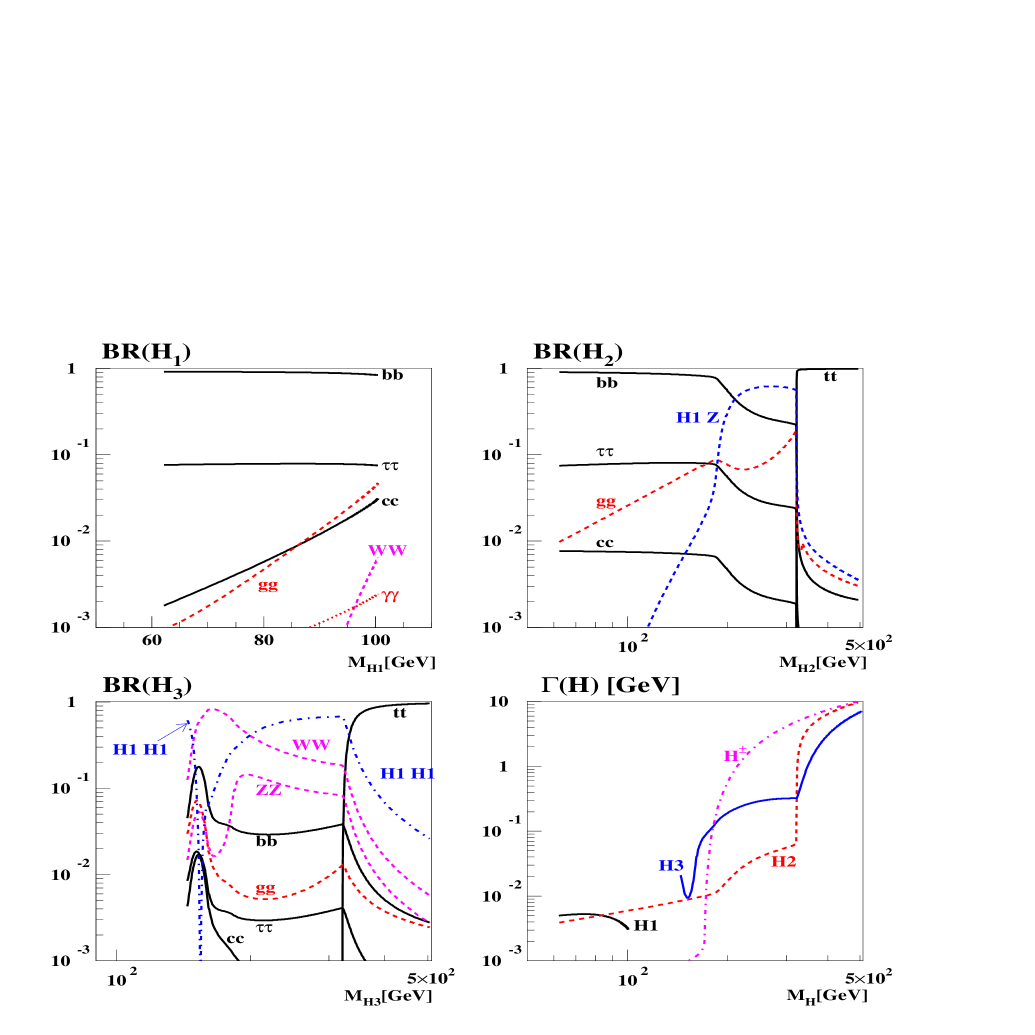
Figure 1: The branching ratios and total decay widths of the MSSM Higgs bosons, taking into account only the decays into SM particles. All the CP phases are set to zero and $\tan\beta=1.5$ is taken. For the comparison with HDECAY, the threshold corrections are not included and we assume the ‘maximal mixing’ scenario: $|A_{t,b,\tau}|=\sqrt{6}M_{\rm SUSY}$ with the common SUSY scale $M_{\rm SUSY}=M_{\tilde{Q}_{3}}=M_{\tilde{U}_{3}}=M_{\tilde{D}_{3}}=M_{\tilde{L}_{3}}=M_{\tilde{E}_{3}}=1$ TeV and $|\mu|=100$ GeV. The results are consistent with those from the code HDECAY.

In order to check whether the code ${\tt CPsuperH}$ generates numerical outputs consistent with those provided by the code HDECAY [29] in the CP–invariant case, we run the code ${\tt CPsuperH}$ in the ‘maximal mixing’ scenario: $|A_{t,b}|=\sqrt{6}M_{\rm SUSY}$ with the common SUSY scale $M_{\rm SUSY}=M_{\tilde{Q}_{3}}=M_{\tilde{U}_{3}}=M_{\tilde{D}_{3}}=M_{\tilde{L}_{3}}=M_{\tilde{E}_{3}}=1$ TeV and $|\mu|=100$ GeV, by setting all the CP phases to zeros, but not including the threshold corrections. Fig. 1 shows the branching ratios and total decay widths of the MSSM Higgs bosons as functions of the Higgs boson masses. Although most of the parameter space presented in Fig. 1 is already ruled out by Higgs searches at LEP, we use it to present an effective comparison of the results of the CPsuperH code with those of the HDECAY code in the small-$\tan\beta$ regime. We find that the CPsuperH results are indeed consistent with those obtained by the code HDECAY. There are very few visible discrepancies, for example in $B(H_{1}\rightarrow gg)$ for $M_{H_{1}}\raisebox{-3.69899pt}{~{}\shortstack{$<$ \\ [-0.07cm] $\sim$}}~{}80$ GeV, which may be due in part to the improved calculation of the Higgs-boson mass spectrum and the mixing matrix in CPsuperH.

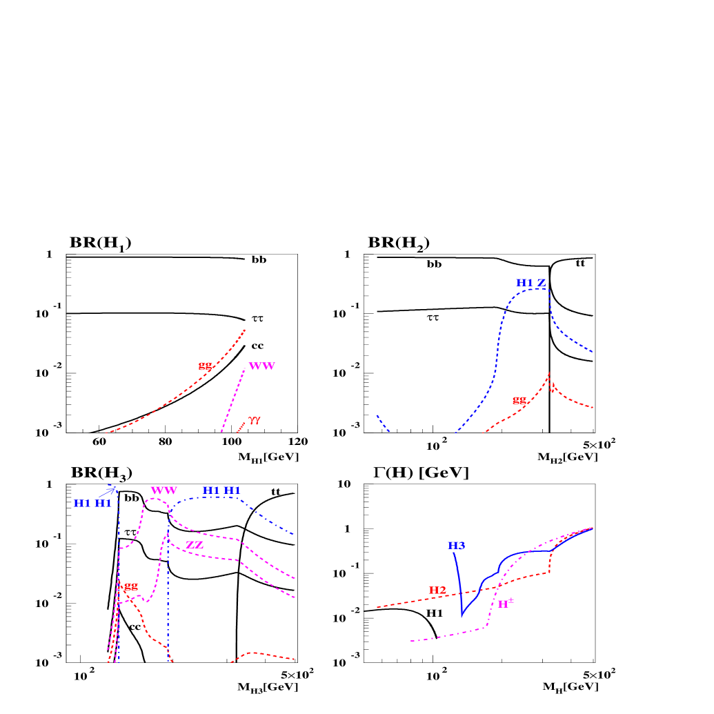
Figure 2: The branching ratios and total decay widths of the MSSM Higgs bosons, taking into account only the decays into SM particles. All the CP phases are set to zero and $\tan\beta=4$ is taken. We assume the CPX scenario: $|M_{3}|=1$ TeV, $|\mu|=4M_{\rm SUSY}$ and $|A_{t,b,\tau}|=2M_{\rm SUSY}$ with the common SUSY scale $M_{\rm SUSY}=M_{\tilde{Q}_{3}}=M_{\tilde{U}_{3}}=M_{\tilde{D}_{3}}=M_{\tilde{L}_{3}}=M_{\tilde{E}_{3}}=0.5$ TeV.

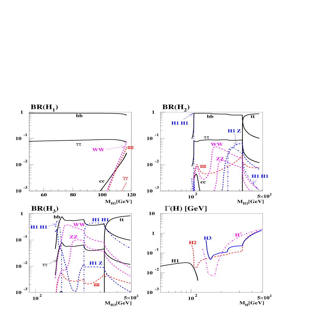
Figure 3: The same as in Fig. 2, but with non–trivial CP phases: $\Phi_{A_{t}}=\Phi_{A_{b}}=\Phi_{A_{\tau}}=\Phi_{3}=90^{\rm o}$.

We also show in Figs. 2 and 3 the branching ratios, GAMBRN(IM,2,IH), and total decay widths, GAMBRN(ISMN,1,IH) and GAMBRC(ISMC,1,IH), found in the CPX scenario, which are consistent with the results previously reported in [18]. Finally, in Fig. 4 we illustrate the strong phase dependence of the Higgs boson decay widths into charginos and neutralinos. The left frame is for the lightest neutral Higgs boson, which for the given choice of parameters can only decay into two lightest neutralinos, i.e. GAMBRN(ISMN+ISUSYN,3,1) = GAMBRN(ISMN+1,3,1). The right frame shows the branching ratios into superparticles of the heavier neutral Higgs bosons, GAMBRN(ISMN+ISUSYN,3,2) and GAMBRN(ISMN+ISUSYN,3,3), as well as the charged Higgs boson, GAMBRC(ISMC+ISUSYC,3), which only receive contributions from chargino/neutralino final states. The results of this figure are in close agreement with ref.[18].

4 Summary and Outlook

We have presented a detailed description of the Fortran code CPsuperH, a new computational package for studying Higgs phenomenology in the MSSM with explicit CP violation. Based on recent RG-improved diagrammatic calculations [23], the program CPsuperH computes the neutral and charged Higgs-boson masses as well as the $3\times 3$ neutral Higgs-boson mixing matrix $O$ in the presence of CP violation in the MSSM Higgs sector. Although the dominant one- and two-loop contributions to the Higgs-boson self-energies are incorporated, there are still finite but subdominant two-loop contributions that may cause shifts of 3–4 GeV [32, 36] in the lightest Higgs-boson mass. These subdominant contributions can be estimated [37] to be of comparable size with the dominant three-loop effects. Because of the current lack of a detailed three-loop calculation, the subdominant two–loop contributions are not included in the present version of the code CPsuperH.

In addition to the Higgs mass spectrum, the program CPsuperH computes all the couplings and the decay widths of the neutral Higgs bosons $H_{1,2,3}$ and the charged Higgs boson $H^{+}$, incorporating the most important quantum corrections [18, 24]. In particular, the leading-order QCD corrections are included for the Higgs decays into photons, gluons and most hadronic channels, so that (with the possible exception of squark final states) the theoretical uncertainties in these decay modes are kept small.

The Fortran code CPsuperH provides several options that can be selected in the input files for generating a variety of outputs for Higgs boson masses, Higgs decays and their respective branching fractions. Its structure offers the possibility of extending the list of input data to include flavour textures of off-diagonal trilinear and/or soft-squark masses, as these arise in some predictive schemes of soft SUSY breaking, e.g., in minimal supergravity models or in models with gauge and anomaly mediation. The code CPsuperH allows for straightforward extensions such as the additions of possible lepton- or quark-flavour-violating decays of the Higgs bosons. Another possible extension is the inclusion of loop–induced absorptive phases, which allows to generate CP–odd rate asymmetries in Higgs boson decays [38].

Radiative Higgs-sector CP violation in the MSSM has a wealth of implications for many different areas in particle-physics phenomenology. CP-violating phenomena mediated by Higgs-boson exchanges may manifest themselves in a number of low-energy observables such as the electron, neutron and muon electric dipole moments [39, 40, 41, 42]. They may also affect flavour-changing neutral-current processes and CP asymmetries involving $K$ and $B$ mesons [43, 33, 44]. Moreover, CP-violating Higgs effects may influence the annihilation rates of cosmic relics and hence the abundance of dark matter in the Universe [8]. Finally, an accurate determination of the Higgs spectrum in the presence of CP violation is crucial for testing the viability of electroweak baryogenesis in the MSSM.

To conclude, the Fortran code CPsuperH can be used as a powerful and efficient computational tool in quantitatively understanding these various phenomenological subjects, which are inter-related within the framework of the MSSM with explicit CP violation. Even in the CP-conserving case, CPsuperH is unique in computing the neutral and charged Higgs-boson couplings and masses with equally high level of precision, and should be therefore a useful tool for the study of MSSM Higgs phenomenology at present and future colliders.

Acknowledgements

We thank Eri Asakawa, Benedikt Gaissmaier, Kaoru Hagiwara, Stephen Mrenna and Jeonghyeon Song for fruitful collaborations. The work of SYC and MD was partially supported by the KOSEF–DFG Joint Research Project No. 20015-111-02-2. In addition, the work of SYC was supported in part by the Korea Research Foundation through the grant KRF–2002–070–C00022 and in part by KOSEF through CHEP at Kyungpook National University, and the work of MD was supported in part by the SFB375 of the Deutsche Forschungsgemeinschaft. Finally, the work of JSL and AP is supported in part by PPARC, under the grant no: PPA/G/O/2001/00461, and the work of CW is supported in part by the US DOE, Division of High Energy Physics, under the contract No. W-31-109-ENG-38.

Appendix A Threshold Corrections

The exchanges of gluinos and charginos give finite loop–induced threshold corrections to the Yukawa couplings $h_{u,d}$, with the structure

$$h_{d} = \frac{\sqrt{2}m_{d}}{v\cos\beta}\,\frac{1}{1+(\delta h_{d}/h_{d})+(\Delta h_{d}/h_{d})\tan\beta}\,,$$

$$h_{u} = \frac{\sqrt{2}m_{u}}{v\sin\beta}\,\frac{1}{1+(\delta h_{u}/h_{u})+(\Delta h_{u}/h_{u})\cot\beta}\,,$$ (A.1)

modifying the couplings of the neutral Higgs–boson mass eigenstate $H_{i}$ to the scalar and pseudoscalar fermion bilinears as follows:

$$g^{S}_{H_{i}\bar{d}d} = {\rm Re}\,\bigg{(}\,\frac{1}{1\,+\,\kappa_{d}\,\tan\beta}\,\bigg{)}\,\frac{O_{\phi_{1}i}}{\cos\beta}\ +\ {\rm Re}\,\bigg{(}\,\frac{\kappa_{d}}{1\,+\,\kappa_{d}\,\tan\beta}\,\bigg{)}\ \frac{O_{\phi 2i}}{\cos\beta}$$

$$+\>{\rm Im}\,\bigg{[}\,\frac{\kappa_{d}\,(\tan^{2}\beta\,+\,1)}{1\,+\,\kappa_{d}\,\tan\beta}\,\bigg{]}\ O_{ai}\,,$$

$$g^{P}_{H_{i}\bar{d}d} = -\,{\rm Re}\,\bigg{(}\,\frac{\tan\beta\,-\,\kappa_{d}}{1\,+\,\kappa_{d}\tan\beta}\,\bigg{)}\,O_{ai}\ +\ {\rm Im}\,\bigg{(}\,\frac{\kappa_{d}\,\tan\beta}{1\,+\,\kappa_{d}\,\tan\beta}\,\bigg{)}\ \frac{O_{\phi_{1}i}}{\cos\beta}$$ (A.2)

$$-\>{\rm Im}\,\bigg{(}\,\frac{\kappa_{d}}{1\,+\,\kappa_{d}\,\tan\beta}\,\bigg{)}\ \frac{O_{\phi 2i}}{\cos\beta}\ ,$$

$$g^{S}_{H_{i}\bar{u}u} = {\rm Re}\,\bigg{(}\,\frac{1}{1\,+\,\kappa_{u}\,\cot\beta}\,\bigg{)}\,\frac{O_{\phi 2i}}{\sin\beta}\ +\ {\rm Re}\,\bigg{(}\,\frac{\kappa_{u}}{1\,+\,\kappa_{u}\,\cot\beta}\,\bigg{)}\ \frac{O_{\phi_{1}i}}{\sin\beta}$$

$$+\>{\rm Im}\,\bigg{[}\,\frac{\kappa_{u}\,(\cot^{2}\beta\,+\,1)}{1\,+\,\kappa_{u}\,\cot\beta}\,\bigg{]}\ O_{ai}\,,$$

$$g^{P}_{H_{i}\bar{u}u} = -\,{\rm Re}\,\bigg{(}\,\frac{\cot\beta\,-\,\kappa_{u}}{1\,+\,\kappa_{u}\,\cot\beta}\,\bigg{)}\,O_{ai}\ +\ {\rm Im}\,\bigg{(}\,\frac{\kappa_{u}\,\cot\beta}{1\,+\,\kappa_{u}\,\cot\beta}\,\bigg{)}\ \frac{O_{\phi_{2}i}}{\sin\beta}$$ (A.3)

$$-\>{\rm Im}\,\bigg{(}\,\frac{\kappa_{u}}{1\,+\,\kappa_{u}\,\cot\beta}\,\bigg{)}\ \frac{O_{\phi_{1}i}}{\sin\beta}\ .$$

In the above equations, we have used the abbreviation

$$\kappa_{q}\ =\ \frac{(\Delta h_{q}/h_{q})}{1\>+\>(\delta h_{q}/h_{q})}\,,$$ (A.4)

for $q=u,d$. Detailed expressions for the threshold contributions $(\delta h_{q}/h_{q})$ and $(\Delta h_{q}/h_{q})$ can be found in [22].

For the couplings of the charged Higgs boson to quarks, we have

$$g^{L}_{H^{+}\bar{u}d} = \frac{\cot\beta\,(1\,+\,\rho_{u})\>-\>\bar{\kappa}_{u}}{1\>+\>\kappa_{u}\,\cot\beta}\ ,$$ (A.5)

$$g^{R}_{H^{+}\bar{u}d} = \frac{\tan\beta\,(1\,+\,\rho^{*}_{d})\>-\>\bar{\kappa}^{*}_{d}}{1\>+\>\kappa_{d}^{*}\,\tan\beta}\ .$$ (A.6)

The quantities $\kappa_{u,d}$ are given in (A.4), whilst the quantities $\bar{\kappa}_{u,d}$ and $\rho_{u,d}$ in (A.5) and (A.6) are defined as follows:

$$\bar{\kappa}_{q}\ =\ \frac{(\bar{\Delta}h_{q}/h_{q})}{1+(\delta h_{q}/h_{q})}\ ,\qquad\rho_{q}\ =\ \frac{(\bar{\delta}h_{q}/h_{q})\>-\>(\delta h_{q}/h_{q})}{1+(\delta h_{q}/h_{q})}\ .$$ (A.7)

The expressions for the additional threshold contributions $(\bar{\delta}h_{q}/h_{q})$ and $(\bar{\Delta}h_{q}/h_{q})$ can also be found in [22].

Appendix B Higgs–Boson Couplings to Third Generation Sfermions

Here we present the Higgs–sfermion–sfermion couplings in the weak-interaction basis. The couplings $\Gamma^{\alpha\tilde{f}^{*}\tilde{f}}$ are given in the $(\tilde{f}_{L},\tilde{f}_{R})$ basis by

$$\Gamma^{a\tilde{b}^{*}\tilde{b}} = \frac{1}{\sqrt{2}}\left(\begin{array}[]{cc}0&i\,h_{b}^{*}(s_{\beta}A_{b}^{*}+c_{\beta}\mu)\\ -i\,h_{b}(s_{\beta}A_{b}+c_{\beta}\mu^{*})&0\end{array}\right)\,,$$ (B.3)

$$\Gamma^{\phi_{1}\tilde{b}^{*}\tilde{b}} = \left(\begin{array}[]{cc}-|h_{b}|^{2}vc_{\beta}+\frac{1}{4}\left(g^{2}+\frac{1}{3}g^{\prime 2}\right)vc_{\beta}&-\frac{1}{\sqrt{2}}h_{b}^{*}A_{b}^{*}\\ -\frac{1}{\sqrt{2}}h_{b}A_{b}&-|h_{b}|^{2}vc_{\beta}+\frac{1}{6}g^{\prime 2}vc_{\beta}\end{array}\right)\,,$$ (B.6)

$$\Gamma^{\phi_{2}\tilde{b}^{*}\tilde{b}} = \left(\begin{array}[]{cc}-\frac{1}{4}\left(g^{2}+\frac{1}{3}g^{\prime 2}\right)vs_{\beta}&\frac{1}{\sqrt{2}}h_{b}^{*}\mu\\ \frac{1}{\sqrt{2}}h_{b}\mu^{*}&-\frac{1}{6}g^{\prime 2}vs_{\beta}\end{array}\right)\,,$$ (B.9)

$$\Gamma^{a\tilde{t}^{*}\tilde{t}} = \frac{1}{\sqrt{2}}\left(\begin{array}[]{cc}0&i\,h_{t}^{*}(c_{\beta}A_{t}^{*}+s_{\beta}\mu)\\ -i\,h_{t}(c_{\beta}A_{t}+s_{\beta}\mu^{*})&0\end{array}\right)\,,$$ (B.12)

$$\Gamma^{\phi_{1}\tilde{t}^{*}\tilde{t}} = \left(\begin{array}[]{cc}-\frac{1}{4}\left(g^{2}-\frac{1}{3}g^{\prime 2}\right)vc_{\beta}&\frac{1}{\sqrt{2}}h_{t}^{*}\mu\\ \frac{1}{\sqrt{2}}h_{t}\mu^{*}&-\frac{1}{3}g^{\prime 2}vc_{\beta}\end{array}\right)\,,$$ (B.15)

$$\Gamma^{\phi_{2}\tilde{t}^{*}\tilde{t}} = \left(\begin{array}[]{cc}-|h_{t}|^{2}vs_{\beta}+\frac{1}{4}\left(g^{2}-\frac{1}{3}g^{\prime 2}\right)vs_{\beta}&-\frac{1}{\sqrt{2}}h_{t}^{*}A_{t}^{*}\\ -\frac{1}{\sqrt{2}}h_{t}A_{t}&-|h_{t}|^{2}vs_{\beta}+\frac{1}{3}g^{\prime 2}vs_{\beta}\end{array}\right)\,,$$ (B.18)

$$\Gamma^{a\tilde{\tau}^{*}\tilde{\tau}} = \frac{1}{\sqrt{2}}\left(\begin{array}[]{cc}0&i\,h_{\tau}^{*}(s_{\beta}A_{\tau}^{*}+c_{\beta}\mu)\\ -i\,h_{\tau}(s_{\beta}A_{\tau}+c_{\beta}\mu^{*})&0\end{array}\right)\,,$$ (B.21)

$$\Gamma^{\phi_{1}\tilde{\tau}^{*}\tilde{\tau}} = \left(\begin{array}[]{cc}-|h_{\tau}|^{2}vc_{\beta}+\frac{1}{4}\left(g^{2}-g^{\prime 2}\right)vc_{\beta}&-\frac{1}{\sqrt{2}}h_{\tau}^{*}A_{\tau}^{*}\\ -\frac{1}{\sqrt{2}}h_{\tau}A_{\tau}&-|h_{\tau}|^{2}vc_{\beta}+\frac{1}{2}g^{\prime 2}vc_{\beta}\end{array}\right)\,,$$ (B.24)

$$\Gamma^{\phi_{2}\tilde{\tau}^{*}\tilde{\tau}} = \left(\begin{array}[]{cc}-\frac{1}{4}\left(g^{2}-g^{\prime 2}\right)vs_{\beta}&\frac{1}{\sqrt{2}}h_{\tau}^{*}\mu\\ \frac{1}{\sqrt{2}}h_{\tau}\mu^{*}&-\frac{1}{2}g^{\prime 2}vs_{\beta}\end{array}\right)\,,$$ (B.27)

$$\Gamma^{a\tilde{\nu}^{*}_{\tau}\tilde{\nu}_{\tau}} = 0\,,\qquad\Gamma^{\phi_{1}\tilde{\nu}^{*}_{\tau}\tilde{\nu}_{\tau}}=-\frac{1}{4}\left(g^{2}+g^{\prime 2}\right)vc_{\beta},\qquad\Gamma^{\phi_{2}\tilde{\nu}^{*}_{\tau}\tilde{\nu}_{\tau}}=\frac{1}{4}\left(g^{2}+g^{\prime 2}\right)vs_{\beta}\,.$$ (B.28)

The coupling $\Gamma^{H^{+}\tilde{u}^{*}\tilde{d}}$ is given in the LR basis by

$$\Gamma^{H^{+}\tilde{u}^{*}\tilde{d}}\ = \ \left(\begin{array}[]{cc}\frac{1}{\sqrt{2}}\,(|h_{u}|^{2}+|h_{d}|^{2}-g^{2})\,vs_{\beta}c_{\beta}&h_{d}^{*}\,(s_{\beta}A^{*}_{d}+c_{\beta}\mu)\\ h_{u}\,(c_{\beta}A_{u}+s_{\beta}\mu^{*})&\frac{1}{\sqrt{2}}\,h_{u}h^{*}_{d}\,v\end{array}\right)\,$$ (B.31)

$$\Gamma^{H^{+}\tilde{\nu}_{\tau}^{*}\tilde{\tau}_{L}}\ = \ \frac{1}{\sqrt{2}}\,(|h_{\tau}|^{2}-g^{2})\,vs_{\beta}\,c_{\beta}\,,\qquad\Gamma^{H^{+}\tilde{\nu}_{\tau}^{*}\tilde{\tau}_{R}}\ =\ h^{*}_{\tau}\left(s_{\beta}A^{*}_{\tau}+c_{\beta}\mu\right)$$ (B.32)

Appendix C Higgs–Boson Self–Couplings

In the following, we list all the effective trilinear and quartic Higgs–boson self–couplings of the Higgs weak eigenstates, which can be expressed in terms of the conventional quartic couplings $\lambda_{1,2,\dots,7}$ of the Higgs potential [13] obtained in an expansion of the effective Higgs potential up to operators of dimension 4. The trilinear couplings of the neutral Higgs bosons [18] are given by

$$g_{{}_{\phi_{1}\phi_{1}\phi_{1}}}\! = \!\!c_{\beta}\lambda_{1}\>+\>\frac{1}{2}\,s_{\beta}\,\Re{\rm e}\lambda_{6}\,,$$

$$g_{{}_{\phi_{1}\phi_{1}\phi_{2}}}\! = \!\!s_{\beta}\,\lambda_{34}\>+\>s_{\beta}\,\Re{\rm e}\lambda_{5}\>+\>\frac{3}{2}\,c_{\beta}\,\Re{\rm e}\lambda_{6}\,,$$

$$g_{{}_{\phi_{1}\phi_{2}\phi_{2}}}\! = \!\!c_{\beta}\,\lambda_{34}\>+\>c_{\beta}\,\Re{\rm e}\lambda_{5}\>+\>\frac{3}{2}\,s_{\beta}\,\Re{\rm e}\lambda_{7}\,,$$

$$g_{{}_{\phi_{2}\phi_{2}\phi_{2}}}\! = \!\!s_{\beta}\lambda_{2}\>+\>\frac{1}{2}\,c_{\beta}\,\Re{\rm e}\lambda_{7}\,,$$

$$g_{{}_{\phi_{1}\phi_{1}a}}\! = \!\!-s_{\beta}c_{\beta}\,\Im{\rm m}\lambda_{5}\>-\>\frac{1}{2}\,(1+2c^{2}_{\beta})\,\Im{\rm m}\lambda_{6}\,,$$

$$g_{{}_{\phi_{1}\phi_{2}a}}\! = \!\!-2\Im{\rm m}\lambda_{5}\>-\>s_{\beta}c_{\beta}\,\Im{\rm m}\,(\lambda_{6}+\lambda_{7})\,,$$

$$g_{{}_{\phi_{2}\phi_{2}a}}\! = \!\!-s_{\beta}c_{\beta}\,\Im{\rm m}\lambda_{5}\>-\>\frac{1}{2}\,(1+2s^{2}_{\beta})\,\Im{\rm m}\lambda_{7}\,,$$

$$g_{{}_{\phi_{1}aa}}\! = \!\!s^{2}_{\beta}c_{\beta}\lambda_{1}\>+\>c^{3}_{\beta}\,\lambda_{34}\>-\>c_{\beta}(1+s^{2}_{\beta})\,\Re{\rm e}\lambda_{5}\>+\>\frac{1}{2}\,s_{\beta}(s^{2}_{\beta}-2c^{2}_{\beta})\,\Re{\rm e}\lambda_{6}\>+\>\frac{1}{2}s_{\beta}c^{2}_{\beta}\,\Re{\rm e}\lambda_{7}\,,$$

$$g_{{}_{\phi_{2}aa}}\! = \!\!s_{\beta}c^{2}_{\beta}\lambda_{2}\>+\>s^{3}_{\beta}\,\lambda_{34}\>-\>s_{\beta}(1+c^{2}_{\beta})\,\Re{\rm e}\lambda_{5}\>+\>\frac{1}{2}s^{2}_{\beta}c_{\beta}\,\Re{\rm e}\lambda_{6}\>+\>\frac{1}{2}\,c_{\beta}(c^{2}_{\beta}-2s^{2}_{\beta})\,\Re{\rm e}\lambda_{7}\,,$$

$$g_{{}_{aaa}}\! = \!\!s_{\beta}c_{\beta}\,\Im{\rm m}\lambda_{5}\>-\>\frac{1}{2}\,s^{2}_{\beta}\,\Im{\rm m}\lambda_{6}\>-\>\frac{1}{2}\,c^{2}_{\beta}\,\Im{\rm m}\lambda_{7}\,,$$ (C.1)

with $\lambda_{34}=\frac{1}{2}\,(\lambda_{3}+\lambda_{4})$. The effective couplings $g_{{}_{\alpha H^{+}H^{-}}}$ [18] read:

$$g_{{}_{\phi_{1}H^{+}H^{-}}}\!\! = 2s^{2}_{\beta}c_{\beta}\lambda_{1}\>+\>c^{3}_{\beta}\lambda_{3}\>-\>s^{2}_{\beta}c_{\beta}\lambda_{4}\>-\>2s^{2}_{\beta}c_{\beta}\,\Re{\rm e}\lambda_{5}\>+\>s_{\beta}(s^{2}_{\beta}-2c^{2}_{\beta})\,\Re{\rm e}\lambda_{6}$$

$$+\>s_{\beta}c^{2}_{\beta}\Re{\rm e}\lambda_{7}\,,$$

$$g_{{}_{\phi_{2}H^{+}H^{-}}}\!\! = 2s_{\beta}c^{2}_{\beta}\lambda_{2}\>+\>s^{3}_{\beta}\lambda_{3}\>-\>s_{\beta}c^{2}_{\beta}\lambda_{4}\>-\>2s_{\beta}c^{2}_{\beta}\,\Re{\rm e}\lambda_{5}\>+\>s^{2}_{\beta}c_{\beta}\,\Re{\rm e}\lambda_{6}$$

$$+\>c_{\beta}(c^{2}_{\beta}-2s^{2}_{\beta})\,\Re{\rm e}\lambda_{7}\,,$$

$$g_{{}_{aH^{+}H^{-}}}\!\! = 2s_{\beta}c_{\beta}\,\Im{\rm m}\lambda_{5}\>-\>s^{2}_{\beta}\,\Im{\rm m}\lambda_{6}\>-\>c^{2}_{\beta}\,\Im{\rm m}\lambda_{7}\,.$$ (C.2)

The quartic couplings for the neutral Higgs bosons [22] are

$$g_{{}_{\phi_{1}\phi_{1}\phi_{1}\phi_{1}}}\! = \!\frac{1}{4}\,\lambda_{1}\,,\qquad g_{{}_{\phi_{1}\phi_{1}\phi_{1}\phi_{2}}}\ =\ \frac{1}{2}\,\Re{\rm e}\lambda_{6}\,,\qquad g_{{}_{\phi_{1}\phi_{1}\phi_{2}\phi_{2}}}\ =\ \frac{1}{2}\,\lambda_{34}\>+\>\frac{1}{2}\,\Re{\rm e}\lambda_{5}\,,$$

$$g_{{}_{\phi_{1}\phi_{2}\phi_{2}\phi_{2}}}\! = \!\frac{1}{2}\,\Re{\rm e}\lambda_{7}\,,\qquad g_{{}_{\phi_{2}\phi_{2}\phi_{2}\phi_{2}}}\ =\ \frac{1}{4}\,\lambda_{2}\,,$$

$$g_{{}_{\phi_{1}\phi_{1}\phi_{1}a}}\! = \!-\frac{1}{2}\,c_{\beta}\,\Im{\rm m}\lambda_{6}\,,\qquad g_{{}_{\phi_{1}\phi_{1}\phi_{2}a}}\ =\ -c_{\beta}\,\Im{\rm m}\lambda_{5}\>-\>\frac{1}{2}\,s_{\beta}\,\Im{\rm m}\lambda_{6}\,,$$

$$g_{{}_{\phi_{1}\phi_{2}\phi_{2}a}}\! = \!-s_{\beta}\,\Im{\rm m}\lambda_{5}\>-\>\frac{1}{2}\,c_{\beta}\,\Im{\rm m}\lambda_{7}\,,\qquad g_{{}_{\phi_{2}\phi_{2}\phi_{2}a}}\ =\ -\frac{1}{2}\,s_{\beta}\,\Im{\rm m}\lambda_{7}\,,$$

$$g_{{}_{\phi_{1}\phi_{1}aa}}\! = \!\frac{1}{2}\,s^{2}_{\beta}\,\lambda_{1}\>+\>\frac{1}{2}\,c^{2}_{\beta}\,\lambda_{34}\>-\>\frac{1}{2}\,c^{2}_{\beta}\,\Re{\rm e}\lambda_{5}\>-\>\frac{1}{2}\,s_{\beta}c_{\beta}\,\Re{\rm e}\lambda_{6}\,,$$

$$g_{{}_{\phi_{1}\phi_{2}aa}}\! = \!-2s_{\beta}c_{\beta}\,\Re{\rm e}\lambda_{5}\>+\>\frac{1}{2}\,s^{2}_{\beta}\,\Re{\rm e}\lambda_{6}\>+\>\frac{1}{2}\,c^{2}_{\beta}\,\Re{\rm e}\lambda_{7}\,,$$

$$g_{{}_{\phi_{2}\phi_{2}aa}}\! = \!\frac{1}{2}\,c^{2}_{\beta}\,\lambda_{2}\>+\>\frac{1}{2}\,s^{2}_{\beta}\,\lambda_{34}\>-\>\frac{1}{2}\,s^{2}_{\beta}\,\Re{\rm e}\lambda_{5}\>-\>\frac{1}{2}\,s_{\beta}c_{\beta}\,\Re{\rm e}\lambda_{7}\,,$$

$$g_{{}_{\phi_{1}aaa}}\! = \!s_{\beta}c^{2}_{\beta}\,\Im{\rm m}\lambda_{5}\>-\>\frac{1}{2}\,s^{2}_{\beta}c_{\beta}\,\Im{\rm m}\lambda_{6}\>-\>\frac{1}{2}\,c^{3}_{\beta}\,\Im{\rm m}\lambda_{7}\,,$$

$$g_{{}_{\phi_{2}aaa}}\! = \!s^{2}_{\beta}c_{\beta}\,\Im{\rm m}\lambda_{5}\>-\>\frac{1}{2}\,s^{3}_{\beta}\,\Im{\rm m}\lambda_{6}\>-\>\frac{1}{2}\,s_{\beta}c^{2}_{\beta}\,\Im{\rm m}\lambda_{7}\,,$$

$$g_{{}_{aaaa}}\! = \!\frac{1}{4}\,g_{{}_{H^{+}H^{-}H^{+}H^{-}}}\;,$$ (C.3)

with the quartic coupling of the charged Higgs bosons being given by

$$g_{{}_{H^{+}H^{-}H^{+}H^{-}}} = s^{4}_{\beta}\lambda_{1}\>+\>c^{4}_{\beta}\lambda_{2}\>+\>s^{2}_{\beta}c^{2}_{\beta}(\lambda_{3}+\lambda_{4})\>+\>2s^{2}_{\beta}c^{2}_{\beta}\Re{\rm e}\lambda_{5}\>-\>2s^{3}_{\beta}c_{\beta}\Re{\rm e}\lambda_{6}$$ (C.4)

$$-\>2s_{\beta}c^{3}_{\beta}\Re{\rm e}\lambda_{7}\,.$$

Finally, the remaining quartic couplings involving the charged Higgs boson pairs, $g_{\alpha\beta{\scriptscriptstyle H^{+}H^{-}}}$, are given by

$$g_{{}_{\phi_{1}\phi_{1}H^{+}H^{-}}}\! = \!s^{2}_{\beta}\,\lambda_{1}\>+\>\frac{1}{2}\,c^{2}_{\beta}\,\lambda_{3}\>-\>s_{\beta}c_{\beta}\,\Re{\rm e}\lambda_{6}\,,$$

$$g_{{}_{\phi_{1}\phi_{2}H^{+}H^{-}}}\! = \!-\,s_{\beta}c_{\beta}\,\lambda_{4}\>-\>2s_{\beta}c_{\beta}\,\Re{\rm e}\lambda_{5}\>+\>s^{2}_{\beta}\,\Re{\rm e}\lambda_{6}\>+\>c^{2}_{\beta}\,\Re{\rm e}\lambda_{7}\,,$$

$$g_{{}_{\phi_{2}\phi_{2}H^{+}H^{-}}}\! = \!c^{2}_{\beta}\,\lambda_{2}\>+\>\frac{1}{2}\,s^{2}_{\beta}\,\lambda_{3}\>-\>s_{\beta}c_{\beta}\,\Re{\rm e}\lambda_{7}\,,$$

$$g_{{}_{\phi_{1}aH^{+}H^{-}}}\! = \!2s_{\beta}c^{2}_{\beta}\,\Im{\rm m}\lambda_{5}\>-\>s^{2}_{\beta}c_{\beta}\,\Im{\rm m}\lambda_{6}\>-\>c^{3}_{\beta}\Im{\rm m}\lambda_{7}\,,$$

$$g_{{}_{\phi_{2}aH^{+}H^{-}}}\! = \!2s^{2}_{\beta}c_{\beta}\,\Im{\rm m}\lambda_{5}\>-\>s^{3}_{\beta}\,\Im{\rm m}\lambda_{6}\>-\>s_{\beta}c^{2}_{\beta}\Im{\rm m}\lambda_{7}\,,$$

$$g_{{}_{aaH^{+}H^{-}}}\! = \!g_{{}_{H^{+}H^{-}H^{+}H^{-}}}\;.$$ (C.5)

Appendix D Common Blocks

Here we list three common blocks for the SM and SUSY parameters, which are filled from two input arrays SMPARA_H and SSPARA_H.

• /HC_SMPARA/: This common block is for the SM parameters.

   COMMON /HC_SMPARA/ AEM_H,ASMZ_H,MZ_H,SW_H,ME_H,MMU_H,MTAU_H,MDMT_H
  .                                  ,MSMT_H,MBMT_H,MUMT_H,MCMT_H,MTPOLE_H,GAMW_H
  .                                  ,GAMZ_H,EEM_H,ASMT_H,CW_H,TW_H,MW_H,GW_H,GP_H
  .                                  ,V_H,GF_H,MTMT_H
  

  $$\begin{array}[]{lll}{\tt AEM\_H}=\alpha_{\rm em}(M_{Z})&{\tt ASMZ\_H}=\alpha_{s}(M_{Z})&{\tt MZ\_H}=M_{Z}\ [{\rm GeV}]\\ {\tt SW\_H}=\sin\theta_{W}&{\tt ME\_H}=m_{e}\ [{\rm GeV}]&{\tt MMU\_H}=m_{\mu}\ [{\rm GeV}]\\ {\tt MTAU\_H}=m_{\tau}\ [{\rm GeV}]&{\tt MDMT\_H}=m_{d}(m_{t}^{\rm pole})\ [{\rm GeV}]&{\tt MSMT\_H}=m_{s}(m_{t}^{\rm pole})\ [{\rm GeV}]\\ {\tt MBMT\_H}=m_{b}(m_{t}^{\rm pole})\ [{\rm GeV}]&{\tt MUMT\_H}=m_{u}(m_{t}^{\rm pole})\ [{\rm GeV}]&{\tt MCMT\_H}=m_{c}(m_{t}^{\rm pole})\ [{\rm GeV}]\\ {\tt MTPOLE\_H}=m_{t}^{\rm pole}\ [{\rm GeV}]&{\tt GAMW\_H}=\Gamma_{W}\ [{\rm GeV}]&{\tt GAMZ\_H}=\Gamma_{Z}\ [{\rm GeV}]\\ {\tt EEM\_H}=e=(4\pi\alpha_{\rm em}(M_{Z}))^{1/2}&{\tt ASMT\_H}=\alpha_{s}(m_{t}^{\rm pole})&{\tt CW\_H}=\cos\theta_{W}\\ {\tt TW\_H}=\tan\theta_{W}&{\tt MW\_H}=M_{W}=M_{Z}\cos\theta_{W}&{\tt GW\_H}=g=e/\sin\theta_{W}\\ {\tt GP\_H}=g^{\prime}=e/\cos\theta_{W}&{\tt V\_H}=2M_{W}/g&{\tt GF\_H}=G_{F}\\ {\tt MTMT\_H}=m_{t}(m_{t}^{\rm pole})\end{array}$$ (D.10)

  $$\alpha_{s}(m_{t}^{\rm pole}) = \frac{\alpha_{s}(M_{Z})}{1+\beta_{n_{f}}\frac{\alpha_{s}(M_{Z})}{4\pi}\ln(m_{t}^{\rm pole\,2}/M_{Z}^{2})}\ \ {\rm with}\ \ \beta_{n_{f}}=11-\frac{2}{3}n_{f}\,,$$

  $$G_{F} = \frac{\sqrt{2}g^{2}}{8M_{W}^{2}}\,,$$

  $$m_{t}(m_{t}^{\rm pole}) = \frac{m_{t}^{\rm pole}}{1+\frac{4\alpha_{s}(m_{t}^{\rm pole})}{3\pi}}\,.$$ (D.11)

• /HC_RSUSYPARA/: This is for the real SUSY parameters.

    COMMON /HC_RSUSYPARA/ TB_H,CB_H,SB_H,MQ3_H,MU3_H,MD3_H,ML3_H,ME3_H
  

  $$\begin{array}[]{llll}{\tt TB\_H}=\tan\beta&{\tt CB\_H}=\cos\beta&{\tt SB\_H}=\sin\beta&{\tt MQ3\_H}=M_{\tilde{Q}_{3}}\\ {\tt MU3\_H}=M_{\tilde{U}_{3}}&{\tt MD3\_H}=M_{\tilde{D}_{3}}&{\tt ML3\_H}=M_{\tilde{L}_{3}}&{\tt ME3\_H}=M_{\tilde{E}_{3}}\end{array}$$ (D.14)

• /HC_CSUSYPARA/: This is for the complex SUSY parameters.

    COMPLEX*16 MU_H,M1_H,M2_H,M3_H,AT_H,AB_H,ATAU_H
     COMMON /HC_CSUSYPARA/ MU_H,M1_H,M2_H,M3_H,AT_H,AB_H,ATAU_H

  $$\begin{array}[]{llll}{\tt MU\_H}=\mu\ [{\rm GeV}]&{\tt M1\_H}=M_{1}\ [{\rm GeV}]&{\tt M2\_H}=M_{2}\ [{\rm GeV}]&{\tt M3\_H}=M_{3}\ [{\rm GeV}]\\ {\tt AT\_H}=A_{t}\ [{\rm GeV}]&{\tt AB\_H}=A_{b}\ [{\rm GeV}]&{\tt ATAU\_H}=A_{\tau}\ [{\rm GeV}]&{}\end{array}$$ (D.17)

Appendix E Sample Outputs

Here we show the results of a test run of the code CPsuperH for the CPX scenario of MSSM Higgs-sector CP violation.

• ${\tt IFLAG\_H(1)}=1$: The list of the SM and SUSY input parameters
  ---------------------------------------------------------
  Standard Model Parameters in /HC_SMPARA/
  ---------------------------------------------------------
  AEM_H    = 0.7812E-02 : alpha_em(MZ)
  ASMZ_H   = 0.1172E+00 : alpha_s(MZ)
  MZ_H     = 0.9119E+02 : Z boson mass in GeV
  SW_H     = 0.4808E+00 : sinTheta_W
  ME_H     = 0.5000E-03 : electron mass in GeV
  MMU_H    = 0.1065E+00 : muon mass in GeV
  MTAU_H   = 0.1777E+01 : tau mass in GeV
  MDMT_H   = 0.6000E-02 : d-quark mass at M_t^pole in GeV
  MSMT_H   = 0.1150E+00 : s-quark mass at M_t^pole in GeV
  MBMT_H   = 0.3000E+01 : b-quark mass at M_t^pole in GeV
  MUMT_H   = 0.3000E-02 : u-quark mass at M_t^pole in GeV
  MCMT_H   = 0.6200E+00 : c-quark mass at M_t^pole in GeV
  MTPOLE_H = 0.1750E+03 : t-quark pole mass in GeV
  GAMW_H   = 0.2118E+01 : Gam_W in GeV
  GAMZ_H   = 0.2495E+01 : Gam_Z in GeV
  EEM_H    = 0.3133E+00 : e = (4*pi*alpha_em)^1/2
  ASMT_H   = 0.1072E+00 : alpha_s(M_t^pole)
  CW_H     = 0.8768E+00 : cosTheta_W
  TW_H     = 0.5483E+00 : tanTheta_W
  MW_H     = 0.7996E+02 : W boson mass MW = MZ*CW
  GW_H     = 0.6517E+00 : SU(2) gauge coupling gw=e/s_W
  GP_H     = 0.3573E+00 : U(1)_Y gauge coupling gp=e/c_W
  V_H      = 0.2454E+03 : V = 2 MW / gw
  GF_H     = 0.1174E-04 : GF=sqrt(2)*gw^2/8 MW^2 in GeV^2
  MTMT_H   = 0.1674E+03 : t-quark mass at M_t^pole in GeV
  ---------------------------------------------------------
  Real SUSY Parameters in /HC_RSUSYPARA/
  ---------------------------------------------------------
  TB_H     = 0.5000E+01 : tan(beta)
  CB_H     = 0.1961E+00 : cos(beta)
  SB_H     = 0.9806E+00 : sin(beta)
  MQ3_H    = 0.5000E+03 : M_tildeQ_3 in GeV
  MU3_H    = 0.5000E+03 : M_tildeU_3 in GeV
  MD3_H    = 0.5000E+03 : M_tildeD_3 in GeV
  ML3_H    = 0.5000E+03 : M_tildeL_3 in GeV
  ME3_H    = 0.5000E+03 : M_tildeE_3 in GeV
  ---------------------------------------------------------
  Complex SUSY Parameters in /HC_CSUSYPARA/
  ---------------------------------------------------------
  |MU_H|     = 0.2000E+04:Mag. of MU parameter in GeV
  |M1_H|     = 0.5000E+02:Mag. of M1 parameter in GeV
  |M2_H|     = 0.1000E+03:Mag. of M2 parameter in GeV
  |M3_H|     = 0.1000E+04:Mag. of M3 parameter in GeV
  |AT_H|     = 0.1000E+04:Mag. of AT parameter in GeV
  |AB_H|     = 0.1000E+04:Mag. of AB parameter in GeV
  |ATAU_H|   = 0.1000E+04:Mag. of ATAU parameter in GeV
  ARG(MU_H)  = 0.0000E+00:Arg. of MU parameter in Degree
  ARG(M1_H)  = 0.0000E+00:Arg. of M1 parameter in Degree
  ARG(M2_H)  = 0.0000E+00:Arg. of M2 parameter in Degree
  ARG(M3_H)  = 0.9000E+02:Arg. of M3 parameter in Degree
  ARG(AT_H)  = 0.9000E+02:Arg. of AT parameter in Degree
  ARG(AB_H)  = 0.9000E+02:Arg. of AB parameter in Degree
  ARG(ATAU_H)= 0.9000E+02:Arg. of ATAU parameter in Degree
  ---------------------------------------------------------
  Charged Higgs boson pole mass : 0.3000E+03 GeV
  ---------------------------------------------------------
  

• ${\tt IFLAG\_H(2)}=1$: The masses and mixing matrix of the neutral Higgs bosons
  ---------------------------------------------------------
  Masses and Mixing Matrix of Higgs bosons :
                                 HMASS_H(I) and OMIX_H(A,I)
  ---------------------------------------------------------
  H1  Pole Mass           = 0.1188E+03 GeV
  H2  Pole Mass           = 0.2703E+03 GeV
  H3  Pole Mass           = 0.2981E+03 GeV
  Charged Higgs Pole Mass = 0.3000E+03 GeV [SSPARA_H(2)]
                           [H1]       [H2]       [H3]
            [phi_1] / 0.2451E+00 -.3373E+00 -.9089E+00 $\backslash$ 
  O(IA,IH)=[phi_2] | 0.9694E+00 0.7532E-01 0.2335E+00 |
              [ a ] $\backslash$ -.1030E-01 -.9384E+00 0.3454E+00 /
  ---------------------------------------------------------
  

• ${\tt IFLAG\_H(4)}=1$: The masses and mixing matrices of the charginos and neutralinos
  ---------------------------------------------------------
  Chargino Masses and Mixing Matrices :
                          MC_H(I), UL_H(I,A), and UR_H(I,A)
  ---------------------------------------------------------
  MC1 = 0.9861E+02 GeV      MC2 = 0.2003E+04 GeV
  
  UL_H =
  /(0.9984E+00 0.0000E+00) (-.5603E-01 0.0000E+00) $\backslash$
  $\backslash$(0.5603E-01 0.0000E+00) (0.9984E+00 0.0000E+00) /
  
  UR_H =
  /(0.9999E+00 0.0000E+00) (-.1385E-01 0.5460E-09) $\backslash$
  $\backslash$(0.1385E-01 0.0000E+00) (0.9999E+00 0.0000E+00) /
  ---------------------------------------------------------
  Neutralino Masses MN_H(I) and Mixing Matrix N_H(I,A)
  ---------------------------------------------------------
  MN1 = 0.4960E+02 GeV      MN2 = 0.9862E+02 GeV
  MN3 = 0.2001E+04 GeV      MN4 = 0.2003E+04 GeV
  
  N_H(1,1) = (0.9996E+00 0.0000E+00)
  N_H(1,2) = (-.1462E-01 0.0000E+00)
  N_H(1,3) = (0.2218E-01 0.0000E+00)
  N_H(1,4) = (-.4962E-02 0.0000E+00)
  
  N_H(2,1) = (-.1553E-01 0.0000E+00)
  N_H(2,2) = (-.9991E+00 0.0000E+00)
  N_H(2,3) = (0.3931E-01 0.0000E+00)
  N_H(2,4) = (-.9704E-02 0.0000E+00)
  
  N_H(3,1) = (0.0000E+00 -.1186E-01)
  N_H(3,2) = (0.0000E+00 0.2112E-01)
  N_H(3,3) = (0.0000E+00 0.7066E+00)
  N_H(3,4) = (0.0000E+00 0.7072E+00)
  
  N_H(4,1) = (0.1867E-01 0.0000E+00)
  N_H(4,2) = (-.3494E-01 0.0000E+00)
  N_H(4,3) = (-.7062E+00 0.0000E+00)
  N_H(4,4) = (0.7069E+00 0.0000E+00)
  ---------------------------------------------------------
  

• ${\tt IFLAG\_H(5)}=1$: The couplings of the lightest Higgs boson
  ---------------------------------------------------------
  The Lightest Higgs H_1 Couplings : NHC_H(NC,1)
  ---------------------------------------------------------
  H1 e e               [NC= 1]: GF=(0.2038E-05,0.0000E+00)
                        [NC= 2]: GS=(0.1250E+01,0.0000E+00)
                        [NC= 3]: GP=(0.5148E-01,0.0000E+00)
  H1 mu mu             [NC= 4]: GF=(0.4340E-03,0.0000E+00)
                        [NC= 5]: GS=(0.1250E+01,0.0000E+00)
                        [NC= 6]: GP=(0.5148E-01,0.0000E+00)
  H1 tau tau           [NC= 7]: GF=(0.7242E-02,0.0000E+00)
                        [NC= 8]: GS=(0.1250E+01,0.0000E+00)
                        [NC= 9]: GP=(0.5148E-01,0.0000E+00)
  H1 d d               [NC=10]: GF=(0.2445E-04,0.0000E+00)
                        [NC=11]: GS=(0.1250E+01,0.0000E+00)
                        [NC=12]: GP=(0.5148E-01,0.0000E+00)
  H1 s s               [NC=13]: GF=(0.4687E-03,0.0000E+00)
                        [NC=14]: GS=(0.1250E+01,0.0000E+00)
                        [NC=15]: GP=(0.5148E-01,0.0000E+00)
  H1 b b               [NC=16]: GF=(0.1223E-01,0.0000E+00)
                        [NC=17]: GS=(0.1246E+01,0.0000E+00)
                        [NC=18]: GP=(-.1741E-01,0.0000E+00)
  H1 u u               [NC=19]: GF=(0.1223E-04,0.0000E+00)
                        [NC=20]: GS=(0.9886E+00,0.0000E+00)
                        [NC=21]: GP=(0.2059E-02,0.0000E+00)
  H1 c c               [NC=22]: GF=(0.2527E-02,0.0000E+00)
                        [NC=23]: GS=(0.9886E+00,0.0000E+00)
                        [NC=24]: GP=(0.2059E-02,0.0000E+00)
  H1 t t               [NC=25]: GF=(0.6821E+00,0.0000E+00)
                        [NC=26]: GS=(0.9892E+00,0.0000E+00)
                        [NC=27]: GP=(0.4501E-02,0.0000E+00)
  H1 N1 N1             [NC=28]: GF=(0.3258E+00,0.0000E+00)
                        [NC=29]: GS=(-.5767E-02,0.0000E+00)
                        [NC=30]: GP=(0.1317E-03,0.0000E+00)
  H1 N2 N2             [NC=31]: GF=(0.3258E+00,0.0000E+00)
                        [NC=32]: GS=(-.1886E-01,0.0000E+00)
                        [NC=33]: GP=(0.4125E-03,0.0000E+00)
  H1 N3 N3             [NC=34]: GF=(0.3258E+00,0.0000E+00)
                        [NC=35]: GS=(0.1415E-01,0.0000E+00)
                        [NC=36]: GP=(0.1576E-03,0.0000E+00)
  H1 N4 N4             [NC=37]: GF=(0.3258E+00,0.0000E+00)
                        [NC=38]: GS=(0.3878E-01,0.0000E+00)
                        [NC=39]: GP=(-.3866E-03,0.0000E+00)
  H1 N1 N2             [NC=40]: GF=(0.3258E+00,0.0000E+00)
                        [NC=41]: GS=(-.1043E-01,0.0000E+00)
                        [NC=42]: GP=(0.2331E-03,0.0000E+00)
  H1 N1 N3             [NC=43]: GF=(0.3258E+00,0.0000E+00)
                        [NC=44]: GS=(-.1602E-02,0.0000E+00)
                        [NC=45]: GP=(0.1443E+00,0.0000E+00)
  H1 N1 N4             [NC=46]: GF=(0.3258E+00,0.0000E+00)
                        [NC=47]: GS=(0.2413E+00,0.0000E+00)
                        [NC=48]: GP=(-.2402E-02,0.0000E+00)
  H1 N2 N3             [NC=49]: GF=(0.3258E+00,0.0000E+00)
                        [NC=50]: GS=(-.2820E-02,0.0000E+00)
                        [NC=51]: GP=(0.2540E+00,0.0000E+00)
  H1 N2 N4             [NC=52]: GF=(0.3258E+00,0.0000E+00)
                        [NC=53]: GS=(0.4247E+00,0.0000E+00)
                        [NC=54]: GP=(-.4228E-02,0.0000E+00)
  H1 N3 N4             [NC=55]: GF=(0.3258E+00,0.0000E+00)
                        [NC=56]: GS=(-.2470E-03,0.0000E+00)
                        [NC=57]: GP=(-.2789E-03,0.0000E+00)
  H1 C1+ C1-           [NC=58]: GF=(0.4608E+00,0.0000E+00)
                        [NC=59]: GS=(-.2714E-01,0.0000E+00)
                        [NC=60]: GP=(0.5936E-03,-.2135E-18)
  H1 C1+ C2-           [NC=61]: GF=(0.4608E+00,0.0000E+00)
                        [NC=62]: GS=(0.6058E+00,0.4035E-02)
                        [NC=63]: GP=(-.6042E-02,-.3618E+00)
  H1 C2+ C1-           [NC=64]: GF=(0.4608E+00,0.0000E+00)
                        [NC=65]: GS=(0.6058E+00,-.4035E-02)
                        [NC=66]: GP=(-.6042E-02,0.3618E+00)
  H1 C2+ C2-           [NC=67]: GF=(0.4608E+00,0.0000E+00)
                        [NC=68]: GS=(0.5771E-01,0.0000E+00)
                        [NC=69]: GP=(-.2527E-03,0.7454E-19)
  H1 V V               [NC=70]: G =(0.9987E+00,0.0000E+00)
  H1 ST1* ST1          [NC=71]: G =(0.2184E+01,-.3755E-16)
  H1 ST1* ST2          [NC=72]: G =(0.2447E+00,-.1144E+00)
  H1 ST2* ST1          [NC=73]: G =(0.2447E+00,0.1144E+00)
  H1 ST2* ST2          [NC=74]: G =(-.3987E+01,-.4869E-17)
  H1 SB1* SB1          [NC=75]: G =(0.4330E+00,0.1506E-18)
  H1 SB1* SB2          [NC=76]: G =(0.2070E-01,0.8020E-02)
  H1 SB2* SB1          [NC=77]: G =(0.2070E-01,-.8020E-02)
  H1 SB2* SB2          [NC=78]: G =(-.5584E+00,0.1683E-18)
  H1 STA1* STA1        [NC=79]: G =(0.2300E+00,-.1144E-17)
  H1 STA1* STA2        [NC=80]: G =(0.1602E-02,0.6836E-02)
  H1 STA2* STA1        [NC=81]: G =(0.1602E-02,-.6836E-02)
  H1 STA2* STA2        [NC=82]: G =(-.3549E+00,-.1785E-17)
  H1 SNU3* SNU3        [NC=83]: G =(0.1246E+00,0.0000E+00)
  H1 glue glue         [NC=84]: S =(0.5827E+00,0.3665E-01)
                        [NC=85]: P =(0.5195E-02,-.5135E-03)
  H1 CH+ CH-           [NC=86]: G =(-.4047E-01,0.0000E+00)
  H1 CH+ W-            [NC=87]: G =(-.5024E-01,0.1030E-01)
  H1 photon photon     [NC=88]: S =(-.6557E+01,0.2443E-01)
                        [NC=89]: P =(0.1385E-01,-.3423E-03)
  H1 glue glue    (M=0)[NC=90]: S =(0.1427E+01,0.1915E-17)
                        [NC=91]: P =(-.1291E-01,0.0000E+00)
  H1 photon photon(M=0)[NC=92]: S =(-.4878E+01,0.5235E-17)
                        [NC=93]: P =(0.1728E-02,-.4811E-18)
  ---------------------------------------------------------
  

• ${\tt IFLAG\_H(6)}=1$: The decay width and branching fractions of the lightest Higgs boson
  ---------------------------------------------------------
  Neutral Higgs Boson Decays with ISMN =  50 : ISUSYN =  50
  ---------------------------------------------------------
  DECAY MODE    [ IM]   WIDTH[GeV]  BR[SM]      BR[TOTAL]
  ---------------------------------------------------------
  H1 -> e    e  [  1]:  0.3070E-10  0.5766E-08  0.5760E-08
  H1 -> mu   mu [  2]:  0.1393E-05  0.2616E-03  0.2613E-03
  H1 -> tau  tau[  3]:  0.3873E-03  0.7274E-01  0.7266E-01
  H1 -> d    d  [  4]:  0.1686E-07  0.3166E-05  0.3163E-05
  H1 -> s    s  [  5]:  0.6193E-05  0.1163E-02  0.1162E-02
  H1 -> b    b  [  6]:  0.4163E-02  0.7820E+00  0.7812E+00
  H1 -> u    u  [  7]:  0.2632E-08  0.4944E-06  0.4939E-06
  H1 -> c    c  [  8]:  0.1124E-03  0.2111E-01  0.2109E-01
  H1 -> t    t  [  9]:  0.0000E+00  0.0000E+00  0.0000E+00
  H1 -> W    W  [ 10]:  0.4106E-03  0.7711E-01  0.7703E-01
  H1 -> Z    Z  [ 11]:  0.3303E-04  0.6203E-02  0.6197E-02
  H1 -> H1   Z  [ 12]:  0.0000E+00  0.0000E+00  0.0000E+00
  H1 -> H2   Z  [ 13]:  0.0000E+00  0.0000E+00  0.0000E+00
  H1 -> H1   H1 [ 14]:  0.0000E+00  0.0000E+00  0.0000E+00
  H1 -> H1   H2 [ 15]:  0.0000E+00  0.0000E+00  0.0000E+00
  H1 -> H2   H2 [ 16]:  0.0000E+00  0.0000E+00  0.0000E+00
  H1 -> ph   ph [ 17]:  0.9427E-05  0.1771E-02  0.1769E-02
  H1 -> gl   gl [ 18]:  0.2004E-03  0.3763E-01  0.3760E-01
  H1 TOTAL(SM)  [ 50]:  0.5324E-02  0.1000E+01  0.9990E+00
  H1 -> N1   N1 [ 51]:  0.5557E-05  0.1044E-02  0.1043E-02
  H1 -> N1   N2 [ 52]:  0.0000E+00  0.0000E+00  0.0000E+00
  H1 -> N1   N3 [ 53]:  0.0000E+00  0.0000E+00  0.0000E+00
  H1 -> N1   N4 [ 54]:  0.0000E+00  0.0000E+00  0.0000E+00
  H1 -> N2   N2 [ 55]:  0.0000E+00  0.0000E+00  0.0000E+00
  H1 -> N2   N3 [ 56]:  0.0000E+00  0.0000E+00  0.0000E+00
  H1 -> N2   N4 [ 57]:  0.0000E+00  0.0000E+00  0.0000E+00
  H1 -> N3   N3 [ 58]:  0.0000E+00  0.0000E+00  0.0000E+00
  H1 -> N3   N4 [ 59]:  0.0000E+00  0.0000E+00  0.0000E+00
  H1 -> N4   N4 [ 60]:  0.0000E+00  0.0000E+00  0.0000E+00
  H1 -> C1+  C1-[ 61]:  0.0000E+00  0.0000E+00  0.0000E+00
  H1 -> C1+  C2-[ 62]:  0.0000E+00  0.0000E+00  0.0000E+00
  H1 -> C2+  C1-[ 63]:  0.0000E+00  0.0000E+00  0.0000E+00
  H1 -> C2+  C2-[ 64]:  0.0000E+00  0.0000E+00  0.0000E+00
  H1 -> ST1* ST1[ 65]:  0.0000E+00  0.0000E+00  0.0000E+00
  H1 -> ST1* ST2[ 66]:  0.0000E+00  0.0000E+00  0.0000E+00
  H1 -> ST2* ST1[ 67]:  0.0000E+00  0.0000E+00  0.0000E+00
  H1 -> ST2* ST2[ 68]:  0.0000E+00  0.0000E+00  0.0000E+00
  H1 -> SB1* SB1[ 69]:  0.0000E+00  0.0000E+00  0.0000E+00
  H1 -> SB1* SB2[ 70]:  0.0000E+00  0.0000E+00  0.0000E+00
  H1 -> SB2* SB1[ 71]:  0.0000E+00  0.0000E+00  0.0000E+00
  H1 -> SB2* SB2[ 72]:  0.0000E+00  0.0000E+00  0.0000E+00
  H1 ->STA1*STA1[ 73]:  0.0000E+00  0.0000E+00  0.0000E+00
  H1 ->STA1*STA2[ 74]:  0.0000E+00  0.0000E+00  0.0000E+00
  H1 ->STA2*STA1[ 75]:  0.0000E+00  0.0000E+00  0.0000E+00
  H1 ->STA2*STA2[ 76]:  0.0000E+00  0.0000E+00  0.0000E+00
  H1 ->SNU3*SNU3[ 77]:  0.0000E+00  0.0000E+00  0.0000E+00
  H1 TOTAL(SUSY)[100]:  0.5557E-05  0.1044E-02  0.1043E-02
  H1 TOTAL      [101]:  0.5330E-02  0.1001E+01  0.1000E+01
  
  $*$ Note : WIDTH=GAMBRN(IM,1,1), BR[SM]   =GAMBRN(IM,2,1)
                         and      BR[TOTAL]=GAMBRN(IM,3,1)
  ---------------------------------------------------------
  

Figure 4: The dependence of the branching ratios of Higgs bosons into superparticles on the phase $\phi_{\mu}$, for $\tan\beta=5,\,M_{H^{+}}^{\rm pole}=0.3$ TeV, $M_{\tilde{Q}_{3}}=M_{\tilde{U}_{3}}=M_{\tilde{D}_{3}}=M_{\tilde{L}_{3}}=M_{\tilde{E}_{3}}=0.5$ TeV, $|\mu|=250$ GeV, $|M_{1}|=50$ GeV, $|M_{2}|=150$ GeV, $|M_{3}|=0.5$ TeV, $|A_{t}|=|A_{b}|=|A_{\tau}|=1.2$ TeV, $\Phi_{2}=\Phi_{3}=0$, and $\Phi_{A_{t}}=\Phi_{A_{b}}=\Phi_{A_{\tau}}=-\Phi_{\mu}$. The left frame shows results for $H_{1}$ for several choices of $\Phi_{1}$; in this case the only contributing final state is $\tilde{\chi}_{1}^{0}\tilde{\chi}_{1}^{0}$. The right frame shows results for the heavier Higgs bosons, where the solid (dotted) lines are for $\Phi_{1}=0\ (180^{\circ})$; in this case heavier neutralinos and charginos contribute, but no sfermions.

References

- [1] P.W. Higgs, Phys. Rev. Lett. 12 (1964) 132; P.W. Higgs, Phys. Rev. 145 (1966) 1156; F. Englert and R. Brout, Phys. Rev. Lett. 13 (1964) 321; G.S. Guralnik, C.R. Hagen, and T.W. Kibble, Phys. Rev. Lett. 13 (1964) 585.
- [2] L. Maiani, Proceedings of the 1979 Gif-sur-Yvette Summer School On Particle Physics, 1; G. ’t Hooft, in Recent Developments in Gauge Theories, Proceedings of the Nato Advanced Study Institute, Cargese, 1979, eds. G. ’t Hooft et al., (Plenum Press, NY, 1980); E. Witten, Phys. Lett. B 105 (1981) 267.
- [3] For reviews, see, H.P. Nilles, Phys. Rep. 110 (1984) 1; H. Haber and G. Kane, Phys. Rep. 117 (1985) 75; J.F. Gunion, H.E. Haber, G.L. Kane and S. Dawson, The Higgs Hunter’s Guide, (Addison-Wesley, Reading, MA, 1990).
- [4] S. Dimopoulos and H. Georgi, Nucl. Phys. B193 (1981) 150; S. Dimopoulos, S. Raby and F. Wilczek, Phys. Rev. D24 (1981) 1681; L. E. Ibáñez and G. G. Ross, Phys. Lett. B 105 (1981) 439; J. Ellis, S. Kelley and D. V. Nanopoulos, Phys. Lett. B 260 (1991) 131; U. Amaldi, W. de Boer and H. Fürstenau, Phys. Lett. B 260 (1991) 447; P. Langacker and M.-X. Luo, Phys. Rev. D 44 (1991) 817; C. Giunti, C. W. Kim and U. W. Lee, Mod. Phys. Lett. A 6 (1991) 1745; M. Carena, S. Pokorski and C.E.M. Wagner, Nucl. Phys. B406 (1993) 59.
- [5] V.A. Kuzmin, V.A. Rubakov and M.E. Shaposhnikov, Phys. Lett. B155 (1985) 36.
- [6] For recent studies, see, M. Carena, M. Quirós and C.E.M. Wagner, Nucl. Phys. B524 (1998) 3; M. Laine and K. Rummukainen, Phys. Rev. Lett. 80 (1998) 5259 and Nucl. Phys. B535 (1998) 423; K. Funakubo, Prog. Theor. Phys. 101 (1999) 415 and 102 (1999) 389; J. Grant and M. Hindmarsh, Phys. Rev. D59 (1999) 116014; M. Losada, Nucl. Phys. B569 (2000) 125; S. Davidson, M. Losada and A. Riotto, Phys. Rev. Lett. 84 (2000) 4284; A.B. Lahanas, V.C. Spanos and V. Zarikas, Phys. Lett. B472 (2000) 119; J. M. Cline, M. Joyce and K. Kainulainen, JHEP 0007 (2000) 018; M. Carena, J.M. Moreno, M. Quiros, M. Seco and C.E.M. Wagner, Nucl. Phys. B599 (2001) 158; M. Laine and K. Rummukainen, Nucl. Phys. B597 (2001) 23; S.J. Huber, P. John and M.G. Schmidt, Eur. Phys. J. C 20 (2001) 695; K. Kainulainen, T. Prokopec, M. G. Schmidt and S. Weinstock, JHEP 0106 (2001) 031.
- [7] H. Goldberg, Phys. Rev. Lett. 50 (1983) 1419; J. Ellis, J.S. Hagelin, D.V. Nanopoulos, K.A. Olive and M. Srednicki, Nucl. Phys. B238 (1984) 453; M. Drees and M.M. Nojiri, Phys. Rev. D 47 (1993) 376; M.E. Gómez, G. Lazarides and C. Pallis, Phys. Lett. B487 (2000) 313; J. R. Ellis, T. Falk, G. Ganis, K. A. Olive and M. Srednicki, Phys. Lett. B510 (2001) 236.
- [8] P. Gondolo and K. Freese, hep-ph/990839; T. Falk, A. Ferstl and K.A. Olive, Astropart. Phys. 13 (2000) 301; S.Y. Choi, S.-C. Park, J.H. Jang and H.S. Song, Phys. Rev. D64 (2001) 015006.
- [9] M.S. Berger, Phys. Rev. D41 (1990) 225; J. Ellis, G. Ridolfi and F. Zwirner, Phys. Lett. B257 (1991) 83; Y. Okada, M. Yamaguchi and T. Yanagida, Prog. Theor. Phys. 85 (1991) 1; Phys. Lett. B262 (1991) 54; H.E. Haber and R. Hempfling, Phys. Rev. Lett. 66 (1991) 1815.
- [10] ALEPH, DELPHI, L3 and OPAL Collaborations, LEP Electroweak Working Group, SLD Heavy Flavor Group and SLD Electroweak Group, LEPEWWG/2003-01, available from http://lepewwg.web.cern.ch/LEPEWWG/stanmod/.
- [11] See, for example, G.-C. Cho and K. Hagiwara, Nucl. Phys. B574 (2000) 623.
- [12] A. Pilaftsis, Phys. Rev. D58 (1998) 096010 and Phys. Lett. B435 (1998) 88.
- [13] A. Pilaftsis and C.E.M. Wagner, Nucl. Phys. B553 (1999) 3.
- [14] D.A. Demir, Phys. Rev. D60 (1999) 055006.
- [15] S.Y. Choi, M. Drees and J.S. Lee, Phys. Lett. B481 (2000) 57.
- [16] M. Carena, J. Ellis, A. Pilaftsis and C.E.M. Wagner, Nucl. Phys. B586 (2000) 92.
- [17] G.L. Kane and L.-T. Wang, Phys. Lett. B488 (2000) 383.
- [18] S.Y. Choi and J.S. Lee, Phys. Rev. D61 (2000) 015003; S.Y. Choi, K. Hagiwara and J.S. Lee, Phys. Rev. D64 (2001) 032004; S. Y. Choi, M. Drees, J. S. Lee and J. Song, Eur. Phys. J. C 25 (2002) 307.
- [19] T. Ibrahim and P. Nath, Phys. Rev. D63 (2001) 035009; Phys. Rev. D66 (2002) 015005; T. Ibrahim, Phys. Rev. D64 (2001) 035009; S. W. Ham, S. K. Oh, E. J. Yoo, C. M. Kim and D. Son, hep-ph/0205244.
- [20] M. Carena, J. Ellis, A. Pilaftsis and C.E.M. Wagner, Phys. Lett. B495 (2000) 155.
- [21] S. Heinemeyer, Eur. Phys. J. C 22 (2001) 521.
- [22] M. Carena, J. Ellis, S. Mrenna, A. Pilaftsis and C.E.M. Wagner, hep-ph/0211467.
- [23] M. Carena, J. Ellis, A. Pilaftsis and C.E.M. Wagner, Nucl. Phys. B625 (2002) 345.
- [24] A. Dedes and S. Moretti, Phys. Rev. Lett. 84 (2000) 22; Nucl. Phys. B576 (2000) 29; S.Y. Choi and J.S. Lee, Phys. Rev. D61 (2000) 115002; S.Y. Choi, K. Hagiwara and J.S. Lee, Phys. Lett. B529 (2002) 212; A. Arhrib, D. K. Ghosh and O.C. Kong, Phys. Lett. B537 (2002) 217.
- [25] B.E. Cox, J.R. Forshaw, J.S. Lee, J.W. Monk and A. Pilaftsis, hep-ph/0303206; A.G. Akeroyd, hep-ph/0306045.
- [26] B. Grzadkowski, J. F. Gunion and J. Kalinowski, Phys. Rev. D60 (1999) 075011; A.G. Akeroyd and A. Arhrib, Phys. Rev. D64 (2001) 095018.
- [27] S. Y. Choi and J. S. Lee, Phys. Rev. D62 (2000) 036005; E. Asakawa, S. Y. Choi, K. Hagiwara and J.S. Lee, Phys. Rev. D62 (2000) 115005; J. S. Lee, hep-ph/0106327; S. Y. Choi, B. C. Chung, P. Ko and J. S. Lee, Phys. Rev. D66 (2002) 016009; R. M. Godbole, S. D. Rindani and R. K. Singh, Phys. Rev. D67 (2003) 095009.
- [28] D. Atwood and A. Soni, Phys. Rev. D52 (1995) 6271; B. Grzadkowski and J.F. Gunion, Phys. Lett. B350 (1995) 218; A. Pilaftsis, Phys. Rev. Lett. 77 (1996) 4996; Nucl. Phys. B504 (1997) 61; S.Y. Choi and J.S. Lee, Phys. Rev. D61 (2000) 111702; E. Asakawa, S.Y. Choi and J.S. Lee, Phys. Rev. D63 (2001) 015012; S.Y. Choi, M. Drees, B. Gaissmaier and J.S. Lee, Phys. Rev. D64 (2001) 095009; M.S. Berger, Phys. Rev. Lett. 87 (2001) 131801; C. Blochinger et al., hep-ph/0202199.
- [29] A. Djouadi, J. Kalinowski and M. Spira, Comput. Phys. Commun. 108 (1998) 56.
- [30] M. Carena, M. Quiros and C.E.M. Wagner, Nucl. Phys. B461 (1996) 407; H.E. Haber, R. Hempfling and A.H. Hoang, Z. Phys. C75 (1997) 539.
- [31] H.E. Haber and R. Hempfling, Phys. Rev. D48 (1993) 4280.
- [32] S. Heinemeyer, W. Hollik and G. Weiglein, Phys. Lett. B440 (1998) 296 and Eur. Phys. J. C9 (1999) 343; M. Carena, H. E. Haber, S. Heinemeyer, W. Hollik, C. E. M. Wagner and G. Weiglein, Nucl. Phys. B580 (2000) 29; J. R. Espinosa and R.J. Zhang, Nucl. Phys. B586 (2000) 3 and JHEP 0003 (2000) 026; J. R. Espinosa and I. Navarro, Nucl. Phys. B615 (2001) 82 G. Degrassi, P. Slavich and F. Zwirner, Nucl. Phys. B611 (2001) 403; A. Brignole, G. Degrassi, P. Slavich and F. Zwirner, Nucl. Phys. B631 (2002) 195; Nucl. Phys. B643 (2002) 79; S. P. Martin, Phys. Rev. D66 (2002) 096001; Phys. Rev. D67 (2003) 095012.
- [33] M. Carena, D. Garcia, U. Nierste and C. Wagner, Nucl. Phys. B577 (2000) 88.
- [34] H. Eberl, K. Hidaka, S. Kraml, W. Majerotto and Y. Yamada, Phys. Rev. D62 (2000) 055006.
- [35] M. Spira, A. Djouadi, D. Graudenz and P. M. Zerwas, Nucl. Phys. B453 (1995) 17; M. Spira, Fortsch. Phys. 46 (1998) 203 and references therein.
- [36] A. Dedes and P. Slavich, Nucl. Phys. B657 (2003) 333; A. Dedes, G. Degrassi and P. Slavich, hep-ph/0305127.
- [37] G. Degrassi, S. Heinemeyer, W. Hollik, P. Slavich and G. Weiglein, Eur. Phys. J. C 28 (2003) 133.
- [38] E. Christova, H. Eberl, W. Majerotto and S. Kraml, Nucl. Phys. B639 (2002) 263; JHEP 0212 (2002) 021; W. Khater and P. Osland, hep-ph/0302004.
- [39] For recent analyses of one- and two-loop EDM effects, see T. Ibrahim and P. Nath, Phys. Rev. D58 (1998) 111301; Phys. Rev. D61 (2000) 093004; M. Brhlik, L. Everett, G.L. Kane and J. Lykken, Phys. Rev. Lett. 83 (1999) 2124; Phys. Rev. D62 (2000) 035005; S. Pokorski, J. Rosiek and C. A. Savoy, Nucl. Phys. B570 (2000) 81; E. Accomando, R. Arnowitt and B. Dutta, Phys. Rev. D61 (2000) 115003; A. Bartl, T. Gajdosik, W. Porod, P. Stockinger and H. Stremnitzer, Phys. Rev. D60 (1999) 073003; D. Chang, W.-Y. Keung and A. Pilaftsis, Phys. Rev. Lett. 82 (1999) 900; T. Falk, K. A. Olive, M. Pospelov and R. Roiban, Nucl. Phys. B60 (1999) 3; S. A. Abel, S. Khalil and O. Lebedev, Nucl. Phys. B606 (2001) 151; D. A. Demir, M. Pospelov and A. Ritz, hep-ph/0208257; T.-F. Feng, T. Huang, X.-Q. Li, X.-M. Zhang and S.-M. Zhao, hep-ph/0305290; A. Bartl, W. Majerotto, W. Porod and D. Wyler, hep-ph/0306050.
-
[40]
For a recent analysis of Higgs-mediated EDMs in the
CP-violating MSSM, see
A. Pilaftsis, Nucl. Phys. B644 (2002) 263. - [41] T. Ibrahim and P. Nath, hep-ph/0305201.
- [42] Y.K. Semertzidis et al., Letter of Intent to BNL: Sensitive Search for a Permanent Muon Electric Dipole Moment, hep-ph/0012087; F. J. Farley et al., hep-ex/0307006.
- [43] C.-S. Huang and Q.-S. Yan, Phys. Lett. B442 (1998) 209; S.R. Choudhury and N. Gaur, Phys. Lett. B451 (1999) 86; C.-S. Huang, W. Liao and Q.-S. Yuan, Phys. Rev. D59 (1999) 011701; C. Hamzaoui, M. Pospelov and M. Toharia, Phys. Rev. D 59 (1999) 095005; K. S. Babu and C. Kolda, Phys. Rev. Lett. 84 (2000) 228; C. Bobeth, T. Ewerth, F. Krüger and J. Urban, Phys. Rev. D64 (2001) 074014; G. Isidori and A. Retico, JHEP 0111 (2001) 001; A. Dedes, H. K. Dreiner and U. Nierste, Phys. Rev. Lett. 87 (2001) 251804; R. Arnowitt, B. Dutta, T. Kamon and M. Tanaka, Phys. Lett. B538 (2002) 121; S. Baek, P. Ko and W. Y. Song, hep-ph/0208112; A. J. Buras, P. H. Chankowski, J. Rosiek and L. Slawianowska, Nucl. Phys. B619 (2001) 434; hep-ph/0210145; G. D’Ambrosio, G. F. Giudice, G. Isidori and A. Strumia, Nucl. Phys. B645 (2002) 155; J. K. Mizukoshi, X. Tata and Y. Wang, hep-ph/0208078; P. H. Chankowski and L. Slawianowska, Phys. Rev. D63 (2001) 054012; C.-S. Huang, W. Liao, Q.-S. Yuan and S.-H. Zhu, Phys. Rev. D63 (2001) 114021; D. A. Demir and K. A. Olive, Phys. Rev. D65 (2002) 034007; M. Boz and N. K. Pak, Phys. Lett. B531 (2002) 119; T. Ibrahim and P. Nath, Phys. Rev. D67 (2003) 016005; Phys. Rev. D67 (2003) 095003; D. A. Demir, hep-ph/0303249.
- [44] For the general resummed form of the effective Lagrangian for Higgs-mediated FCNC interactions, see A. Dedes and A. Pilaftsis, Phys. Rev. D67 (2003) 015012.