Measuring $2\beta+\gamma$ with Color-Allowed $B^{0}\to D^{\pm}K^{0}_{s}\pi^{\mp}$ Decays

Abstract

We present a method to measure the weak phase $2\beta+\gamma$ in the three-body decay of neutral $B^{0}(\overline{B}\rule{0.0pt}{4.30554pt}^{0})$ mesons to the final states $D^{\pm}K^{0}_{s}\pi^{\mp}$. These decays are mediated by interfering amplitudes which are color-allowed and hence relatively large. As a result, large CP violation effects can be observed with high statistical significance. In addition, the three-body decay helps to resolve discrete ambiguities present in measurements of the weak phase. The experimental implications of conducting these measurements are discussed, and the sensitivity of the method is evaluated using a simulation.

1 Introduction

The violation of the CP symmetry is now established in the B meson sector and the parameter $\sin(2\beta)$ is measured with precision by BaBar [1] and Belle [2]. However, the measurement of the other angles of the unitarity triangle are necessary for a more comprehensive study of CP violation. These measurements suffer from several difficulties related to the uncertainties of the theory, the limited statistics and/or ambibuities in their extraction. We have recently proposed a new method [3] involving three-body B meson decays, which circumvent these problems and allows to determine the angle $\gamma=\arg{\left(-V_{ud}V_{ub}^{*}/V_{cd}V_{cb}^{*}\right)}$.

In this paper we extend this method to the weak phase $\arg{\left(V_{td}^{*2}V_{tb}^{2}V_{ub}^{*}V_{us}/V_{cd}^{*2}V_{cb}V_{cs}\right)}$, which can be identified to the combination $2\beta+\gamma$ of the unitarity triangle angles [4]. Important constraints on the theory will be obtained from the measurement of this phase. In the following, we describe a new time dependent method involving the entire area of the Dalitz plot of the 3-body decays $B^{0}\to D^{\pm}K^{0}_{s}\pi^{\mp}$.
The method involves no reconstruction into $CP$ eigenstates and avoids problems with interfering DCSD.

2 Color-Allowed $B^{0}\!\!\to\!\!D^{\pm}K^{0}_{s}\pi^{\mp}$ decays

We investigate a way to circumvent the color suppression penalty by using $B^{0}(\overline{B}\rule{0.0pt}{4.30554pt}^{0})$ decay modes which potentially offers significantly large branching fractions and CP asymmetries. The particular decays considered here are of the type $B^{0}\rightarrow D^{(*)\mp}K^{(*)0}\pi/\rho^{\pm}$. These three body decays may be obtained by popping a $q\bar{q}$ pair in color allowed decays. Although modes where one or more of the three final state particles is a vector can also be used, for clarity and simplicity only the mode $B^{0}\to D^{\pm}K^{0}_{s}\pi^{\mp}$ is discussed here.

Figure 1: Feynman Diagrams for the decay $B^{0}\to D^{\pm}K^{0}_{s}\pi^{\mp}$ involving the CKM matrix element product $V_{cb}^{*}V_{us}$ or $V_{ub}^{*}V_{cs}$.

The diagrams leading to the final states of interest are shown in Fig. 1. As can be seen, the diagrams (Fig. 1a and 1c) are both color-allowed and of order $\lambda^{3}=\sin^{3}(\theta_{c})$ in the Wolfenstein parameterization [5], where $\theta_{c}$ is the Cabibbo mixing angle.

The general formalism describing how the weak angle is extracted from observation of the time-dependent CP violation has been first presented in [6]. However, in the present analysis additional information is used to resolve the inherent ambiguities related to the method.

Selecting a particular point $i$ in the Dalitz plot, let us write the amplitudes corresponding to the transitions in Fig. 1a and b on the one hand and 1c and d on the other hand as

$${\cal A}_{i}(B^{0}\rightarrow D^{-}K^{0}_{s}\pi^{+}) = A{{}_{\cal C}}_{i}e^{i\delta{{}_{\cal C}}_{i}},$$ (1)

$${\cal A}_{i}(B^{0}\rightarrow D^{+}K^{0}_{s}\pi^{-}) = A{{}_{\cal U}}_{i}e^{i\delta{{}_{\cal U}}_{i}}e^{i\gamma},$$ (2)

and their CP conjugates

$${\cal A}_{i}(\overline{B}\rule{0.0pt}{4.30554pt}^{0}\rightarrow D^{+}K^{0}_{s}\pi^{-}) = A{{}_{\cal C}}_{i}e^{i\delta{{}_{\cal C}}_{i}},$$ (3)

$${\cal A}_{i}(\overline{B}\rule{0.0pt}{4.30554pt}^{0}\rightarrow D^{-}K^{0}_{s}\pi^{+}) = A{{}_{\cal U}}_{i}e^{i\delta{{}_{\cal U}}_{i}}e^{-i\gamma},$$ (4)

where $\gamma$ is the relative phase of the CKM matrix elements involved in this decay, and $A{{}_{\cal C}}$ ($A{{}_{\cal U}}$) and $\delta{{}_{\cal C}}$ ($\delta{{}_{\cal U}}$) are the real amplitudes and CP-conserving strong interaction phases.
The time dependent probability density function (PDF) of the transition $B^{0}\raisebox{9.47217pt}{\tiny(-- --)}\rightarrow D^{-}K_{s}\pi^{+}$ is

$$\begin{array}[]{l}\displaystyle{\cal P}r\left(B^{0}\raisebox{9.47217pt}{\tiny(-- --)}\rightarrow D^{-}K_{s}\pi^{+}\right)={A{{}_{\cal C}}_{i}^{2}+A{{}_{\cal U}}_{i}^{2}\over 2}\ e^{-{t\over\tau}}\left\{1\stackrel{{\scriptstyle(-)}}{{+}}\right.\\ \hfill\displaystyle\left.{\cal R}_{i}\ {\mathrm{cos}}\ x{t\over\tau}\stackrel{{\scriptstyle(-)}}{{+}}{\cal D}_{i}\ {\mathrm{sin}}\left(2\beta+\gamma+\Delta\delta_{i}\right){\mathrm{sin}}\ x{t\over\tau}\right\}\end{array}$$ (5)

where $x=\Delta m\tau$, ${\cal R}_{i}={\rho^{2}_{i}-1\over\rho^{2}_{i}+1}\ ,\ {\cal D}_{i}={2\rho_{i}\over\rho^{2}_{i}+1}=\sqrt{1-{\cal R}^{2}_{i}}$ with $\rho_{i}$ = ${A{{}_{\cal C}}_{i}\over A{{}_{\cal U}}_{i}}$ and $\Delta\delta_{i}=\delta{{}_{\cal C}}_{i}-\delta{{}_{\cal U}}_{i}$. We have used the approximation $|p/q|=1$.
The PDF of the transition $B^{0}\raisebox{9.47217pt}{\tiny(-- --)}\rightarrow D^{+}K^{0}_{s}\pi^{-}$ is

$$\begin{array}[]{l}\displaystyle{\cal P}r\left(B^{0}\raisebox{9.47217pt}{\tiny(-- --)}\rightarrow D^{+}K^{0}_{s}\pi^{-}\right)={A{{}_{\cal C}}_{i}^{2}+A{{}_{\cal U}}_{i}^{2}\over 2}\ e^{-{t\over\tau}}\left\{1\stackrel{{\scriptstyle(+)}}{{-}}\right.\\ \hfill\displaystyle\left.{\cal R}_{i}\ {\mathrm{cos}}\ x{t\over\tau}\stackrel{{\scriptstyle(-)}}{{+}}{\cal D}_{i}\ {\mathrm{sin}}\left(2\beta+\gamma-\Delta\delta_{i}\right){\mathrm{sin}}\ x{t\over\tau}\right\}\end{array}$$ (6)

From the total number of events in each of the four final states (5) and (6) and a global fit of their time dependence, it is possible to extract the quantities, $A{{}_{\cal C}}_{i}^{2}+A{{}_{\cal U}}_{i}^{2}\ ,\rho_{i}\ ,S\ ,\bar{S}$ where $S\equiv\sin(2\beta+\gamma+\Delta\delta_{i})$ and $\overline{S}\equiv\sin(2\beta+\gamma-\Delta\delta_{i})$. One obtains:

$$\sin^{2}(2\beta+\gamma)={1\over 2}\left(1-S\overline{S}\pm\sqrt{(1-S^{2})(1-\overline{S}^{2})}\right)$$ (7)

Hence, in the limit of very high statistics, one would extract $\sin^{2}(2\beta+\gamma)$ for each point $i$ of the Dalitz plot. However, for every point of the Dalitz plot, $2\beta+\gamma$ is obtained with an eight-fold ambiguity in the range $[0,2\pi]$, because of the invariance of the $\sin(2\beta+\gamma\pm\Delta\delta_{i})$ terms in Eq. (5) and (6) under the three symmetry operations

$$\begin{array}[]{lll}S_{\pi/2}&:~{}2\beta\!+\!\gamma\rightarrow\pi/2-\Delta\delta,&\Delta\delta\rightarrow\pi/2-(2\beta\!+\!\gamma)\\ S_{-}&:~{}2\beta\!+\!\gamma\rightarrow-(2\beta\!+\!\gamma),&\Delta\delta\rightarrow\pi-\Delta\delta\\ S_{\pi}&:~{}2\beta\!+\!\gamma\rightarrow 2\beta\!+\!\gamma+\pi,&\Delta\delta\rightarrow\Delta\delta+\pi\end{array}\vspace*{-2ex}$$ (8)

When the multiple measurements made in different points of the Dalitz plot are combined, some of the ambiguity will be resolved, in the likely case that the strong phase $\Delta\delta_{i}$ varies from one region of the Dalitz plot to the other. This variation can either be due to the presence of resonances or because of a varying phase in the non-resonant contribution. In this case, the exchange symmetry $S_{\pi/2}$ is numerically different from one point to the other, which in effect breaks this symmetry and resolves the ambiguity. Similarly, the $S_{-}$ symmetry is broken if there exists some a-priori knowledge of the dependence of $\Delta\delta_{i}$ on the Dalitz plot parameters. This knowledge is provided by the existence of broad resonances, whose Breit-Wigner phase variation is known and may be assumed to dominate the phase variation over the width of the resonance. To illustrate this, let $i$ and $j$ be two points in the Dalitz plot, corresponding to different values of invariant mass of a particular resonance. One then measures $\sin(2\beta+\gamma\pm\Delta\delta_{i})$ at point $i$ and $\sin(2\beta+\gamma\pm(\Delta\delta_{i}+\alpha_{ij}))$ at point $j$, where $\alpha_{ij}$ is known from the parameters of the resonance. It is important to note that the sign of $\alpha_{ij}$ is also known, hence it does not change under $S_{-}$. Therefore, should one choose the $S_{-}$-related solution $\sin(\pi-(2\beta+\gamma)\mp\Delta\delta_{i})$ at point $i$, one would get $\sin(\pi-(2\beta+\gamma)\mp(\Delta\delta_{i}-\alpha_{ij}))$ at point $j$. Since this is different from $\sin(2\beta+\gamma\pm(\Delta\delta_{i}+\alpha_{ij}))$ the $S_{-}$ ambiguity is resolved. This is illustrated graphically in Eq. 9, where $\phi=2\beta+\gamma$ is the weak phase:

$$\begin{array}[]{ccc}\sin(\phi\pm\Delta\delta_{i})&\!\stackrel{{\scriptstyle S_{-}}}{{\longleftrightarrow}}\!&\sin(\pi-\phi\mp\Delta\delta_{i})\\[4.30554pt] BW\downarrow&&\downarrow BW\\[-2.15277pt] \sin(\phi\pm(\Delta\delta_{i}\!+\!\alpha_{ij}))&\stackrel{{\scriptstyle S_{-}}}{{\not\!\!\!\longleftrightarrow}}\!&\sin(\pi-\phi\mp(\Delta\delta_{i}\!-\!\alpha_{ij}))\end{array}\vspace*{-2ex}$$ (9)

Thus, broad resonances reduce the initial eight-fold ambiguity to the two-fold ambiguity of the $S_{\pi}$ symmetry, which is never broken. Fortunately, $S_{\pi}$ leads to the well-separated solutions $2\beta+\gamma$ and $2\beta+\gamma+\pi$, the correct one of which is easily identified when this measurement is combined with other measurements of the unitarity triangle.

3 The Finite Statistics Case

Since experimental data sets will be finite, extracting $\gamma$ will require making use of a limited set of parameters to describe the variation of amplitudes and strong phases over the Dalitz plot. The consistency of this approach can be verified by comparing the results obtained from fits in a few different regions of the Dalitz plot, and the systematic error due to the choice of the parameterization of the data may be obtained by using different parameterizations.

A fairly general parameterization assumes the existence of $N_{R}$ Breit-Wigner resonances, as well as a non-resonant contribution:

$$\begin{array}[]{l}{\cal A}\,_{\xi}(B^{0}\rightarrow D^{-}K^{0}_{s}\pi^{+})=\\ \hfill\left(A{{}_{\cal C}}_{0}\,e^{i\delta{{}_{\cal C}}_{0}}+\sum_{j=1}^{N_{R}}A{{}_{\cal C}}_{j}B_{s_{j}}(\xi)\,e^{i\delta{{}_{\cal C}}_{j}}\right)e^{i\delta{{}_{\cal C}}(\xi)}\\ {\cal A}\,_{\xi}(B^{0}\rightarrow D^{+}K^{0}_{s}\pi^{-})=\\ \hfill\left(A{{}_{\cal U}}_{0}\,e^{i\delta{{}_{\cal U}}_{0}}+\sum_{j=1}^{N_{R}}A{{}_{\cal U}}_{j}B_{s_{j}}(\xi)\,e^{i\delta{{}_{\cal U}}_{j}}\right)e^{i(\delta{{}_{\cal U}}(\xi)+\gamma)}\end{array}$$

where $\xi$ represents the Dalitz plot variables, $B_{s_{j}}(\xi)\equiv b_{s_{j}}(\xi)\,e^{i\delta_{j}(\xi)}$ is the Breit-Wigner amplitude for a particle of spin $s_{j}$, normalized such that $\int|b_{s_{j}}(\xi)|^{2}d\xi=1$, $A{{}_{\cal U}}_{0}$ and $\delta{{}_{\cal U}}_{0}$ ($A{{}_{\cal C}}_{0}$ and $\delta{{}_{\cal C}}_{0}$) are the magnitude and CP-conserving phase of the non-resonant $\overline{b}\rightarrow\overline{u}c\overline{s}$ ($\overline{b}\rightarrow\overline{c}u\overline{s}$) amplitude, and $A{{}_{\cal U}}_{j}$ and $\delta{{}_{\cal U}}_{j}$ ($A{{}_{\cal C}}_{j}$ and $\delta{{}_{\cal C}}_{j}$) are the magnitudes and CP-conserving phase of the $\overline{b}\rightarrow\overline{u}c\overline{s}$ ($\overline{b}\rightarrow\overline{c}u\overline{s}$) amplitude associated with resonance $j$. The functions $\delta{{}_{\cal C}}(\xi)$ and $\delta{{}_{\cal U}}(\xi)$ may be assumed to vary slowly over the Dalitz plot, allowing their description in terms of a small number of parameters. The decay amplitudes of $\overline{B}\rule{0.0pt}{4.30554pt}^{0}$ mesons are identical to those of Eqs. (3), with $\gamma$ replaced by $-\gamma$.

The decay amplitudes of Eqs. (3) can be used to conduct the full data analysis. Given a sample of $N_{e}$ signal events, $\gamma$ and the other unknown parameters of Eq. (3) are determined by minimizing the negative log likelihood function

$$\chi^{2}\equiv-2\sum_{i=1}^{N_{e}}\log P(\xi_{i}),~{}~{}~{}\mbox{with}~{}~{}~{}P(\xi)=|{\cal A}\,_{\xi}(f)|^{2},\vspace*{-1ex}$$ (10)

where the amplitude $A\,_{\xi}(f)$ is given by one of the expressions of Eqs. (3), or their CP-conjugates, depending on the final state $f$, and $\xi_{i}$ are the Dalitz plot variables of event $i$.

In what follows, we discuss important properties of the method by considering the illustrative case, in which the $\overline{b}\rightarrow\overline{u}c\overline{s}$ decay proceeds only via a non-resonant amplitude, and the $\overline{b}\rightarrow\overline{c}u\overline{s}$ decay has a non-resonant contribution and a single resonant amplitude. For concreteness, the resonance is taken to be the $K^{*\pm}(892)$. We take the a priori $\xi$-dependent non-resonant phases to be $\delta{{}_{\cal C}}(\xi)=\delta{{}_{\cal U}}(\xi)=0$.

4 Simulation Studies

To study the feasibility of the analysis using Eq. (10), we conducted a simulation of the decays $B^{0}\rightarrow D^{\mp}K^{0}_{s}\pi^{\pm}$ and $\overline{B}\rule{0.0pt}{4.30554pt}^{0}\rightarrow D^{\pm}K^{0}_{s}\pi^{\mp}$. Events were generated according to the PDF in Eqs. (5) and  (6), with the parameter values given in Table 1. In this table and throughout the rest of the paper, we use a tilde to denote the “true” parameter values used to generate events, while the corresponding plain symbols represent the “trial” parameters used to calculate the experimental $\chi^{2}$. For simplicity, additional resonances were not included in this demonstration. However, broad resonances that are observed in the data should be included in the actual data analysis.

Parameter	Value	Parameter	Value
$\tilde{\delta}{{}_{\cal C}}(\xi)$	0	$\tilde{A}{{}_{\cal U}}_{0}/\tilde{A}{{}_{\cal C}}_{0}$	0.4
$\tilde{\delta}{{}_{\cal U}}(\xi)$	0	$\tilde{A}{{}_{\cal C}}_{K^{*}}/\tilde{A}{{}_{\cal C}}_{0}$	1.0
$\tilde{\delta}_{K^{*}}$	1.8	$\tilde{A}{{}_{\cal C}}_{K^{*}}$	$\sqrt{2\times 10^{-4}\Gamma_{B}}$
$\tilde{\delta}{{}_{\cal U}}_{0}$	1.0	$\widetilde{2\beta\!+\!\gamma}$	2.00

Table 1: Parameters used in the simulation. The value of $\tilde{A}{{}_{\cal C}}_{K^{*}}$ is chosen so as to roughly agree with the measurement of the corresponding branching fraction [7].

The simulations were conducted with a benchmark integrated luminosity of 400 $\mbox{fb}^{-1}$. The reconstruction efficiencies were based on current $\Upsilon(4{\rm S})$ detector capabilities. We assumed an efficiency of 50% for reconstructing the $K_{s}$, and 90% for reconstructing the $\pi^{\pm}$. The product of reconstruction efficiencies and branching fractions of the $D^{\pm}$, summed over the final states $K^{\mp}\pi^{\pm}\pi^{\pm}$ and $K_{s}\pi^{\pm}$ is taken to be 4%. Finally the analysis efficiency including perfect tagging was estimated to be 20%. The numbers of signal events obtained in each of the final states with the above efficiencies and the parameters of Table 1 are listed in Table 2.

In Fig. 2 we show the $\chi^{2}$ dependence as a function of $2\beta+\gamma$ and $\delta{{}_{\cal U}}_{0}$. The smallest value of $\chi^{2}$ is shown as zero (white). At each point in these figures, the $\chi^{2}$ is calculated with the generated values of the amplitude ratios $A{{}_{\cal U}}_{0}/A{{}_{\cal C}}_{0}=\tilde{A}{{}_{\cal U}}_{0}/\tilde{A}{{}_{\cal C}}_{0}$ and $A{{}_{\cal C}}_{K^{*}}/A{{}_{\cal C}}_{0}=\tilde{A}{{}_{\cal C}}_{K^{*}}/\tilde{A}{{}_{\cal C}}_{0}$. When these amplitude ratios are determined by a fit simultaneously with the phases, the correlations between the amplitudes and the phases are found to be less than 10%. Therefore, the results obtained with the amplitudes fixed to their true values are sufficiently realistic for the purpose of this demonstration.

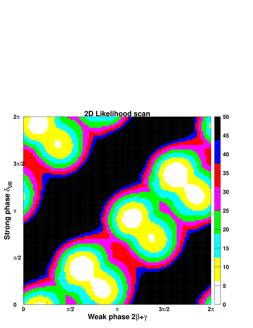
Figure 2: $\chi^{2}$ as a function of $2\beta+\gamma$ and $\delta{{}_{\cal U}}_{0}$, with the parameters of Table 1.

In Fig. 3 we show the one-dimensional minimum projection $\chi^{2}(2\beta+\gamma)=\min\{\chi^{2}(2\beta+\gamma,\delta{{}_{\cal U}}_{0})\}$, showing the smallest value of $\chi^{2}$ for each value of $2\beta+\gamma$.

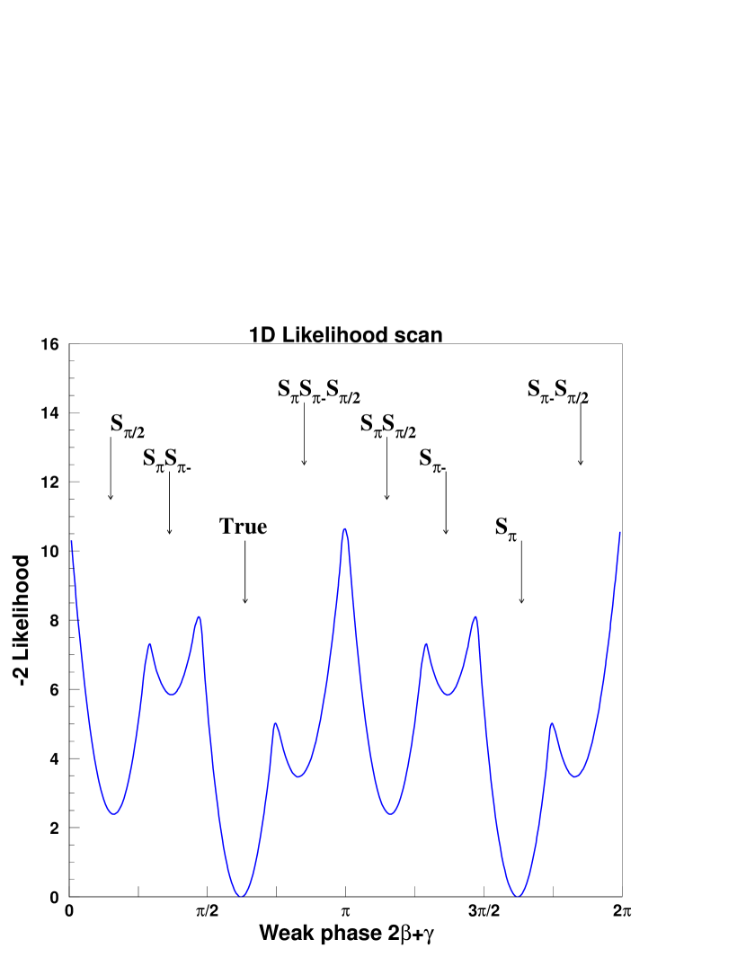
Figure 3: Minimum projection of $\chi^{2}$ onto $2\beta+\gamma$.

With equal resonant and non-resonant $\overline{b}\rightarrow\overline{c}u\overline{s}$ amplitudes, the ambiguities originating from the non-resonant regime are dominant, due to the relative suppression of the resonant interference terms, as they overlap only little with the non-resonant amplitudes. These are however significant enough to resolve all but the $S_{\pi}$ ambiguity.

Figure 4: The error on $2\beta+\gamma$, $\sigma_{2\beta+\gamma}$, as a function of (top) $\widetilde{2\beta\!+\!\gamma}$ and (bottom) $\tilde{A}{{}_{\cal U}}_{0}/\tilde{A}{{}_{\cal C}}_{0}$.

Mode	$N_{ev}$	Mode	$N_{ev}$
$B^{0}\rightarrow D^{-}K^{0}_{s}\pi^{+}$	112	$B^{0}\rightarrow D^{+}K^{0}_{s}\pi^{-}$	33
$\overline{B}\rule{0.0pt}{4.30554pt}^{0}\rightarrow D^{+}K^{0}_{s}\pi^{-}$	111	$\overline{B}\rule{0.0pt}{4.30554pt}^{0}\rightarrow D^{-}K^{0}_{s}\pi^{+}$	33

Table 2: The numbers of perfectly tagged events of each type expected in 400 $\mbox{fb}^{-1}$ obtained by averaging 100 simulations using the parameters of Table 1 and the reconstruction efficiencies listed in the text.

In Fig. 4 we present $\sigma_{2\beta+\gamma}$, the statistical error on $2\beta+\gamma$ as a function of $\widetilde{2\beta\!+\!\gamma}$ and $\tilde{A}{{}_{\cal U}}_{0}/\tilde{A}{{}_{\cal C}}_{0}$, obtained by fitting simulated event samples. Each point is obtained by repeating the simulation 250 times, to minimize sample-to-sample statistical fluctuations. All the parameters of Table 1 were determined by the fit, and the arrow in these figures indicates the point corresponding to the parameters of Table 1. One observes that $\sigma_{2\beta+\gamma}$ does not depend strongly on the value $2\beta+\gamma$. As expected, a strong dependence on $\tilde{A}{{}_{\cal U}}_{0}/\tilde{A}{{}_{\cal C}}_{0}$ is seen. However, it should be noted that $\sigma_{2\beta+\gamma}$ changes very little for all values of $\tilde{A}{{}_{\cal U}}_{0}/\tilde{A}{{}_{\cal C}}_{0}$ above 0.4. This suggests that the potential for a significantly sensitive measurement is high over a broad range of parameters.

5 Conclusions

We have shown how $2\beta+\gamma$ may be measured in the color-allowed decays $B^{0}\rightarrow D^{(*)\mp}K^{(*)0}\pi/\rho^{\pm}$, focusing on the simplest mode $B^{0}\to D^{\pm}K^{0}_{s}\pi^{\mp}$. The absence of color suppression in the $\overline{b}\rightarrow\overline{u}c\overline{s}$ amplitudes is expected to result in relatively large rates and significant CP violation effects, and hence favorable experimental sensitivities. While the Dalitz plot analysis implies some experimental complication, it should reduce the eight-fold ambiguities, which are a serious problem with other methods for measuring $2\beta+\gamma$. As a result of these advantages, this method is likely to lead to a measurement of $2\beta+\gamma$ even with the current generation of $B$ factory experiments.

6 Acknowledgments

The authors thank Francois Le Diberder for his fruitful ideas and help with simulation. This work was supported by CEA and the Danish Research Academy.

References

- [1] BaBar Collaboration (B. Aubert et al.), Phys. Rev. Lett. 86 (2001), 2515.
- [2] Belle Collaboration (B. Abe et al.), Phys. Rev. Lett. 87 (2001), 091802.
- [3] R. Aleksan, T. Petersen and A. Soffer, Phys. Rev. D. 67 (2003) 096002.
- [4] R. Aleksan, B. Kayser and D. London, Phys. Rev. Lett. 73, (1994) 18.
- [5] L. Wolfenstein, Phys. Rev. Lett. 51 (1983) 1945.
- [6] R. Aleksan, I. Dunietz, B. Kayser, F. Le Diberder, Nucl. Phys. B361 (1991) 141.
- [7] The CLEO Collaboration, Phys. Rev. Lett. 88, 101803 (2002).