Flavor Hierarchy from Extra Dimension and Gauge Threshold Correction

Abstract

Dynamical quasi-localization of matter fields in extra dimension is an elegant mechanism to generate hierarchical 4-dimensional Yukawa couplings. We point out that a bulk matter field whose zero mode is quasi-localized can give a large Kaluza-Klein threshold correction to low energy gauge couplings, which is generically of the order of $\ln(\mbox{Yukawa})/8\pi^{2}$, so it can significantly affect gauge coupling unification. We compute such threshold corrections in generic 5-dimensional theories compactified on $S^{1}/Z_{2}\times Z_{2}$, and apply the result to grand unified theories on orbifold generating small Yukawa couplings through quasi-localization.

I Introduction

It has been noticed that extra dimension can provide an elegant mechanism to generate hierarchical Yukawa couplings Arkani-Hamed:1999dc ; Mirabelli:1999ks ; Dvali:2000ha ; Kaplan:2000av ; Arkani-Hamed:2001tb ; Kaplan:2001ga ; Kakizaki:2001ue ; Haba:2002uw ; Hebecker:2002re ; Grossman:2002pb ; Chang:2002ww ; Kitano:2003cn ; Choi:2003di ; Biggio:2003kp . The quark and lepton fields can be quasi-localized in extra dimension in a natural manner, and then their 4-dimensional (4D) Yukawa couplings are determined by the wavefunction overlap factor $e^{-M\pi R}$ where $M$ is a combination of mass parameters in higher dimensional theory and $R$ is the length of extra dimension. This allows that hierarchical Yukawa couplings are obtained from fundamental mass parameters having the same order of magnitude. Extra dimension has been known to be useful also for constructing a natural model of gauge unification Kawamura:2000ev ; Altarelli:2001qj ; Hall:2001pg ; Hebecker:2001wq ; Hebecker:2001jb ; Hall:2001tn ; Asaka:2001eh ; Hall:2001xr ; Dermisek:2001hp ; Kim:2002ab ; Kim:2002im . Supersymmetric 4D grand unified theories (GUTs) successfully accomodate gauge coupling unification, however suffer from some difficulties such as the doublet-triplet splitting problem and the proton decay problem. These problems can be elegantly solved in GUT on orbifold with gauge symmetry broken by boundary conditions Kawamura:2000ev ; Hebecker:2001wq . It is straightforward to implement the idea of dynamical quasi-localization in orbifold GUT to get hierarchical Yukawa couplings as well as successful gauge unification Kakizaki:2001ue ; Hebecker:2002re .

In any GUT, heavy particle threshold effects at GUT symmetry breaking scale should be taken into account for a precision analysis of low energy gauge couplings $g_{a}^{2}$. In conventional 4D GUT, those threshold corrections to $1/g_{a}^{2}$ are generically of the order of $1/8\pi^{2}$ and thus not so important, unless the model contains a large number of superheavy particles which become massive as a consequence of GUT symmetry breaking or some of superheavy masses are hierarchically different from each other Weinberg:1980wa . As was pointed out a long time ago, higher dimensional field theory and/or string theory contain (infinitely) many Kaluza-Klein (KK) or stringy modes, so can have a sizable threshold correction Choi:1987iu . Therefore it is essential to include stringy and/or KK threshold correction in the precision analysis of low energy couplings in string and/or higher dimensional field theories. In this paper, we wish to examine the KK threshold corrections in generic 5D orbifold field theories in which hierarchical 4D Yukawa couplings are generated through quasi-localization. As we will see, the KK threshold corrections to $1/g_{a}^{2}$ in such models are generically of the order of $\ln(\mbox{Yukawa})/8\pi^{2}$, so can significantly affect gauge coupling unification. The outline of this paper is as follows. In Sec. II, we discuss the KK spectrum and zero mode wave functions of generic scalar and spinor fields in 5D theory compactified on $S^{1}/Z_{2}\times Z^{\prime}_{2}$. In Sec. III, we discuss the 4D Yukawa couplings of those quasi-localized scalar and fermion zero modes. In Sec. IV, we compute KK threshold corrections in generic 5D theories on $S^{1}/Z_{2}\times Z^{\prime}_{2}$. In Sec. V, we use these results to derive the KK correction to the predicted value of the low energy QCD coupling constant in 5D GUT on orbifold. We then construct a class of supersymmetric 5D orbifold GUTs which generate hierarchical Yukawa couplings through dynamical quasi-localization while keeping successful gauge coupling unification. Sec. VI is the conclusion.

II Kaluza-Klein analysis and quasi-localized zero modes

In this section, we analyze the KK wave functions and spectrums of scalar and spinor fields in 5D theory compactified on $S^{1}/Z_{2}\times Z^{\prime}_{2}$. Our major concern is the dynamical quasi-localization of zero mode wavefunctions which would result in hierarchical 4D Yukawa couplings. We also consider the full KK spectrums which will be relevant for the discussion of KK threshold corrections to low energy gauge couplings. Throughout this paper, we will use the convention for $S^{1}/Z_{2}\times Z_{2}^{\prime}$ which is given by the following transformation of the fifth spacetime coordinate $y\equiv y+4\pi R$:

$$Z_{2}:y\rightarrow-y\,,\quad\quad Z_{2}^{\prime}:y+\pi R\rightarrow-y+\pi R\,.$$ (1)

so the fundamental domain of $S^{1}/Z_{2}\times Z_{2}^{\prime}$ corresponds to $0\leq y\leq\pi R$.

Let us first consider a 5D complex scalar field with an action:

$$-\int d^{5}x\,\left[\,D_{M}\phi^{zz^{\prime}}D^{M}\phi^{zz^{\prime}*}+\left(\,m_{zz^{\prime}}^{2}+2\mu_{zz^{\prime}}\delta(y)-2\mu_{zz^{\prime}}^{\prime}\delta(y-\pi R)\,\right)\phi^{zz^{\prime}}\phi^{zz^{\prime}*}\,\right]\,,$$ (2)

and the orbifold boundary conditions:

$$\phi^{zz^{\prime}}(-y)=z\phi^{zz^{\prime}}(y)\,,$$

$$\phi^{zz^{\prime}}(-y+\pi R)=z^{\prime}\phi^{zz^{\prime}}(y+\pi R)\,,$$

where $z=\pm 1$ and $z^{\prime}=\pm 1$. The equation of motion for each KK mode of this scalar field is given by

$$\left(\partial_{y}^{2}+(\omega_{n}^{zz^{\prime}})^{2}\right)\phi^{zz^{\prime}}_{n}=2\left[\,\mu_{zz^{\prime}}\delta(y)-\mu^{\prime}_{zz^{\prime}}\delta(y-\pi R)\,\right]\phi^{zz^{\prime}}_{n}\,,$$ (3)

where

$$\left(\omega_{n}^{zz^{\prime}}\right)^{2}=\left(M^{zz^{\prime}}_{n}\right)^{2}-m^{2}_{zz^{\prime}}$$ (4)

for $M_{n}^{zz^{\prime}}$ denoting the 4D mass of $\phi^{zz^{\prime}}_{n}$. Upon ignoring unimportant normalization factor, one easily finds the following KK wave functions on the fundamental domain:

$$\phi^{++}_{n}=\cos\left(\omega_{n}^{++}y\right)+\frac{\mu_{++}}{\omega^{++}_{n}}\sin\left(\omega^{++}_{n}y\right)\,,$$

$$\phi^{+-}_{n}=\sin\left(\omega_{n}^{+-}(y-\pi R)\right)\,,$$

$$\phi^{-+}_{n}=\sin\left(\omega_{n}^{-+}y\right)\,,$$

$$\phi^{--}_{n}=\sin\left(\omega_{n}^{--}y\right)\,,$$ (5)

where $\omega_{n}^{zz^{\prime}}(\neq 0)$ are either real or pure imaginary constants determined by

$$\tan\left(\omega_{n}^{++}\pi R\right) = \frac{(\mu_{++}-\mu^{\prime}_{++})\omega_{n}^{++}}{\left(\omega^{++}_{n}\right)^{2}+\mu_{++}\mu_{++}^{\prime}}\,,$$

$$\tan\left(\omega_{n}^{+-}\pi R\right) = -\frac{\omega^{+-}_{n}}{\mu_{+-}}\,,$$

$$\tan\left(\omega_{n}^{-+}\pi R\right) = \frac{\omega^{-+}_{n}}{\mu^{\prime}_{-+}}\,,$$

$$\tan\left(\omega_{n}^{--}\pi R\right) = 0.$$ (6)

Once $\omega_{n}^{zz^{\prime}}$ are determined, the KK mass spectrum of $\phi^{zz^{\prime}}$ can be determined by the relation

$$\left(M_{n}^{zz^{\prime}}\right)^{2}=m^{2}_{zz^{\prime}}+\left(\omega_{n}^{zz^{\prime}}\right)^{2}.$$ (7)

Note that a pure imaginary $\omega^{zz^{\prime}}_{n}$ gives $\left(M_{n}^{zz^{\prime}}\right)^{2}$ smaller than $m_{zz^{\prime}}^{2}$, while a real $\omega_{n}^{zz^{\prime}}$ gives $\left(M_{n}^{zz^{\prime}}\right)^{2}$ bigger than $m^{2}_{zz^{\prime}}$. Note also that there can be only one or no imaginary $\omega^{zz^{\prime}}_{n}$ from (6).

Since we are interested in the shape of zero mode wavefunction, let us consider the conditions for $\phi^{zz^{\prime}}$ to have a zero mode, i.e $M^{zz^{\prime}}_{0}=0$, independently of the value of the orbifold radius $R$. Obviously only $\phi^{++}$ can have such a zero mode only when its bulk and brane masses are tuned to satisfy

$$\mu_{++}=\mu^{\prime}_{++}\,,\quad m^{2}_{++}=\mu^{2}_{++}\,,$$ (8)

which are indeed satisfied in supersymmetric theories Arkani-Hamed:2001tb ; Gherghetta:2000qt . The resulting zero mode (on the fundamental domain) is given by

$$\phi^{++}_{0}=\exp(\mu_{++}y)\,,$$ (9)

so it is quasi-localized at $y=0$  if  $\mu_{++}<0$, while at $y=\pi R$   if  $\mu_{++}>0$. In a more general case with $\mu_{++}=\mu^{\prime}_{++}$ but $m^{2}_{++}\neq\mu_{++}^{2}$, the KK spectrums of $\phi^{++}$ are given by

$$\left(M^{++}_{0}\right)^{2}=m^{2}_{++}-\mu^{2}_{++}\,,$$

$$\left(M^{++}_{n}\right)^{2}=m^{2}_{++}+\frac{n^{2}}{R^{2}}\,,$$ (10)

for $n$ being a positive integer.

For $\phi^{+-}$,  if  $\mu_{+-}\pi R<-1$, there can be a mode lighter than $m_{+-}$:

$$\phi^{+-}_{0}=\sinh\xi(y-\pi R)\,,$$

$$\left(M^{+-}_{0}\right)^{2}=m_{+-}^{2}-\xi^{2}\,,$$ (11)

where $\xi$ is a real constant determined by

$$\tanh(\xi\pi R)=\frac{\xi}{|\mu_{+-}|}\,.$$

In the limit $\mu_{+-}\pi R\ll-1$,  $M^{+-}_{0}$ is determined to be

$$\left(M_{0}^{+-}\right)^{2}=\left(m^{2}_{+-}-\mu^{2}_{+-}\right)+4\mu^{2}_{+-}\left(e^{-2|\mu_{+-}|\pi R}+{\cal O}(e^{-4|\mu_{+-}|\pi R})\right).$$ (12)

So in supersymmetric case in which $m^{2}_{+-}=\mu^{2}_{+-}$, the mass of $\phi^{+-}_{0}$ is exponentially suppressed in the limit $\mu_{+-}\pi R\ll-1$. On the other hand, all other KK modes of $\phi^{+-}$ are heavier than $m_{+-}$. Similarly,   if   $\mu_{-+}\pi R>1$, $\phi^{-+}$ can have a lighter mode:

$$\phi^{-+}_{0}=\sinh(\xi^{\prime}y)\,,$$

$$\left(M^{-+}_{0}\right)^{2}=m_{-+}^{2}-\xi^{\prime 2}\,,$$

where

$$\tanh(\xi^{\prime}\pi R)=\frac{\xi^{\prime}}{\mu_{-+}}.$$

In the limit $\mu_{-+}\pi R\gg 1$, we have

$$\left(M^{-+}_{0}\right)^{2}=\left(m^{2}_{-+}-\mu^{2}_{-+}\right)^{2}+4\mu^{2}_{-+}\left(e^{-2\mu_{-+}\pi R}+{\cal O}(e^{-4\mu_{-+}\pi R})\right),$$

yielding an exponentially small mass of $\phi^{-+}_{0}$ in supersymmetric case with $\mu_{-+}\pi R\gg 1$.

Let us now consider a 5D spinor field with an action

$$-\int d^{5}x\,\left[\,i\bar{\Psi}^{zz^{\prime}}\left(\gamma^{M}\partial_{M}+{\cal M}_{zz^{\prime}}\epsilon(y)\right)\Psi^{zz^{\prime}}\,\right]\,,$$ (13)

and the orbifold boundary condition

$$\Psi^{zz^{\prime}}(-y) = z\gamma_{5}\Psi^{zz^{\prime}}(y)\,,$$

$$\Psi^{zz^{\prime}}(-y+\pi R) = z^{\prime}\gamma_{5}\Psi^{zz^{\prime}}(y+\pi R)\,,$$

where $\epsilon(y)=-\epsilon(-y)=\epsilon(y+2\pi R)=1$ on the covering space of $S^{1}/Z_{2}\times Z^{\prime}_{2}$. Note that in order for the action to be invariant under $Z_{2}\times Z^{\prime}_{2}$, 5D spinor can have only a kink type mass ${\cal M}_{zz^{\prime}}\epsilon(y)$. The equation of motion for each KK mode of $\Psi^{zz^{\prime}}$ is given by

$$\left(\partial_{y}^{2}+(\omega_{n}^{zz^{\prime}})^{2}\right)^{2}\Psi^{zz^{\prime}}_{nL}=-2{\cal M}_{zz^{\prime}}\left[\,\delta(y)-\delta(y-\pi R)\,\right]\Psi^{zz^{\prime}}_{nL}\,,$$

$$\left(\partial_{y}^{2}+(\omega_{n}^{zz^{\prime}})^{2}\right)^{2}\Psi^{zz^{\prime}}_{nR}=+2{\cal M}_{zz^{\prime}}\left[\,\delta(y)-\delta(y-\pi R)\,\right]\Psi^{zz^{\prime}}_{nR},$$ (14)

where $\gamma_{5}\Psi_{L,R}=\pm\Psi_{L,R}$ and

$$\left(\omega_{n}^{zz^{\prime}}\right)^{2}=\left(M_{n}^{zz\prime}\right)^{2}-\left({\cal M}^{zz^{\prime}}\right)^{2}$$

for $M^{zz^{\prime}}_{n}$ denoting the 4D mass of $\Psi_{n}^{zz^{\prime}}$. When compared to the scalar equation of motion (3), this suggests that in supersymmetric case the bulk and brane scalar masses should satisfy

$$\mu_{zz^{\prime}}=\mu^{\prime}_{zz^{\prime}},\quad\mu^{2}_{zz^{\prime}}=m_{zz^{\prime}}^{2}={\cal M}_{zz^{\prime}}^{2}.$$

Obviously, $\Psi^{++}$ has a left-handed zero mode for any value of ${\cal M}_{++}$:

$$\Psi^{++}_{0L}(y)=\exp(-{\cal M}_{++}y)$$ (15)

which is quasi-localized at either $y=0$ (if ${\cal M}_{++}>0$) or $y=\pi R$ (if ${\cal M}_{++}<0$). All other left-handed modes of $\Psi^{++}$ are paired-up with right-handed modes to get a 4D Dirac mass bigger than ${\cal M}_{++}$:

$$M^{++}_{n}=\sqrt{{\cal M}_{++}^{2}+\frac{n^{2}}{R^{2}}}\,.$$ (16)

Similarly, $\Psi^{--}$ has a right-handed zero mode for any value of ${\cal M}_{--}$ and also the massive modes with $(M_{n}^{--})^{2}={\cal M}^{2}_{--}+n^{2}/R^{2}$. The wave function of zero mode is given by

$$\Psi^{--}_{0R}(y)=\exp({\cal M}_{--}y),$$ (17)

so the zero mode is quasi-localized at either $y=0$ (if ${\cal M}_{--}<0$) or $y=\pi R$ (if ${\cal M}_{--}>0$).

For $\Psi^{+-}$, there is no zero mode. However if ${\cal M}_{+-}\pi R>1$, there can be two modes lighter than ${\cal M}_{+-}$, while all other modes are heavier than ${\cal M}_{+-}$ The wavefunctions of light modes are given by

$$\Psi^{+-}_{0L}(y) = \sinh(k(y-\pi R)),$$ (18)

$$\Psi^{+-}_{0R}(y) = \sinh(ky),$$ (19)

where $k$ is a real constant determined by

$$\tanh({k\pi R})=\frac{k}{{\cal M}_{+-}}.$$ (21)

Obviously, one of these two light modes is localized at $y=0$, while the other is localized at $y=\pi R$. In 4D viewpoint, these two modes are paired up to get a Dirac mass

$$\left(M^{+-}_{0}\right)^{2}={\cal M}_{+-}^{2}-k^{2}\,.$$ (22)

Note that in the limit ${\cal M}_{+-}\pi R\gg 1$,

$$M^{+-}_{0}\approx 2{\cal M}_{+-}\exp(-{\cal M}_{+-}\pi R),$$ (23)

so $\Psi^{+-}_{0}$ can be arbitrarily light. Similarly, if ${\cal M}_{-+}\pi R<-1$, $\Psi^{-+}$ can have a light Dirac mode with $M^{-+}_{0}\approx 2|{\cal M}_{-+}|\exp({\cal M}_{-+}\pi R)$.

The dynamical quasi-localization of light modes and also the shape of full KK spectrums offer a possibility that massless brane fields can be considered as a large mass limit of bulk fields . To see this, let us take the limit $|{\cal M}_{zz^{\prime}}|\to\infty$ . In this limit, the left-handed zero mode of $\Psi^{++}$ becomes a chiral brane fermion confined at $y=0$ (if ${\cal M}_{++}\rightarrow\infty$) or at $y=\pi R$ (if ${\cal M}_{++}\rightarrow-\infty$), while the right-handed zero mode of $\Psi^{--}$ becomes a chiral brane fermion at $y=0$ (if ${\cal M}_{--}\rightarrow-\infty$) or at $y=\pi R$ (if ${\cal M}_{--}\rightarrow\infty$). For $\Psi^{+-}$, the light modes $\Psi^{+-}_{0L}$ and $\Psi^{+-}_{0R}$ become a massless brane fermion at $y=0$ and $y=\pi R$, respectively, in the limit ${\cal M}_{+-}\rightarrow\infty$. Similarly, $\Psi^{-+}_{0L}$ and $\Psi^{-+}_{0R}$ become a massless brane fermion at $y=\pi R$ and $y=0$, respectively, in the limit ${\cal M}_{-+}\rightarrow-\infty$. All other KK modes of $\Psi^{zz^{\prime}}$ are heavier than $|{\cal M}_{zz^{\prime}}|$, and thus are decoupled in the limit $|{\cal M}_{zz^{\prime}}|\rightarrow\infty$. So any massless brane fermion can be considered as a bulk fermion in the large kink mass limit.

III Yukawa hierarchy from quasi-localization

To discuss flavor hierarchy arising from quasi-localization, let us consider a generic 5D theory containing arbitrary number of scalar and fermion fields:

$$S = -\int d^{5}x\left[\,D_{M}\phi_{I}D^{M}\phi^{*}_{I}+\left(m_{I}^{2}\delta_{IJ}+2\mu_{IJ}\delta(y)-2\mu^{\prime}_{IJ}\delta(y-\pi R)\right)\phi_{I}\phi^{*}_{J}\right.$$ (24)

$$\left.\quad\quad\quad\quad+\,i\bar{\Psi}_{A}(\gamma^{M}D_{M}+{\cal M}_{A}\epsilon(y))\Psi_{A}+{\cal L}_{Y}\,\right]\,.$$

Here ${\cal L}_{Y}$ stands for the Yukawa couplings between $\phi_{I}$ and $\Psi_{A}$ and the orbifold boundary conditions are given by

$$\phi_{I}(-y)=z_{I}\phi(y), \,\,\phi_{I}(-y+\pi R)=z_{I}^{\prime}\phi_{I}(y+\pi R)\,,$$

$$\Psi_{A}(-y)=z_{A}\gamma_{5}\Psi_{A}(y), \,\,\Psi_{A}(-y+\pi R)=z_{A}^{\prime}\gamma_{5}\Psi_{A}(y+\pi R)\,.$$ (25)

Though the brane masses of scalar fields can have off-diagonal components in general, we will assume for simplicity that they are diagonal: $\mu_{IJ}=\mu_{I}\delta_{IJ}$ and $\mu^{\prime}_{IJ}=\mu^{\prime}_{I}\delta_{IJ}$. To get hierarchical 4D Yukawa couplings, we also assume that Yukawa couplings in 5D theory exist only at the fixed points, which is assured by 5D SUSY in supersymmetric theories. Then the most general form of Yukawa couplings can be written as

$${\cal L}_{Y}=\delta(y)\,\frac{{\lambda}_{{}_{XPQ}}}{\Lambda^{3/2}}\,\varphi_{{}_{X}}\psi_{{}_{P}}\psi_{{}_{Q}}+\delta(y-\pi R)\,\frac{{\lambda}^{\prime}_{{}_{XPQ}}}{\Lambda^{3/2}}\,\varphi_{{}_{X}}\psi_{{}_{P}}\psi_{{}_{Q}}+{c.c.},$$ (26)

where $\Lambda$ denotes the cutoff scale of our 5D orbifold field theory, $\varphi_{{}_{X}}=\{\phi_{I}\,\,\,\mbox{or}\,\,\,\phi^{*}_{I}\}$, and $\psi_{{}_{P}}=\{\frac{1}{2}(1+\gamma_{5})\Psi_{A}\,\,\mbox{or}\,\,\frac{1}{2}(1+\gamma_{5})\Psi_{A}^{c}\}$. Note that $\lambda_{ipq}$ and $\lambda^{\prime}_{ipq}$ are dimensionless parameters in our convention.

Let $\phi_{i}$ denote 5D scalar fields having a zero mode $\phi_{0i}=\exp(m_{i}y)$, i.e. scalar fields with $z_{i}=z^{\prime}_{i}=1$ and $\mu_{i}=\mu^{\prime}_{i}=m_{i}$, and $\Psi_{p}$ denote 5D spinor fields having a chiral zero mode $\psi_{0p}=\exp(-z_{p}{\cal M}_{p}y)$, i.e. spinor fields with $z_{p}=z^{\prime}_{p}=\pm 1$. It is then straightforward to find that the 4D Yukawa couplings of canonocally normalized zero modes are given by

$$y_{ipq} = \sqrt{Z(m_{i})Z(-z_{p}{\cal M}_{p})Z(-z_{q}{\cal M}_{q})}\,\,\lambda_{ipq}$$ (27)

$$+\sqrt{Z(-m_{i})Z(z_{p}{\cal M}_{p})Z(z_{q}{\cal M}_{q})}\,\,\lambda^{\prime}_{ipq}$$

where

$$Z(m)=\frac{2m}{\Lambda}\frac{1}{e^{2m\pi R}-1}.$$ (28)

Obviously, $y_{ipq}$ can have very different values, depending upon the values of $m_{i}$ and ${\cal M}_{p,q}$, even when all of the 5D parameters $\lambda_{ipq}$ and $\lambda^{\prime}_{ipq}$ have similar values.

A simple way to get hierarchical Yukawa couplings through quasi-localization is to assume that all Yukawa couplings originate from a single fixed point, for instance from $y=\pi R$. As a concrete example, let us consider the case that all Yukawa couplings originate from $y=\pi R$ and $\phi_{i}$ is a brane field confined at $y=\pi R$ with $Z(-m_{i})\approx 1$. Note that a brane scalar field at $y=\pi R$ can be obtained from a bulk scalar field by taking the limit $m={\cal O}(\Lambda)$ while keeping $\mu=\mu^{\prime}=m$. Then for $z_{p,q}{\cal M}_{p,q}\lesssim-1/R$, we have

$$y_{ipq}\approx\sqrt{\frac{4|{\cal M}_{p}{\cal M}_{q}|}{\Lambda^{2}}}\,\,{\lambda}^{\prime}_{ipq}\,,$$ (29)

while for $z_{p,q}{\cal M}_{p,q}\gtrsim 1/R$,

$$y_{ipq}\approx\sqrt{\frac{4|{\cal M}_{p}{\cal M}_{q}|}{\Lambda^{2}}}\,e^{-(z_{p}{\cal M}_{p}+z_{q}{\cal M}_{q})\pi R}\,\,{\lambda}^{\prime}_{ipq}.$$ (30)

The physical interpretation of this result is simple. If $z_{p,q}{\cal M}_{p,q}\gtrsim 1/R$, the corresponding zero modes are quasi-localized at $y=0$, so the Yukawa couplings are exponentially suppressed as they originate from $y=\pi R$. On the other hand, for $z_{p,q}{\cal M}_{p,q}\lesssim-1/R$, the zero modes are localized at $y=\pi R$, so there is no exponential suppression in Yukawa couplings.

If the fundamental theory at $\Lambda$ is weakly coupled, simple dimensional analysis would suggest that the dimensionless ${\lambda}_{ipq}$ are of order unity or less. However a more interesting possibility is that the theory is strongly coupled at $\Lambda$ Chacko:1999hg ; Nomura:2001tn . In 5D theories under consideration, the standard model gauge fields live in bulk spacetime, so their 4D couplings are given by $1/{g_{a}^{2}}\approx{\pi R}/{g_{5a}^{2}}$, where $g^{2}_{5a}$ denote the dimensionful 5D gauge couplings with mass dimension $-1$. In order for our 5D theory to be a useful framework, it must be valid up to an energy scale significantly higher than the compactification scale $1/R$, i.e. $\Lambda\gg 1/R$. If $\Lambda$ were comparable to $1/R$, we would not have to consider a 5D theory as an intermediate step going from the fundamental theory at $\Lambda$ to the 4D effective theory for low energy physics. We would rather go directly to the 4D effective theory from the fundamental theory. On the other hand, if $\Lambda\gg 1/R$ as desired, we have $g_{5a}^{2}\approx\pi Rg_{a}^{2}\gg{1}/{\Lambda}$, implying that the fundamental theory at $\Lambda$ is strongly coupled. As is well known, only in strongly coupled scenario, GUT on orbifold can provide a meaningful prediction for $\sin^{2}\theta_{W}$ or the QCD coupling constant at the weak scale. In such strongly-coupled scenario, dimensional analysis suggests

$${\lambda}^{\prime}_{ipq}={\cal O}(4\pi).$$

It is then straightforward to get hierarchical 4D Yukawa couplings ranging from the top quark Yukawa coupling $y_{t}\approx 1$ to the electron Yukawa coupling $y_{e}\approx 10^{-5}-10^{-6}$ within the parameter range

$$\Lambda\pi R={\cal O}(10^{2})\,,\quad|{\cal M}_{p}|\pi R\lesssim 7\,.$$

Note that, in strongly coupled scenario, if the Higgs boson and the left and right-handed top quarks are all brane fields, the resulting top-quark Yukawa coupling would be too large, $y_{t}={\cal O}(4\pi)$, so one needs to put some of those fields in bulk spacetime.

In supersymmetric 5D theories, the fermion kink masses ${\cal M}_{p}$ are related to the graviphoton gauging Ceresole:2000jd ; Choi:2002wx :

$$D_{M}\Psi_{p}=\partial_{M}\Psi_{p}+i{\cal M}_{p}\epsilon(y)B_{M}\Psi_{p}+...\,,$$ (31)

where $B_{M}$ denotes the graviphoton. This suggests that it is a plausible assumption that ${\cal M}_{p}$ are quantized (in an appropriate unit) as the conventional gauge charges are quantized. If true, the resulting Yukawa couplings (30) would have the same form as those obtained from the Frogatt-Nielson mechanism which generates small Yukawa couplings using a spontaneously broken $U(1)$ flavor symmetry Froggatt:1978nt . In the next section, we will see that the KK threshold corrections to low energy gauge couplings are generically given by

$$\Delta\left(\frac{1}{g_{a}^{2}}\right)={\cal O}\left(\frac{\ln(y_{ipq})}{8\pi^{2}}\right),$$ (32)

if the hierarchical 4D Yukawa couplings $y_{ipq}$ are generated by quasi-localization. Obviously then the KK threshold corrections can significantly affect the gauge coupling unification.

IV kaluza-klein threshold correction to low energy gauge coupling

In this section, we discuss the 1-loop threshold correction to low energy gauge coupling in 5D orbifold field theory. The bare action of bulk gauge fields can be written as

$$S_{\rm bare}=-\int d^{5}x\left(\frac{1}{4g_{5a}^{2}}+\frac{\kappa_{a}}{4}\delta(y)+\frac{\kappa^{\prime}_{a}}{4}\delta(y-\pi R)\right)F^{aMN}F^{a}_{MN},$$ (33)

and then the 4D gauge couplings at tree level are given by

$$\left(\frac{1}{g_{a}^{2}}\right)_{\rm tree}=\frac{\pi R}{g_{5a}^{2}}+\kappa_{a}+\kappa^{\prime}_{a}.$$ (34)

One-loop corrections to low energy couplings can be computed by summing the contributions from all KK modes. In generic 5D orbifold field theory, such computation yields Contino:2001si ; Choi:2002zi

$$\frac{1}{g_{a}^{2}(p)} = \left[\frac{\pi R}{g_{5a}^{2}}+\frac{\gamma_{a}}{24\pi^{3}}\Lambda\pi R+\kappa_{a}+\kappa^{\prime}_{a}\right]+\frac{1}{8\pi^{2}}\left[{\Delta}_{a}(\ln\Lambda,m,\mu,\mu^{\prime},{\cal M},R)+b_{a}\ln\left(\frac{\Lambda}{p}\right)\right]\,$$ (35)

$$\equiv \left(\frac{1}{g_{a}^{2}}\right)_{\rm bare}+\frac{1}{8\pi^{2}}\left[\Delta_{a}(\ln\Lambda,m,\mu,\mu^{\prime},{\cal M},R)+b_{a}\ln\left(\frac{\Lambda}{p}\right)\right]$$

where $\gamma_{a}$ are the coefficients of (UV-sensitive) linearly divergent corrections, $\Delta_{a}$ stand for (UV-insensitive) logarithmically divergent or finite threshold corrections due to massive KK modes, and $b_{a}$ are the standard 1-loop beta function coefficients due to zero modes. Here $(1/g_{a}^{2})_{\rm bare}$ correspond to the uncalculable bare couplings of the model, while $\Delta_{a}$ are unambiguously calculable within 5D orbifold field theory. Note that $\Delta_{a}$ contain a piece linear in $\ln\Lambda$ as well as a finite piece depending on the scalar and fermion mass parameters $m,\mu,\mu^{\prime},{\cal M}$ and also on the orbifold radius $R$. Here we assume that the cutoff scale $\Lambda$ is large enough compared to other mass parameters of the theory, thus ignore the part suppressed by an inverse power of $\Lambda$. In the above expression, the renormalization point $p$ is assumed to be below the mass of the lightest massive KK mode, $M_{KK}$, but far above the masses of all zero modes which would be around the weak scale.

The KK threshold corrections in 5D theories on warped $S^{1}/Z_{2}\times Z^{\prime}_{2}$ have been discussed before in Choi:2002wx ; Choi:2002zi ; Choi:2002ps . In Choi:2002wx ; Choi:2002zi , $\Delta_{a}$ for supersymmetric 5D theories on warped $S^{1}/Z_{2}\times Z^{\prime}_{2}$ have been computed in the framework of 4D effective supergravity. In this framework, $\Delta_{a}$ could be obtained by computing the tree-level Kähler potential and also the one-loop correction to holomorphic gauge kinetic functions which can be determined by the chiral anomaly structure of 5D orbifold field theory Arkani-Hamed:2001is . The KK threshold corrections for nonsupersymmetric 5D theories on warped $S^{1}/Z_{2}\times Z^{\prime}_{2}$ have been computed in Choi:2002ps by directly evaluating all KK mode contributions in dimensional regularization scheme GrootNibbelink:2001bx , and it was confirmed that the results in supersymmetric limit agree with those of Choi:2002wx ; Choi:2002zi . In this paper, we compute the KK threshold corrections in generic 5D theories on flat $S^{1}/Z_{2}\times Z_{2}^{\prime}$ with quasi-localized zero modes using the method of Choi:2002ps .

To calculate one-loop gauge couplings at low energies, we integrate out all massive KK modes and derive the one-loop effective action of gauge field zero mode $A_{\mu}$:

$$S_{\rm eff}=S_{\rm bare}+\Gamma_{\phi}+\Gamma_{\Psi}+\Gamma_{A}\,,$$ (36)

where $S_{\rm bare}$ is given in (33), and the 1-loop contributions from 5D scalar $\phi$, 5D spinor $\Psi$ and 5D vector $A_{M}$ are given by

$$i\Gamma_{\phi} \,=\, -\frac{1}{2}{\rm Tr}_{\phi}\ln\,(-D^{2}+M^{2}(\phi))\,,$$

$$i\Gamma_{\Psi} \,=\, \frac{1}{2}{\rm Tr}_{\Psi}\ln\,(-D^{2}+M^{2}(\Psi)+F_{\mu\nu}J^{\mu\nu}_{1/2})+{\rm Tr}_{\Psi_{0}}\ln(\,D\!\!\!\!/\,)\,,$$

$$i\Gamma_{A} \,=\, -\frac{1}{2}{\rm Tr}_{A_{\mu}}\ln\,(-D^{2}+M^{2}(A_{\mu})+F_{\mu\nu}J^{\mu\nu}_{1})-\frac{1}{2}{\rm Tr}_{A_{5}}\ln\,(-D^{2}+M^{2}(A_{5}))$$ (37)

$$+\,{\rm Tr}_{\xi\bar{\xi}}\ln\,(-D^{2}+M^{2}(\xi))\,.$$

Here ${\rm Tr}_{\Phi}$ implies the functional trace for the 5D field $\Phi$, so contains the summations over the whole KK modes. $M^{2}(\Phi)$ denotes the mass-square operator whose eigenvalues correspond to the KK mass spectrum of $\Phi$, and $J^{\mu\nu}_{j}$ is the 4D Lorentz generator for spin $j$, normalized as ${\rm tr}(J_{j}^{\mu\nu}J_{j}^{\rho\sigma})=C(j)(g^{\mu\rho}g^{\nu\sigma}-g^{\mu\sigma}g^{\nu\rho})$ where $C(j)=(0,1,2)$ for $j=(0,1/2,2)$. ${\rm Tr}_{\Psi_{0}}$ denotes the functional trace for the zero mode of $\Psi$ and ${\rm Tr}_{\xi\bar{\xi}}$ is the trace over the ghost fields.

The most convenient way to calculate ${\rm Tr}_{\Phi}$ is to replace the KK summation by a contour integration with an appropriately chosen pole function $P(q)$. The pole function we will use here has the form

$$P(q)=\frac{N^{\prime}(q)}{2N(q)}\,,$$ (38)

where $N(q)$ has zeroes at $q^{2}=M^{2}_{n}(\Phi)-m_{\Phi}^{2}$ for $M_{n}(\Phi)$ denoting the n-th KK mass and $m_{\Phi}$ denoting the bulk mass of $\Phi$. Note that our pole function is different from the pole function of GrootNibbelink:2001bx ; Choi:2002ps as the pole positions are shifted by $m^{2}_{\Phi}$, which is mainly for the simplicity of calculation. Using the analysis of Sec. II, we find the following forms of $N$-functions for 5D scalar and fermion fields:

$$N_{\phi^{++}}(q) = -\frac{1}{q}(q^{2}+\mu_{++}\mu^{\prime}_{++})\sin(q\pi R)+(\mu_{++}-\mu^{\prime}_{++})\cos(q\pi R)\,,$$

$$N_{\phi^{+-}}(q) = \frac{1}{q}(\mu_{+-}\sin(q\pi R)+q\cos(q\pi R))\,,$$

$$N_{\phi^{-+}}(q) = \frac{1}{q}(-\mu^{\prime}_{-+}\sin(q\pi R)+q\cos(q\pi R))\,,$$

$$N_{\phi^{--}}(q) = \frac{1}{q}\sin(q\pi R)\,,$$

$$N_{\Psi^{++}}(q) = \frac{1}{q}\sin(q\pi R)\,,$$

$$N_{\Psi^{+-}}(q) = \frac{1}{q}(-{\cal M}_{+-}\sin(q\pi R)+q\cos(q\pi R))\,,$$

$$N_{\Psi^{-+}}(q) = \frac{1}{q}({\cal M}_{-+}\sin(q\pi R)+q\cos(q\pi R))\,,$$

$$N_{\Psi^{--}}(q) = \frac{1}{q}\sin{q\pi R}\,,$$ (39)

where the scalar and fermion mass parameters $\mu_{zz^{\prime}}$, $\mu^{\prime}_{zz^{\prime}}$ and ${\cal M}_{zz^{\prime}}$ are defined in (2) and (13). The $N$-functions for 5D vector fields $A_{M}^{zz^{\prime}}$ are also easily found to be

$$N_{A^{++}}(q) = \frac{1}{q}\sin(q\pi R)\,,$$

$$N_{A^{+-}}(q) = \cos(q\pi R)\,,$$

$$N_{A^{-+}}(q) = \cos(q\pi R)\,,$$

$$N_{A^{--}}(q) = \frac{1}{q}\sin(q\pi R)\,,$$ (40)

where the boundary conditions of $A^{zz^{\prime}}_{M}$ are given by

$$A^{zz^{\prime}}_{\mu}(-y)=zA^{zz^{\prime}}_{\mu}(y)\,,\quad A^{zz^{\prime}}_{\mu}(-y+\pi R)=z^{\prime}A^{zz^{\prime}}(y+\pi R)\,,$$

$$A^{zz^{\prime}}_{y}(-y)=-zA^{zz^{\prime}}_{y}(y)\,,\quad A^{zz^{\prime}}_{y}(-y+\pi R)=-z^{\prime}A^{zz^{\prime}}_{y}(y+\pi R)\,.$$

Figure 1: Contour $C_{1}$ in the complex q-plane. Bold dots represent poles at $q^{2}=M^{2}_{n}(\Phi)-m^{2}_{\Phi}$ where $M_{n}$ is the KK mass eigenvalue and $m_{\Phi}$ is the bulk mass of 5D field $\Phi$. Note that a 4D state with $M_{n}<m_{\Phi}$ appears as a pole at the imaginary axis.

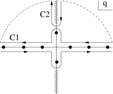
Figure 2: The contour $C_{1}$ on the upper half-plane can be deformed into $C_{2}$ without touching any singularity. The poles at the imaginary axis do not overlap with the brance cut unless there is a tachyon state.

For the pole function defined as above, it is straightforward to find

$${\rm Tr}\ln\,(-D^{2}+M^{2}(\Phi)+F_{\mu\nu}J^{\mu\nu}_{j})$$

$$= \int_{C_{1}}\frac{dq}{2\pi i}\,P(q)\,\int\frac{d^{4}p}{(2\pi)^{4}}A^{a}_{\mu}(-p)A^{a}_{\nu}(p)T_{a}(\Phi)$$

$$\times\left[d(j)\int\frac{d^{4}k}{(2\pi)^{4}}\frac{g^{\mu\nu}\left((p+k)^{2}+q^{2}+m_{\Phi}^{2}\right)-\frac{1}{2}(p+2k)^{\mu}(p+2k)^{\nu}}{\left(k^{2}+q^{2}+m_{\Phi}^{2}\right)\left((p+k)^{2}+q^{2}+m_{\Phi}^{2}\right)}\right.$$

$$\quad\quad\left.-2C(j)\left(p^{2}g^{\mu\nu}-p^{\mu}p^{\nu}\right)\int\frac{d^{4}k}{(2\pi)^{4}}\frac{1}{\left(k^{2}+q^{2}+m_{\Phi}^{2}\right)\left((p+k)^{2}+q^{2}+m_{\Phi}^{2}\right)}\,\right]$$

$$\equiv i\int\frac{d^{4}p}{(2\pi)^{4}}\,{\cal G}_{a}(p)A^{a}_{\mu}(-p)\left(p^{2}g^{\mu\nu}-p^{\mu}p^{\nu}\right)A^{a}_{\nu}(p)\,,$$ (42)

where $d(j)=(1,4,4)$ and $C(j)=(0,1,2)$ for $j=(0,1/2,1)$, and $T_{a}(X)={\rm Tr}\left(T^{2}_{a}(X)\right)$ is the Dynkin index of the gauge group representation $X$. Here the contour $C_{1}$ is depicted in Fig. 1. To regulate the divergent part of the above integral, we split the pole function into two parts:

$$P(q)=\tilde{P}(q)+P_{\infty}(q),$$ (43)

where $\tilde{P}\to O(q^{-2})$ at $|q|\to\infty$. Then $P_{\infty}$ is given by

$$P_{\infty}(q)=-\frac{A}{q}-\frac{i\pi R}{2}\epsilon({\rm Im}(q))\,,$$ (44)

where $\epsilon(x)=x/|x|$ and $A$ is a real constant depending on the $Z_{2}\times Z_{2}^{\prime}$ parity of the corresponding 5D field:

$$A=\left(-1/2,\,0,\,0,\,1/2\right)$$

for $Z_{2}\times Z_{2}^{\prime}$ parity $(Z_{\Phi},Z^{\prime}_{\Phi})=(++,+-,-+,--)$. With the decomposition (43), all UV divergences appear in the contribution from $P_{\infty}$ in a manner allowing simple dimensional regularization.

The 4D momentum integral $d^{4}k$ in (42) exhibits a branch cut on the imaginary axis of $q$ for $p^{2}>0$. For the contribution from $\tilde{P}$, one can change the contour as in Fig. 2 since the contribution from the infinite half-circle vanishes. Note that the poles of $\tilde{P}$ on the imaginary axis do not overlap with the branch cut as long as there is no tachyon. After integrating by part, we find that the part of ${\cal G}_{a}$ from $\tilde{P}$ is given by

$$\Delta{\cal G}_{a}(\tilde{P}) = \frac{T_{a}(\Phi)}{8\pi^{2}}\left(\frac{1}{6}d(j)-2C(j)\right){\cal F}(q)\Big{|}_{q\to i\infty}$$ (45)

$$-\frac{T_{a}(\Phi)}{8\pi^{2}}\int_{0}^{1}dx\left(\frac{1}{2}d(j)(1-2x)^{2}-2C(j)\right){\cal F}(q)\Big{|}_{q=i\sqrt{x(1-x)p^{2}+m_{\Phi}^{2}}}\,,$$

where

$${\cal F}(q)=\frac{1}{2}\ln N+A\ln q+\frac{i\pi R}{2}q\,.$$

In fact, ${\cal F}(q)\Big{|}_{q\to i\infty}$ turns out to be vanishing in the cases we are now considering. The contribution from $P_{\infty}$ includes the log divergence from the pole term $1/q$. This can be regulated by the standard dimensional regularization of 4D momentum integral, $d^{4}p\to d^{D}p$, yielding a $1/(D-4)$ pole. On the other hand, the step-function contribution from $\epsilon({\rm Im}(q))$ involves a 5D momentum integral which is linearly divergent, but it simply gives a finite result in dimensional regularization. Note that linearly divergent correction to $1/g_{a}^{2}$ depends highly on the used regularization scheme. Namely the coefficient $\gamma_{a}$ of Eq. (35) is regularization scheme dependent, and $\gamma_{a}=0$ in the dimensional regularization scheme we are currently using. However this does not have any special meaning since the physical amplitudes are always expressed in terms of the scheme-independent combination $\frac{\pi R}{g_{5a}^{2}}+\frac{\gamma_{a}}{24\pi^{3}}\Lambda\pi R$. Adding the divergent contribution from ${P}_{\infty}$ to the finite part $\Delta{\cal G}_{a}$ from $\tilde{P}$, we obtain

$${\cal G}_{a} = \frac{T_{a}(\Phi)}{8\pi^{2}}\left[\int_{0}^{1}dx\,\left(-\frac{1}{2}d(j)(1-2x)^{2}+2C(j)\right)\left(\frac{1}{2}\ln N\right)\Big{|}_{q=i\sqrt{x(1-x)p^{2}+m_{\Phi}^{2}}}\right.$$ (46)

$$\left.+A\int_{0}^{1}dx\left(-\frac{1}{2}d(j)(1-2x)^{2}+2C(j)\right)\left(\frac{1}{D-4}\right)\right]\,.$$

Using the above result, we find that the KK threshold corrections from a 5D complex scalar $\phi$, 5D Dirac fermion $\Psi$ and 5D vector $A_{M}$ are given by

$$\Delta_{a}(\phi)+b^{\phi}_{a}\ln\frac{\Lambda}{p} = \frac{1}{6}\left[T_{a}(\phi^{++})\left\{\ln\Lambda-3\int_{0}^{1}duF(u)\ln N_{\phi^{++}}\left(i\sqrt{\frac{u^{2}p^{2}}{4}+m_{++}^{2}}\right)\right\}\right.$$

$$\quad\quad-\,3T_{a}(\phi^{+-})\int_{0}^{1}du\,F(u)\ln N_{\phi^{+-}}\left(i\sqrt{\frac{u^{2}p^{2}}{4}+m_{+-}^{2}}\right)$$

$$\quad\quad-\,3T_{a}(\phi^{-+})\int_{0}^{1}du\,F(u)\ln N_{\phi^{-+}}\left(i\sqrt{\frac{u^{2}p^{2}}{4}+m_{-+}^{2}}\right)$$

$$\left.\quad\quad-\,T_{a}(\phi^{--})\left\{\ln\Lambda+3\int_{0}^{1}du\,F(u)\ln N_{\phi^{--}}\left(i\sqrt{\frac{u^{2}p^{2}}{4}+m_{--}^{2}}\right)\right\}\,\right],$$

$$\Delta_{a}(\Psi)+b_{a}^{\Psi}\ln\frac{\Lambda}{p} = \frac{1}{3}\left[T_{a}(\Psi^{++})\left\{-2\ln p+3\int_{0}^{1}du\,G(u)\ln N_{\Psi^{++}}\left(i\sqrt{\frac{u^{2}p^{2}}{4}+{\cal M}_{++}^{2}}\right)\right\}\right.$$

$$\quad\quad+\,T_{a}(\Psi^{+-})\left\{+3\int_{0}^{1}du\,G(u)\ln N_{\Psi^{+-}}\left(i\sqrt{\frac{u^{2}p^{2}}{4}+{\cal M}_{+-}^{2}}\right)\right\}$$

$$\quad\quad+\,T_{a}(\Psi^{-+})\left\{+3\int_{0}^{1}du\,G(u)\ln N_{\Psi^{-+}}\left(i\sqrt{\frac{u^{2}p^{2}}{4}+{\cal M}_{-+}^{2}}\right)\right\}$$

$$\left.\quad\quad+\,T_{a}(\Psi^{--})\left\{-2\ln{p}+3\int_{0}^{1}du\,G(u)\ln N_{\Psi^{--}}\left(i\sqrt{\frac{u^{2}p^{2}}{4}+{\cal M}_{--}^{2}}\right)\right\}\,\right]\,$$

$$\Delta_{a}(A_{M})+b_{a}^{A}\ln\frac{\Lambda}{p} = \frac{1}{12}\left[T_{a}(A^{++}_{M})\left\{-23\ln\Lambda+44\ln p+\int_{0}^{1}du\,K(u)\ln N_{A^{++}}\left(\frac{iu}{2}\sqrt{p^{2}}\right)\right\}\right.$$

$$\quad\quad+\,T_{a}(A^{+-}_{M})\int_{0}^{1}du\,K(u)\ln N_{A^{+-}}\left(\frac{iu}{2}\sqrt{p^{2}}\right)$$

$$\quad\quad+\,T_{a}(A^{-+}_{M})\int_{0}^{1}du\,K(u)\ln N_{A^{-+}}\left(\frac{iu}{2}\sqrt{p^{2}}\right)$$

$$\left.\quad\quad+\,T_{a}(A^{--}_{M})\left\{23\ln\Lambda-2\ln p+\int_{0}^{1}du\,K(u)\ln N_{A^{--}}\left(\frac{iu}{2}\sqrt{p^{2}}\right)\right\}\,\right]\,,$$

where $b_{a}^{\phi}$, $b_{a}^{\psi}$ and $b_{a}^{A}$ are the beta function coefficients for the massless modes from $\phi$, $\Psi$ and $A_{M}$, respectively, and

$$F(u) = u(1-u^{2})^{1/2}\,,$$

$$G(u) = u(1-u^{2})^{1/2}-u(1-u^{2})^{-1/2}\,,$$

$$K(u) = -9u(1-u^{2})^{1/2}+24u(1-u^{2})^{-1/2}\,.$$

For the case that $\sqrt{p^{2}}$ is much smaller than the lowest nonzero KK mass, the above results are simplified to yield

$$\Delta_{a} =\,\frac{21}{12}\left[T_{a}(A^{++}_{M})+T_{a}(A^{--}_{M})\right]\ln(\Lambda\pi R)$$ (47)

$$-\frac{1}{6}T_{a}({\Phi}^{++})\ln\left(\frac{\Lambda(e^{m_{++}\pi R}-e^{-m_{++}\pi R})}{2m_{++}}\right)$$

$$-\frac{1}{6}T_{a}(\phi^{++})\ln\left(\frac{(m_{++}+\mu_{++})(m_{++}-\mu^{\prime}_{++})e^{m_{++}\pi R}-(m_{++}-\mu_{++})(m_{++}+\mu^{\prime}_{++})e^{-m_{++}\pi R}}{2m_{++}\Lambda}\right)$$

$$-\frac{1}{6}T_{a}(\phi^{+-})\ln\left(\frac{(m_{+-}+\mu_{+-})e^{m_{+-}\pi R}+(m_{+-}-\mu_{+-})e^{-m_{+-}\pi R}}{2m_{+-}}\right)$$

$$-\frac{1}{6}T_{a}(\phi^{-+})\ln\left(\frac{(m_{-+}-\mu^{\prime}_{-+})e^{m_{-+}\pi R}+(m_{-+}+\mu^{\prime}_{-+})e^{-m_{-+}\pi R}}{2m_{-+}}\right)$$

$$-\frac{1}{6}T_{a}(\phi^{--})\ln\left(\frac{\Lambda(e^{m_{--}\pi R}-e^{-m_{--}\pi R})}{2m_{--}}\right)$$

$$-\frac{2}{3}T_{a}(\Psi^{++})\ln\left(\frac{\Lambda(e^{{\cal M}_{++}\pi R}-e^{-{\cal M}_{++}\pi R})}{2{\cal M}_{++}}\right)$$

$$-\frac{2}{3}T_{a}(\Psi^{+-})\ln\left(e^{-{\cal M}_{+-}\pi R}\right)$$

$$-\frac{2}{3}T_{a}(\Psi^{-+})\ln\left(e^{{\cal M}_{-+}\pi R}\right)$$

$$-\frac{2}{3}T_{a}(\Psi^{--})\ln\left(\frac{\Lambda(e^{{\cal M}_{--}\pi R}-e^{-{\cal M}_{--}\pi R})}{2{\cal M}_{--}}\right)\,,$$

where $m_{zz^{\prime}},\mu_{zz^{\prime}}$ and $\mu^{\prime}_{zz^{\prime}}$ denote the bulk and brane masses of $\phi$, and ${\cal M}_{zz^{\prime}}$ is the kink mass of $\Psi$. Here ${\Phi}^{++}$ is a 5D complex scalar field having a zero mode, i.e. a scalar field with $\mu=\mu^{\prime}=m$, and $\phi^{++}$ stands for complex scalar fields without zero mode. The 4D beta function coefficients $b_{a}$ are given by

$$b_{a}=-\frac{11}{3}T_{a}(A^{++}_{M})+\frac{1}{6}T_{a}(A^{--}_{M})+\frac{1}{3}T_{a}({\Phi}^{++})+\frac{2}{3}T_{a}(\Psi^{++})+\frac{2}{3}T_{a}(\Psi^{--}),$$ (48)

which can be easily understood by noting that $A^{++}_{M}$ gives a massless 4D vector, $A^{--}_{M}$ a massless real 4D scalar, and $\Psi^{\pm\pm}$ a massless 4D chiral fermion. Then comparing the above $\Delta_{a}$ to the expression of 4D Yukawa couplings in (27), one easily finds that generically

$$\Delta_{a}={\cal O}\left(\ln(y_{ipq})\right)$$ (49)

if the 4D Yukawa couplings $y_{ipq}$ are generated by quasi-localization.

It is straightforward to find an expression of $\Delta_{a}$ for supersymmetric 5D theories using the above result. In supersymmetric theories, there can be two type of bulk fields: vector multiplet ${\cal V}$ containing a 5D vector $A_{M}$, a Dirac-spinor $\lambda$ and a real scalar $\Sigma$, and hypermultiplet ${\cal H}$ containing a Dirac spinor $\Psi$ and two complex scalars $\phi,\phi^{\prime}$. The mass parameters and $Z_{2}\times Z_{2}^{\prime}$ boundary conditions of component fields are given by

$${\cal V}^{zz^{\prime}}=\{\,A^{zz^{\prime}}_{M},\,\lambda^{zz^{\prime}}({\cal M}=0),\,\Sigma^{\tilde{z}\tilde{z}^{\prime}}(\mu=\mu^{\prime}=m=0)\,\}\,,$$

$${\cal H}^{zz^{\prime}}=\{\,\phi^{zz^{\prime}}(\mu=\mu^{\prime}=m=-{\cal M}),\,\phi^{\prime\tilde{z}\tilde{z}^{\prime}}(\mu=\mu^{\prime}=m={\cal M}),\,\Psi^{zz^{\prime}}({\cal M})\,\}\,,$$ (50)

where $z=-\tilde{z}=\pm 1$, $z^{\prime}=-\tilde{z}^{\prime}=\pm 1$. Here $m,\mu$ and $\mu^{\prime}$ denote the bulk and brane masses of scalar field, and ${\cal M}$ is the kink mass of Dirac fermion field. We then find

$$\left(\Delta_{a}\right)_{\rm SUSY} =\left[T_{a}({\cal V}^{++})+T_{a}({\cal V}^{--})\right]\ln(\Lambda\pi R)$$ (51)

$$-T_{a}({\cal H}^{++})\ln\left(\frac{\Lambda(e^{{\cal M}_{++}\pi R}-e^{-{\cal M}_{++}\pi R})}{2{\cal M}_{++}}\right)$$

$$-T_{a}({\cal H}^{+-})\ln\left(e^{-{\cal M}_{+-}\pi R}\right)$$

$$-T_{a}({\cal H}^{-+})\ln\left(e^{{\cal M}_{-+}\pi R}\right)$$

$$-T_{a}({\cal H}^{--})\ln\left(\frac{\Lambda(e^{{\cal M}_{--}\pi R}-e^{-{\cal M}_{--}\pi R})}{2{\cal M}_{--}}\right)$$

and the 4D beta function coefficients

$$\left(b_{a}\right)_{\rm SUSY}=-3T_{a}({\cal V}^{++})+T_{a}({\cal V}^{--})+T_{a}({\cal H}^{++})+T_{a}({\cal H}^{--}).$$ (52)

In fact, one can obtain $(\Delta_{a})_{\rm SUSY}$ using the 4D effective supergravity method discussed in Choi:2002wx ; Choi:2002zi . We confirmed that the result from 4D effective supergravity agrees with the above result which was obtained from a direct calculation of KK threshold correction.

With the above result on $\Delta_{a}$, one can obtain the low energy gauge couplings at $p\lesssim M_{KK}$ which are determined as (35) at one-loop approximation. In most of 5D orbifold field theories, we have

$$\frac{M_{KK}}{M_{W}}\,\gg\,\frac{\Lambda}{M_{KK}}$$ (53)

by many orders of magnitude, where $M_{W}$ is the weak scale and $M_{KK}$ is the lightest KK mass. Then the dominant part of higher order corrections (beyond one-loop) to low energy couplings at $M_{W}$ come from the energy scales below $M_{KK}$, which can be systematically computed within 4D effective theory. To include those higher order corrections, one can start with the matching condition at $M_{KK}$:

$$\frac{1}{g_{a}^{2}(M_{KK})}=\left(\frac{1}{g_{a}^{2}}\right)_{\rm bare}+\frac{1}{8\pi^{2}}\left[\Delta_{a}+b_{a}\ln\left(\frac{\Lambda}{M_{KK}}\right)\right]\,,$$ (54)

where $\Delta_{a}$ are given by (47), and then subsequently perform two-loop renormalization group (RG) analysis over the scales between $M_{KK}$ and $M_{W}$. If there is a massive particle with mass $M$ between $M_{KK}$ and $M_{W}$, one needs to stop at $M$ to integrate out this massive particle, which would yield a new matching condition at $M$. For a given model, one can repeat this procedure to find the gauge couplings at $M_{W}$, and compare the results with the experimentally measured values.

In some case, there can be another large mass gap between the lightest KK mass $M_{KK}$ and the next lightest KK mass ${M}^{\prime}_{KK}$. For instance, as we have noticed in Sec. II, $\Psi^{+-}$ has two light KK modes with a Dirac mass $2{\cal M}e^{-{\cal M}\pi R}$ when its kink mass ${\cal M}\pi R\gg 1$. Then the lightest KK mass is given by $M_{KK}=2{\cal M}e^{-{\cal M}\pi R}$, while the next lightest KK mass $M^{\prime}_{KK}=1/R$ which corresponds to the mass of the first KK mode of gauge fields. If ${\cal M}\pi R$ is large enough, so that

$$\frac{{M}^{\prime}_{KK}}{M_{KK}}=\frac{e^{{\cal M}\pi R}}{2{\cal M}R}\,\gg\,\frac{\Lambda}{{M}^{\prime}_{KK}}=\Lambda R\,,$$ (55)

the next important higher order corrections would come from energy scales between $M_{KK}$ and $M^{\prime}_{KK}$. Those next important higher order corrections can be included by performing the two-loop RG analysis starting from $M^{\prime}_{KK}$. The corresponding matching condition at $M_{KK}^{\prime}$ is given by

$$\frac{1}{g^{2}_{a}(M^{\prime}_{KK})}=\left(\frac{1}{g_{a}^{2}}\right)_{\rm bare}+\frac{1}{8\pi^{2}}\left[\Delta^{\prime}_{a}+b_{a}^{\prime}\ln\left(\frac{\Lambda}{M^{\prime}_{KK}}\right)\right]\,,$$ (56)

where

$$b^{\prime}_{a} = b_{a}+\delta b_{a}\,,$$

$$\Delta^{\prime}_{a} = \Delta_{a}-\delta b_{a}\ln\left(\frac{\Lambda}{M_{KK}}\right)$$ (57)

for $\Delta_{a}$ given by (47). Here $b_{a}$ denote the one-loop beta function coefficients for zero modes, while $\delta b_{a}$ denote the coefficient for the lightest KK states.

V Application to orbifold GUT

In the previous section, we have discussed one-loop gauge couplings in generic 5D orbifold field theory, including the KK threshold correction $\Delta_{a}$ as

$$\frac{1}{g_{a}^{2}(p)}=\left(\frac{1}{g_{a}^{2}}\right)_{\rm bare}+\frac{1}{8\pi^{2}}\left[\,\Delta_{a}+b_{a}\ln\frac{\Lambda}{p}\,\right]\quad\quad(a=1,2,3).$$ (58)

The bare couplings here consist of several pieces which are not calculable within orbifold field theory:

$$\left(\frac{1}{g_{a}^{2}}\right)_{\rm bare}=\frac{\pi R}{g_{5a}^{2}}+\frac{\gamma_{a}}{24\pi^{3}}\Lambda\pi R+\kappa_{a}+\kappa^{\prime}_{a}.$$ (59)

So although it is an well-defined relation between the bare parameters and measurable quantities, (58) does not give any useful prediction unless additional information on bare couplings is provided. In orbifold GUT which is strongly coupled at $\Lambda$, $g_{5a}^{2}$ and $\gamma_{a}$ are universal as a consequence of unified gauge symmetry in bulk, and both $\kappa_{a}$ and $\kappa^{\prime}_{a}$ are of the order of $1/8\pi^{2}$ as the theory is strongly coupled at $\Lambda$ Chacko:1999hg ; Nomura:2001tn . We then have

$$\left(\frac{1}{g_{a}^{2}}\right)_{\rm bare}=\frac{1}{g^{2}_{\rm GUT}}+{\cal O}\left(\frac{1}{8\pi^{2}}\right)\quad\quad(a=1,2,3)\,,$$ (60)

With this information on bare couplings, one would be able to predict for instance the value of QCD coupling constant at $M_{Z}$ in terms of the measured values of the electroweak coupling constants at $M_{Z}$ and the KK threshold corrections $\Delta_{a}$ computed in the previous section.

Let us discuss in more detail the effect of KK threshold on the predicted value of the QCD coupling constant. To this end, it is convenient to consider

$$\sum_{a}\frac{\eta_{a}}{\alpha_{a}(p)}\,,$$ (61)

where $\alpha_{a}=g_{a}^{2}/4\pi$ and $\eta_{a}$ are the coefficients determined by

$$\eta_{3}=1,\quad\sum_{a}\eta_{a}=0,\quad\sum_{a}\eta_{a}b_{a}=0.$$ (62)

It is then straightforward to find

$$\frac{1}{\alpha_{3}(M_{Z})}\,=\,\left(\frac{1}{\alpha_{3}(M_{Z})}\right)_{0}+\frac{1}{2\pi}\left(\eta_{1}\Delta_{1}+\eta_{2}\Delta_{2}+\Delta_{3}\right)$$ (63)

where

$$\left(\frac{1}{\alpha_{3}(M_{Z})}\right)_{0}=-\left(\,\frac{\eta_{1}}{\alpha_{1}(M_{Z})}+\frac{\eta_{2}}{\alpha_{2}(M_{Z})}+\delta_{\rm LE}\,\right)$$ (64)

for the experimentally measured electroweak coupling constants $\alpha_{1}(M_{Z})=0.0169$ and $\alpha_{2}(M_{Z})=0.0338$, and

$$\delta_{\rm LE}=\sum_{a}\frac{\eta_{a}}{\alpha_{a}(M_{KK})}-\sum_{a}\frac{\eta_{a}}{\alpha_{a}(M_{Z})}$$ (65)

can be determined by the RG analysis below $M_{KK}$ once the zero mode spectrums are known. Note that when expanded in powers of $\Delta_{a}/8\pi^{2}$, $\delta_{\rm LE}$ is independent of $\Delta_{a}$ at leading order. If zero mode spectrums correspond to the standard model (SM), we have

$$\eta_{1}=\frac{115}{218},\quad\eta_{2}=-\frac{333}{218}$$ (66)

and

$$\left(\frac{1}{\alpha_{3}(M_{Z})}\right)_{0}=15.3+{\cal O}\left(\frac{1}{\pi}\right)$$ (67)

for $M_{KK}=10^{13}-10^{15}$ GeV. Here we consider a rather wide range of $M_{KK}$ to cover the case that the lightest KK mass is suppressed by a small localization factor as $M_{KK}=2{\cal M}e^{-{\cal M}\pi R}$. It turns out that the numerical result is insensitive to $M_{KK}$, e.g. the variation of $1/\alpha_{3}$ is within ${\cal O}(1/\pi)$ even when $M_{KK}$ varies by several orders of magnitude. In the above, we have used the approximation scheme to include two-loop RG evolution below $M_{KK}$, and then the uncertainty of ${\cal O}(1/\pi)$ is from the dependence of $\delta_{\rm LE}$ on $M_{KK}$ as well as from the piece higher order in $\Delta_{a}/8\pi^{2}$. For more interesting case that zero mode spectrums correspond to the minimal supersymmetric standard model (MSSM),

$$\eta_{1}=\frac{5}{7},\quad\eta_{2}=-\frac{12}{7}$$ (68)

and

$$\left(\frac{1}{\alpha_{3}(M_{Z})}\right)_{0}=7.8+{\cal O}\left(\frac{1}{\pi}\right)\,.$$ (69)

Here we have assumed the superparticle masses $M_{\rm SUSY}$ at $0.3\sim 1$ TeV, and then the uncertainty of ${\cal O}(1/\pi)$ is mainly from the variation of superparticle threshold effects at $M_{\rm SUSY}$.

To see the importance of KK threshold corrections more explicitly, let us consider a class of 5D $SU(5)$ orbifold GUTs whose effective 4D theory is given by the MSSM. To break $SU(5)$ by orbifolding, $Z_{2}\times Z_{2}^{\prime}$ is embedded into $SU(5)$ as

$${Z_{2}}={\rm diag}(+1,+1,+1,+1,+1)\,,$$

$$Z^{\prime}_{2}={\rm diag}(+1,+1,+1,-1,-1)\,,$$ (70)

leading to the following orbifold boundary conditions of the 5D vector multiplet $V$ containing the $SU(5)$ gauge fields:

$$V=(8,1)_{0}^{(++)}+(1,3)_{0}^{(++)}+(1,1)_{0}^{(++)}+(3,2)_{-5/6}^{(+-)}+(\bar{3},2)_{5/6}^{(+-)}\,,$$

where the $SU(5)$ adjoint representation is decomposed into the representations of the SM gauge group. Obviously then the bulk $SU(5)$ is broken down to $SU(3)\times SU(2)\times U(1)$ at $y=\pi R$, while it is unbroken at $y=0$.

The model contains matter hypermultiplets $F_{p}(\bar{5})$, $F^{\prime}_{p}(\bar{5})$, $T_{p}(10)$ and $T^{\prime}_{p}(10)$ ($p=1,2,3$) with kink masses ${\cal M}_{F_{p}}$, ${\cal M}_{F^{\prime}_{p}}$, ${\cal M}_{T_{p}}$ and ${\cal M}_{T^{\prime}_{p}}$, and also the Higgs hypermultiplets $H(5)$ and $H^{\prime}(\bar{5})$ with kink masses ${\cal M}_{H}$ and ${\cal M}_{H^{\prime}}$, where the numbers in bracket mean the $SU(5)$ representation. We assign the $Z_{2}\times Z_{2}^{\prime}$ parities of these hypermultiplets as

$$Z_{2}(F_{p})=Z_{2}(F^{\prime}_{p})=Z_{2}(T_{p})=Z_{2}(T^{\prime}_{p})=Z_{2}(H)=Z_{2}(H^{\prime})=1$$

$$Z_{2}^{\prime}(F_{p})=-Z_{2}^{\prime}(F^{\prime}_{p})=Z^{\prime}_{2}(T_{p})=-Z^{\prime}_{2}(T^{\prime}_{p})=Z^{\prime}_{2}(H)=Z_{2}^{\prime}(H^{\prime})=-1\,,$$ (71)

and then the orbifold boundary conditions of matter and Higgs hypermultiplets are given by

$$F=(\bar{3},1)_{1/3}^{(+-)}+(1,2)_{-1/2}^{(++)}\,,$$

$$F^{\prime}=(\bar{3},1)_{1/3}^{(++)}+(1,2)_{-1/2}^{(+-)}\,,$$

$$T=(3,2)_{1/6}^{(++)}+(\bar{3},1)_{-2/3}^{(+-)}+(1,1)_{1}^{(+-)}\,,$$

$$T^{\prime}=(3,2)_{1/6}^{(+-)}+(\bar{3},1)_{-2/3}^{(++)}+(1,1)_{1}^{(++)}\,,$$

$$H=(3,1)_{-1/3}^{(+-)}+(1,2)_{1/2}^{(++)}\,,$$

$$H^{\prime}=(\bar{3},1)_{1/3}^{(+-)}+(1,2)_{-1/2}^{(++)}\,.$$ (72)

Then using (69) and (51), we find

$$\frac{1}{\alpha_{3}(M_{Z})}=7.8+\frac{1}{2\pi}\left[\,\Delta_{\rm gauge}+\Delta_{\rm higgs}+\Delta_{\rm matter}\right]+{\cal O}\left(\frac{1}{\pi}\right)$$ (73)

where

$$\frac{1}{2\pi}\Delta_{\rm gauge}=\frac{3}{7\pi}\,\ln(\pi R\Lambda)$$ (74)

corresponds to the KK threshold correction from the 5D vector multiplet,

$$\Delta_{\rm higgs}=\frac{9}{14}\,\left[\,\ln\left(\frac{\sinh\,\pi R{\cal M}_{H}}{\pi R{\cal M}_{H}}\right)+\pi R{\cal M}_{H}+\ln\left(\frac{\sinh\,\pi R{\cal M}_{H^{\prime}}}{\pi R{\cal M}_{H^{\prime}}}\right)+\pi R{\cal M}_{H^{\prime}}\right]$$ (75)

is the correction from Higgs hypermultiplets, and

$$\Delta_{\rm matter} = \frac{9}{14}\sum_{p}\left[\,\ln\left(\frac{\sinh\,\pi R{\cal M}_{F_{p}}}{\pi R{\cal M}_{F_{p}}}\right)+\pi R{\cal M}_{F_{p}}-\ln\left(\frac{\sinh\,\pi R{\cal M}_{F^{\prime}_{p}}}{\pi R{\cal M}_{F^{\prime}_{p}}}\right)-\pi R{\cal M}_{F^{\prime}_{p}}\,\right]$$ (76)

$$+ \frac{3}{2}\sum_{p}\left[\,\ln\left(\frac{\sinh\,\pi R{\cal M}_{T_{p}}}{\pi R{\cal M}_{T_{p}}}\right)+\pi R{\cal M}_{T_{p}}-\ln\left(\frac{\sinh\,\pi R{\cal M}_{T^{\prime}_{p}}}{\pi R{\cal M}_{T^{\prime}_{p}}}\right)-\pi R{\cal M}_{T^{\prime}_{p}}\,\right]$$

is the correction from matter hypermultiplets.

For $\Lambda\pi R\approx 10^{2}$, we have

$$\frac{1}{2\pi}\Delta_{\rm gauge}\approx 0.8\,.$$ (77)

Then the predicted value of $1/\alpha_{3}$ would be very close to the experimental value:

$$\left(\frac{1}{\alpha_{3}(M_{Z})}\right)_{\rm exp}=8.55\pm 0.15\,,$$ (78)

if $\Delta_{\rm higgs}+\Delta_{\rm matter}$ is negligible. In other words, the KK threshold correction from Higgs and matter hypermultiplets should be negligible, i.e.

$$\frac{1}{2\pi}\left(\,\Delta_{\rm higgs}+\Delta_{\rm matter}\,\right)\,\lesssim\,{\cal O}\left(\frac{1}{\pi}\right)\,,$$ (79)

in order for the 5D orbifold GUT under consideration to be consistent with observation.

Obviously, for the class of models under consideration, a hypermultiplet with ${\cal M}\pi R\gg 1$ gives a large threshold correction $\Delta(1/\alpha_{3})={\cal O}({\cal M}\pi R/2\pi)$ which can make the model inconsistent with the observation. For instance, in the model of Hebecker:2002re , the Higgs zero modes are quasi-localized at $y=0$ by having ${\cal M}_{H}\pi R=11.5$ and ${\cal M}_{H^{\prime}}\pi R=6.9$, the 1st and 3rd generation matters are brane fields at $y=\pi R$ and $y=0$, respectively, and the 2nd generation matters come from hypermultiplets with vanishing kink masses. This model then gives $1/\alpha_{3}(M_{Z})=10.9$ which is too large to be consistent with the experimental value.

A simple way to avoid a too large $\Delta_{\rm higgs}$ is to assume that both of the Higgs hypermultiplets have ${\cal M}\pi R\ll-1$, for instance ${\cal M}_{H}\pi R\approx{\cal M}_{H^{\prime}}\pi R\approx-10$. In this case, the Higgs zero modes are localized at $y=\pi R$, and

$$\frac{1}{2\pi}\Delta_{\rm higgs}\approx-\frac{9}{14\pi}\,\ln\left(\sqrt{{\cal M}_{H}{\cal M}_{H^{\prime}}}\,\pi R\right)\approx-0.45,$$ (80)

which is small enough not to spoil the successful gauge unification. However for matter hypermultiplets, to generate the hierarchical 4D Yukawa couplings through dynamical quasi-localization, one needs to localize heavy and light generations at different locations. This means that some kink masses should be positive, while some others are negative. One then needs a nontrivial cancellation between the corrections from different matter hypermultiplets in order for $\Delta_{\rm matter}\approx 0$. In this regard, an interesting possibility is that

$${\cal M}_{F_{p}}={\cal M}_{F^{\prime}_{p}}\,,\quad{\cal M}_{T_{p}}={\cal M}_{T^{\prime}_{p}}\,,$$ (81)

which obviously lead to

$$\frac{1}{2\pi}\Delta_{\rm matter}=0\,.$$ (82)

The relation (81) between hypermultiplet masses can be considered as a consequence of global $SU(2)_{H}$ symmetry under which $(F_{p},F^{\prime}_{p})$ and $(T_{p},T^{\prime}_{p})$ transform as a doublet. This $SU(2)_{H}$ symmetry is broken down to $U(1)_{3B+L}$ at $y=\pi R$ by the orbifolding boundary conditions (V). It is then straightforward to introduce a dynamics at $y=\pi R$ which breaks $U(1)_{3B+L}$ spontaneously down to the matter-parity $(-1)^{3B+L}$. This is in fact necessary to generate nonzero Majorana masses of neutrinos. Then the brane interactions at $y=\pi R$ are constrained only by the SM gauge group, 4D $N=1$ supersymmetry and the $R$-parity $(-1)^{3B+L+2s}$ ($s=$ spin).

Table 1: A set of hypermultiplet masses which give realistic fermion masses and CKM mixing while satisfying (79) for successful gauge unification. Here $n=0,1,2$.

${\cal M}_{T_{p}}/M_{0}$	${\cal M}_{T^{\prime}_{p}}/M_{0}$	${\cal M}_{F_{p}}/M_{0}$	${\cal M}_{F^{\prime}_{p}}/M_{0}$
(4,2,0)	(4,2,0)	(n,n,n)	(n,n,n)
(5,1,0)	(3,3,0)	(2,0,1)	(1,2,0)
(3,3,0)	(5,1,0)	(0,2,1)	(2,0,1)
(6,6,0)	(2,4,0)	(4,0,2)	(0,4,2)
(5,1,0)	(3,3,0)	(3,1,2)	(1,3,2)
(3,3,0)	(3,3,0)	(1,3,2)	(3,1,2)
(2,4,0)	(6,0,0)	(0,4,2)	(4,0,2)

The KK threshold corrections (75) and (76) to $1/\alpha_{3}$ from Higgs and matter hypermultiplets have a correlation with the 4D Yukawa couplings given by (27). So the condition (79) for successful gauge unification provides some restriction on the possible forms of 4D Yukawa couplings. However still it is not so difficult to construct models to produce the correct form of Yukawa couplings through quasi-localization, while satisfying (79). To see this, consider a class of models with ${\cal M}_{H}\pi R\ll-1$ and ${\cal M}_{H^{\prime}}\pi R\ll-1$, in which the Higgs zero modes are quasi-localized at $y=\pi R$. The quark and lepton Yukawa couplings are assumed to arise from the following brane interactions at $y=\pi R$:

$$\int d^{5}x\int d^{2}\theta\,\delta(y-\pi R)\frac{1}{\Lambda^{3/2}}\left[\,\lambda^{U}_{pq}HQ_{p}U^{c}_{q}+\lambda^{D}_{pq}H^{\prime}Q_{p}D^{c}_{q}+\lambda^{E}_{pq}H^{\prime}L_{p}E^{c}_{q}\,\right]\,,$$ (83)

where the Higgs doublets $H_{1}$ and $H_{2}$ come from $H$ and $H^{\prime}$, respectively, the lepton doublets $L_{p}$ are from $F_{p}$, the lepton singlets $E^{c}_{p}$ are from $T^{\prime}_{p}$, the quark doublets $Q_{p}$ are from $T_{p}$, the quark singlets $U^{c}_{p}$ and $D^{c}_{p}$ are from $T^{\prime}_{p}$ and $F^{\prime}_{p}$, respectively. Then according to the discussion of Sec. II, the physical Yukawa couplings of quarks and leptons are given by

$$y^{U}_{pq}=\sqrt{Z({\cal M}_{H})Z({\cal M}_{T^{\prime}_{p}})Z({\cal M}_{T_{q}})}\,\lambda^{U}_{pq}\,,$$

$$y^{D}_{pq}=\sqrt{Z({\cal M}_{H^{\prime}})Z({\cal M}_{T^{\prime}_{p}})Z({\cal M}_{F^{\prime}_{q}})}\,\lambda^{D}_{pq}\,,$$

$$y^{E}_{pq}=\sqrt{Z({\cal M}_{H^{\prime}})Z({\cal M}_{F_{p}})Z({\cal M}_{T_{q}})}\,\lambda^{E}_{pq}\,,$$ (84)

where

$$Z({\cal M})=\frac{2{\cal M}}{\Lambda}\frac{1}{e^{2{\cal M}\pi R}-1}.$$ (85)

If we further assume that all hypermultiplet masses are quantized in an appropriate unit, then the hypermultiplet masses tabulated in Table I give the correct quark and lepton masses as well as the correct CKM mixing angles, while satisfying (79) for successful gauge unification. Here the unit mass ${\cal M}_{0}$ is defined to given by $e^{-{\cal M}_{0}\pi R}=$ Cabbibo angle $\approx 0.2$.

VI conclusion

In this paper, we have examined the KK threshold corrections to low energy gauge couplings $g_{a}^{2}$ from bulk matter fields whose zero modes are dynamically quasi-localized to generate hierarchical 4D Yukawa couplings. We derived the explicit form of threshold corrections in generic 5D orbifold field theory on $S^{1}/Z_{2}\times Z_{2}^{\prime}$, and found that the corrections to $1/g_{a}^{2}$ are of the order of $\ln(y)/8\pi^{2}$ where $y$ denotes 4D Yukawa couplings generated by quasi-localization. So generically quasi-localization significantly affects gauge coupling unification. We then applied the results to 5D orbifold GUT, and discussed the conditions for a 5D GUT to generate hierarchical Yukawa couplings without spoiling successful gauge coupling unification. Some examples of such 5D GUTs are presented in Table I.

References

(1)
N. Arkani-Hamed and M. Schmaltz,
Phys. Rev. D 61, 033005 (2000)
[arXiv:hep-ph/9903417].
(2)
E. A. Mirabelli and M. Schmaltz,
Phys. Rev. D 61, 113011 (2000)
[arXiv:hep-ph/9912265].
(3)
G. R. Dvali and M. A. Shifman,
Phys. Lett. B 475, 295 (2000)
[arXiv:hep-ph/0001072].
(4)
D. E. Kaplan and T. M. Tait,
JHEP 0006, 020 (2000)
[arXiv:hep-ph/0004200].
(5)
N. Arkani-Hamed, T. Gregoire and J. Wacker,
JHEP 0203, 055 (2002)
[arXiv:hep-th/0101233].
(6)
D. E. Kaplan and T. M. Tait,
JHEP 0111, 051 (2001)
[arXiv:hep-ph/0110126].
(7)
M. Kakizaki and M. Yamaguchi,
arXiv:hep-ph/0110266.
(8)
N. Haba and N. Maru,
Phys. Rev. D 66, 055005 (2002)
[arXiv:hep-ph/0204069].
(9)
A. Hebecker and J. March-Russell,
Phys. Lett. B 541, 338 (2002)
[arXiv:hep-ph/0205143].
(10)
Y. Grossman and G. Perez,
Phys. Rev. D 67, 015011 (2003)
[arXiv:hep-ph/0210053].
(11)
W. F. Chang and J. N. Ng,
JHEP 0212, 077 (2002)
[arXiv:hep-ph/0210414].
(12)
R. Kitano and T. j. Li,
Phys. Rev. D 67, 116004 (2003)
[arXiv:hep-ph/0302073].
(13)
K. Choi, D. Y. Kim, I. W. Kim and T. Kobayashi,
arXiv:hep-ph/0305024.
(14)
C. Biggio, F. Feruglio, I. Masina and M. Perez-Victoria,
arXiv:hep-ph/0305129.
(15)
Y. Kawamura,
Prog. Theor. Phys. 105, 999 (2001)
[arXiv:hep-ph/0012125].
(16)
G. Altarelli and F. Feruglio,
Phys. Lett. B 511, 257 (2001)
[arXiv:hep-ph/0102301].
(17)
L. J. Hall and Y. Nomura,
Phys. Rev. D 64, 055003 (2001)
[arXiv:hep-ph/0103125];
Phys. Rev. D 65, 125012 (2002)
[arXiv:hep-ph/0111068];
Phys. Rev. D 66, 075004 (2002)
[arXiv:hep-ph/0205067].
(18)
A. Hebecker and J. March-Russell,
Nucl. Phys. B 613, 3 (2001)
[arXiv:hep-ph/0106166].
(19)
A. Hebecker and J. March-Russell,
Nucl. Phys. B 625, 128 (2002)
[arXiv:hep-ph/0107039].
(20)
L. J. Hall, H. Murayama and Y. Nomura,
Nucl. Phys. B 645, 85 (2002)
[arXiv:hep-th/0107245].
(21)
T. Asaka, W. Buchmuller and L. Covi,
Phys. Lett. B 523, 199 (2001)
[arXiv:hep-ph/0108021].
(22)
L. J. Hall, Y. Nomura, T. Okui and D. R. Smith,
Phys. Rev. D 65, 035008 (2002)
[arXiv:hep-ph/0108071].
(23)
R. Dermisek and A. Mafi,
Phys. Rev. D 65, 055002 (2002)
[arXiv:hep-ph/0108139].
(24)
H. D. Kim, J. E. Kim and H. M. Lee,
JHEP 0206, 048 (2002)
[arXiv:hep-th/0204132].
(25)
H. D. Kim and S. Raby,
JHEP 0301, 056 (2003)
[arXiv:hep-ph/0212348].
H. D. Kim and S. Raby,
JHEP 0307, 014 (2003)
[arXiv:hep-ph/0304104].
(26)
S. Weinberg,
Phys. Lett. B 91, 51 (1980);
L. J. Hall,
Nucl. Phys. B 178, 75 (1981).
(27)
K. Choi,
Phys. Rev. D 37, 1564 (1988);
V. S. Kaplunovsky,
Nucl. Phys. B 307, 145 (1988)
[Erratum-ibid. B 382, 436 (1992)]
[arXiv:hep-th/9205068].
(28)
T. Gherghetta and A. Pomarol,
Nucl. Phys. B 586, 141 (2000)
[arXiv:hep-ph/0003129].
(29)
Z. Chacko, M. A. Luty and E. Ponton,
JHEP 0007, 036 (2000)
[arXiv:hep-ph/9909248].
(30)
Y. Nomura,
Phys. Rev. D 65, 085036 (2002)
[arXiv:hep-ph/0108170].
(31)
C. D. Froggatt and H. B. Nielsen,
Nucl. Phys. B 147, 277 (1979).
(32)
A. Ceresole and G. Dall’Agata,
Nucl. Phys. B 585, 143 (2000)
[arXiv:hep-th/0004111].
(33)
K. Choi, H. D. Kim and I. W. Kim,
JHEP 0211, 033 (2002)
[arXiv:hep-ph/0202257].
(34)
R. Contino, L. Pilo, R. Rattazzi and E. Trincherini,
Nucl. Phys. B 622, 227 (2002)
[arXiv:hep-ph/0108102].
(35)
K. Choi, H. D. Kim and I. W. Kim,
JHEP 0303, 034 (2003)
[arXiv:hep-ph/0207013].
(36)
K. Choi and I. W. Kim,
Phys. Rev. D 67, 045005 (2003)
[arXiv:hep-th/0208071].
(37)
N. Arkani-Hamed, A. G. Cohen and H. Georgi,
Phys. Lett. B 516, 395 (2001)
[arXiv:hep-th/0103135];
C. A. Scrucca, M. Serone, L. Silvestrini and F. Zwirner,
Phys. Lett. B 525, 169 (2002)
[arXiv:hep-th/0110073].
(38)
S. Groot Nibbelink,
Nucl. Phys. B 619, 373 (2001)
[arXiv:hep-th/0108185];
R. Contino and A. Gambassi,
J. Math. Phys. 44, 570 (2003)
[arXiv:hep-th/0112161].