On formation of domain wall lattices

Abstract

We study the formation of domain walls in a phase transition in which an $S_{5}\times Z_{2}$ symmetry is spontaneously broken to $S_{3}\times S_{2}$. In one compact spatial dimension we observe the formation of a stable domain wall lattice. In two spatial dimensions we find that the walls form a network with junctions, there being six walls to every junction. The network of domain walls evolves so that junctions annihilate anti-junctions. The final state of the evolution depends on the relative dimensions of the simulation domain. In particular we never observe the formation of a stable lattice of domain walls for the case of a square domain but we do observe a lattice if one dimension is somewhat smaller than the other. During the evolution, the total wall length in the network decays with time as $t^{-0.71}$, as opposed to the usual $t^{-1}$ scaling typical of regular $Z_{2}$ networks.

I Introduction

Topological defects are routinely observed in condensed matter systems and may be expected to form during phase transitions in the early universe. Observational constraints on various types of defects have already played a major role in the development of cosmology – the idea of inflation was introduced in large part to solve the monopole problem. Recently, much attention has been devoted to cosmological models motivated by String/M theory. Symmetry breaking patterns in these models can be quite complex with the production of topological defects being a generic phenomenon.

It has been known for some time that, while topological considerations are sufficient for proving the existence of defects, the properties and interactions of defects depend on the details of the particular model. These issues were highlighted in earlier studies of domain walls in an $SU(5)\times Z_{2}$ model. In contrast to the commonly studied $\lambda\phi^{4}$ model, the vacuum manifold now consists of two disconnected pieces, each of which is a 12 dimensional continuum. For topological reasons, kink solutions must exist. However, a 12 dimensional continuum of possibilities exist when determining the boundary conditions that the minimum energy kink solution satisfies. Topological arguments alone are not sufficient in order to determine these boundary conditions and a more elaborate analysis is needed if one wants to find the kink solution PogVac01 . Only once the boundary conditions are known, can the explicit solution be constructed and the properties worked out. In the case of domain walls in $SU(N)\times Z_{2}$ models, this exercise has already yielded some surprises. For example, it was found that the symmetry group inside the core of a domain wall is generally smaller than that of the vacuum PogVac00 ; Vac01 ; PogVac01 ; Davetal02 . The interaction of kinks in these models shows that kinks and antikinks can repel as well as attract Pog02 . In Ref. Vac03 it was argued that these features are in fact generic when large group symmetries are involved. Solutions of similar type were also discussed in Ton02 .

The formation of kinks and domain walls in phase transitions has been studied in earlier work but most of this work only deals with the simplest of systems, such as the $Z_{2}$ kink in a $\lambda\phi^{4}$ model. Based on the expected initial density and scaling of these walls, cosmological implications have been derived. However, as we show here, the properties of a domain wall network in more complex models can be dramatically different from that of the wall network in the $\lambda\phi^{4}$ model. Earlier work along these lines can be found in Ref. RydPreSpe90 where they consider the formation and evolution of $Z_{N}$ walls, and in Refs. KubIsiNam90 ; Kub92 where the authors study the fate of walls in $O(N)$ motivated models.

An example of new physics that one can expect when considering domain wall formation in these more complex models was provided in PogVac03 . There it was shown that the $SU(N)\times Z_{2}$ models allow for the existence of domain wall lattice solutions. The key ingredient is the repulsion between kinks and antikinks. The lattice is a periodic sequence of repelling walls and antiwalls that are parallel to each other. It is more challenging to find a model in which the lattice is stable. In PogVac03 , a model in which $S_{5}\times Z_{2}$ ($S_{n}$ is the permutation group of $n$ objects) breaks to $S_{3}\times S_{2}$ was used as an example of a model allowing for stable domain wall lattices. It was argued that in one spatial dimension, in the limit of many correlation domains, the probability of forming a lattice tends to unity.

In this paper we follow on the work in PogVac03 and numerically investigate the formation of lattices during realistic phase transitions in (1+1) and (2+1) dimensions. Our results in 1+1 dimensions corroborate the argument in PogVac03 and kink lattices are observed to form with near certainty. The simulations in 2+1 dimensions, however, yield an unexpected feature that, with hindsight, might have been anticipated from the discussion in Ref. Davetal02 . Instead of forming a lattice, the domain walls form a network with junctions. Six walls meet at a junction and the relaxation of the network is controlled by the dynamics of the junctions.

We find that this leads to considerable changes in the long time dynamical properties of the wall network. Whereas the total length of a $Z_{2}$ network of domain walls is expected to decay as $t^{-1}$, our junction dominated network has a lower scaling power: $t^{-0.71}$. Junction motion and junction/anti-junction annihilation processes clearly slowdown the long time evolution of the network. We did not observe the formation of a lattice of domain walls as the final evolution state in our simulations on a square spatial grid (with periodic boundary conditions). However, when the spatial grid is rectangular, with one dimension somewhat smaller (by roughly a factor of 3) than the other, we did observe kink lattice formation, even in 2+1 dimensions.

The paper is organized as follows. In Section  II we introduce the model and review its features relevant for the process of domain wall lattice formation. Section  III contains the simulation results in both one and two spatial dimensions, including a discussion of the scaling regime of the wall network in the $2+1$ case. Finally we discuss how these results may vary for more general systems in different dimensions.

II Review of domain wall lattices

In this section we review some of the results from Refs. PogVac00 ; Vac01 ; PogVac01 ; Pog02 ; PogVac03 relevant to domain wall lattices. In PogVac03 $S_{5}\times Z_{2}$ was used as an example of a model in which such lattice solutions are stable. However, the domain wall solutions themselves were identical to those in $SU(5)\times Z_{2}$ and we prefer, for clarity reasons, to use this model to describe their main properties .

Consider an $SU(5)\times Z_{2}$ field theory described by a Lagrangian:

$$L={\rm Tr}(\partial_{\mu}\Phi)^{2}-V(\Phi)$$ (1)

where $\Phi$ is an $SU(5)$ adjoint and $V(\Phi)$ is invariant under $SU(5)\times Z_{2}$. Let $V(\Phi)$ be such that the expectation value of $\Phi$ spontaneously breaks the symmetry down to $SU(3)\times SU(2)\times U(1)/Z_{3}\times Z_{2}$. We will choose $V(\Phi)$ to be a quartic polynomial:

$$V(\Phi)=-m^{2}{\rm Tr}[\Phi^{2}]+h({\rm Tr}[\Phi^{2}])^{2}+\lambda{\rm Tr}[\Phi^{4}]+V_{0}$$ (2)

where $V_{0}$ is a constant chosen so that the minimum of the potential has $V=0$. The Lagrangian is symmetric under $\Phi\rightarrow-\Phi$ and it is the breaking of this $Z_{2}$ symmetry that gives rise to topological domain wall solutions. The desired symmetry breaking is achieved in the parameter range

$${h\over\lambda}>-{7\over{30}}\ .$$ (3)

The vacuum expectation value (VEV), $\Phi_{0}$ is (up to any gauge rotation)

$$\Phi_{0}={\eta\over\sqrt{60}}{\rm diag}(2,2,2,-3,-3)$$ (4)

with $\eta\equiv{{m}/{\sqrt{\lambda^{\prime}}}}$ and

$$\lambda^{\prime}\equiv h+{7\over{30}}\lambda\ .$$ (5)

In Refs. PogVac00 ; Vac01 ; PogVac01 it was found that there are several kink solutions in this model corresponding to different choices of asymptotic field configurations. The necessary condition for the existence of a kink solution $\Phi_{k}(x)$, proved in Ref. PogVac01 , is $[\Phi_{k}(x=\pm\infty),\Phi_{k}(x)]=0$. That is, the solution must commute with its asymptotic values. It was also proved in Ref. PogVac01 that, when searching for $SU(5)$ kink solutions, one can work in the Cartan subalgebra of $SU(5)$, which is equivalent to restricting $\Phi_{k}(x)$ to a diagonal matrix form:

$$\Phi(x)=f_{1}(x)\lambda_{3}+f_{2}(x)\lambda_{8}+f_{3}(x)\tau_{3}+f_{4}(x)Y\ ,$$ (6)

where $\lambda_{3}$, $\lambda_{8}$, $\tau_{3}$ and $Y$ are the diagonal generators of $SU(5)$:

$$\lambda_{3} = \frac{1}{2}{\rm diag}(1,-1,0,0,0)\ ,$$

$$\lambda_{8} = \frac{1}{2\sqrt{3}}{\rm diag}(1,1,-2,0,0),$$

$$\tau_{3} = \frac{1}{2}{\rm diag}(0,0,0,1,-1)\ ,$$

$$Y = \frac{1}{2\sqrt{15}}{\rm diag}(2,2,2,-3,-3)\ .$$ (7)

As shown in Refs. PogVac00 ; Vac01 ; PogVac01 , the kink solution with least energy is achieved if (up to global gauge rotations) $\Phi(-\infty)\equiv\Phi_{-}=\Phi_{0}$ and

$$\Phi(+\infty)\equiv\Phi_{+}=-{\eta\over\sqrt{60}}{\rm diag}(2,-3,-3,2,2)$$ (8)

The minus sign in front of $\Phi_{+}$ in Eq. (8) puts $\Phi_{+}$ and $\Phi_{-}$ in disconnected parts of the vacuum manifold. Also, two blocks of entries of $\Phi_{+}$ are permuted with respect to those of $\Phi_{-}$. In other words, $\Phi_{-}$ and $-\Phi_{+}$ are related by a non-trivial gauge rotation. The kink solution (or, domain wall solution, in more than one dimension) can be written down explicitly in the case when $h/\lambda=-3/20$ PogVac00 ; Vac01 :

$$\Phi_{k}={{1-\tanh(\sigma x)}\over 2}\Phi_{-}+{{1+\tanh(\sigma x)}\over 2}\Phi_{+}$$ (9)

where $\sigma=m/\sqrt{2}$. For other values of the coupling constants, the solution has been found numerically PogVac00 .

The topological charge of a kink can be defined as

$$Q={{\sqrt{60}}\over\eta}(\Phi_{R}-\Phi_{L})$$ (10)

where $\Phi_{R}$ and $\Phi_{L}$ are the asymptotic values of the Higgs field to the right ($R$) and left ($L$) of the kink. (The rescaling has been done for convenience.) Then the charge of the kink in Eq. (9) is:

$$Q^{(1)}={\rm diag}(-4,1,1,1,1)$$ (11)

Similarly, one can construct kinks with charge matrices $Q^{(i)}$ ($i=1,...,5$) which have $-4$ as the $ii$ entry and $+1$ in the remaining diagonal entries. Hence there are kink solutions with 5 different topological charge matrices. Individually, the kinks can be gauge rotated into one another. But when two kinks are present, the different charges are physically relevant. This is most easily seen by noting that the interaction between a kink with charge $Q^{(i)}$ and an antikink with charge ${\bar{Q}}^{(j)}=-Q^{(j)}$ is proportional to ${\rm Tr}(Q^{(i)}{\bar{Q}}^{(j)})$ Pog02 . Then we have

$${\rm Tr}(Q^{(i)}{\bar{Q}}^{(j)}) = -20\ {\rm if}\ i=j$$ (12)

$$= +5\ {\rm if}\ i\neq j$$

The sign of the trace tells us if the force between the kink and antikink is attractive (minus) or repulsive (plus). Hence the force between a kink and an antikink with different orientations ($i\neq j$) is repulsive. This observation is key to the construction of kink lattices.

A kink lattice is a periodic sequence of kinks with charges such that the nearest neighbour interactions are repulsive. One can write down a sequence of charges that can form a kink lattice PogVac03 :

$$...Q^{(1)}{\bar{Q}}^{(5)}Q^{(3)}{\bar{Q}}^{(1)}Q^{(5)}{\bar{Q}}^{(3)}...$$ (13)

and the sequence just repeats itself. This sequence is the minimum sequence for which the nearest neighbour interactions are repulsive. Another way to write the kink sequence is to write it as a sequence of Higgs field expectation values. We write this sequence for the above minimal lattice:

$$... \rightarrow +(2,2,2,-3,-3)\rightarrow-(2,-3,-3,2,2)$$ (14)

$$\rightarrow +(-3,2,2,-3,2)\rightarrow-(2,-3,2,2,-3)$$

$$\rightarrow +(2,2,-3,-3,2)\rightarrow-(-3,-3,2,2,2)$$

$$\rightarrow +(2,2,2,-3,-3)\rightarrow...$$

The minimal lattice of 6 kinks is not the only possibility. A sequence of 10 kinks in the $N=5$ case is aesthetic in the sense that it uses all the 5 different charge matrices democratically:

$$...Q^{(1)}{\bar{Q}}^{(5)}Q^{(3)}{\bar{Q}}^{(4)}Q^{(2)}{\bar{Q}}^{(1)}Q^{(5)}{\bar{Q}}^{(3)}Q^{(4)}{\bar{Q}}^{(2)}...$$ (15)

There can be longer sequences as well.

A detailed stability analysis in Ref. PogVac03 revealed that all domain wall lattices in $SU(5)\times Z_{2}$ are unstable. For example, the lattice in Eq. (13) has three unstable modes, corresponding to rotations in the 1-3, 1-5, 3-5 blocks. The instability comes from the fact that an isolated kink has zero modes corresponding to rotations in field space – for example, a kink with charge $Q_{1}$ can be rotated into the kink with charge $Q_{3}$ without any cost in energy. When a kink of charge $Q_{1}$ is placed near an antikink of charge ${\bar{Q}}_{3}$, the zero mode becomes an unstable mode, making it favourable for $Q_{1}$ to rotate into $Q_{3}$ after which the kink and antikink can annihilate.

To illustrate that stable lattices can exist, one can simply start with the model in which the zero modes are completely absent right from the start. As in Ref. PogVac03 , let us consider the model of four real scalar fields $f_{i}$ ($i=1,..,4$), with

$$L={1\over 2}\sum_{i=1}^{4}(\partial_{\mu}f_{i})^{2}+V(f_{1},f_{2},f_{3},f_{4})$$ (16)

and

$$V = -{m^{2}\over 2}\sum_{i=1}^{4}f_{i}^{2}+{h\over 4}(\sum_{i=1}^{4}f_{i}^{2})^{2}+{\lambda\over 8}\sum_{a=1}^{3}f_{a}^{4}$$ (17)

$$+ {\lambda\over 4}\left[{7\over 30}f_{4}^{4}+f_{1}^{2}f_{2}^{2}\right]+{\lambda\over{20}}[4(f_{1}^{2}+f_{2}^{2})+9f_{3}^{2}]f_{4}^{2}$$

$$+ {\lambda\over\sqrt{5}}f_{2}f_{4}\left(f_{1}^{2}-{f_{2}^{2}\over 3}\right)+{m^{2}\over 4}\eta^{2}$$

The fields $f_{i}$ are defined as in Eq. (6) and this model has been obtained by substituting Eq. (6) into Eq. (1). This four field model does not have the continuous $SU(5)$ symmetry of the model in Eq. (1). The only remnant of the $SU(5)$ symmetry corresponds to the permutation of the five diagonal entries of $\Phi$. In addition, the model also has the $Z_{2}$ symmetry under which $f_{i}\rightarrow-f_{i}$. Hence the model has an $S_{5}\times Z_{2}$ symmetry.

A vacuum of the model is given by $f_{1}=0=f_{2}=f_{3}$ and $f_{4}\neq 0$. This breaks the symmetry to $S_{3}\times S_{2}$, corresponding to permutations of $\Phi$ in the $SU(3)$ and $SU(2)$ blocks. The vacuum manifold consists of $5!\times 2/3!\times 2!=20$ discrete points. If we fix the vacua at $x=-\infty$, this implies that there are 20 kink solutions in the model. All these 20 kink solutions have been described in Ref. PogVac01 .

The construction of kink lattices proceeds exactly as in the $SU(5)$ case above because the off-diagonal components of $\Phi$ vanish there. Hence the $S_{5}\times Z_{2}$ model contains kink lattice solutions as well. Furthermore, these lattices are stable because the dangerous rotational perturbations are absent by the very construction of the model.

III Lattice formation

There are more repelling kink-antikink pairs in $S_{5}$ than attracting ones. Hence, it is reasonable to expect that after the phase transition, all attracting walls will eventually annihilate and the remaining walls will be repelling.

The probability of forming a domain wall lattice in one spatial dimension for the $S_{5}$ model was estimated in PogVac03 to be unity if the total number of kinks formed is large. Numerical simulations, presented below confirm this expectation. In two spatial dimensions with periodic boundary conditions, our numerical results do not show lattice formation. Instead the walls form a network with junctions that gradually dilutes due to the annihilation of junctions.

III.1 Numerical implementation

In order to generate feasible initial conditions that may lead to the formation of domain wall lattices, we use a Langevin type equation based on the Lagrangian Eq. (16). Each field will be propagated according to its usual equation of motion with additional dissipative and stochastic terms added:

$$\left(\partial_{t}^{2}-\nabla^{2}\right)f_{i}+\partial_{i}V+D\,\partial_{t}f_{i}=\Gamma_{i},$$ (18)

$D$ is the dissipation constant and the stochastic force $\Gamma_{i}(x,t)$ is a Gaussian distributed field characterised by a temperature $T$:

$$\langle\Gamma_{i}(x,t)\rangle=0,$$

$$\langle\Gamma_{i}(x,t)\Gamma_{j}(x^{\prime},t^{\prime})\rangle=\frac{2D}{T}\delta_{ij}\delta(x-x^{\prime})\delta(t-t^{\prime})$$ (19)

The amplitude of the noise in Eq. (19) is chosen so as to guarantee that independently of the initial field configuration and of the particular value of the dissipation, the system will always equilibrate towards a thermal distribution with temperature $T$.

In both the $1D$ and $2D$ cases, we will start by evolving Eq. (18) until thermal equilibrium is reached. At that point we quench the system to zero temperature by setting the stochastic term, $\Gamma_{i}$, in Eq. (18) to zero. The fields will then settle towards the minima of the potential and a network of domain walls will form, separating regions where the fields were initialy uncorrelated. Note that the correlation length $\xi$ at thermal equilibrium depends on $T$ (at high temperatures, $\xi$ typically decreases with $T$). This allows us to have a degree of control over the correlation length of the fields before the quench, and hence over the number of independent domains that will form in the simulation box. This is essential if we want to be certain to have a number of domains large enough to generate a stable lattice.

The equations of motion were discretized using a standard leapfrog method and periodic boundary conditions were used. The model parameters were set to $m=1/(2\sqrt{6})$, $\lambda=1/2$ and $h=-3/40$. The lattice spacing was $\delta x=1.$ and $\delta t=.5$. Note that for the parameters above the wall core is resolved by more that 10 lattice points which should be accurate enough for the desired purposes. The value of the dissipation coefficient $D$ does not influence the results during the stochastic stage of the simulation and we set it to $D=1.0$ to ensure rapid thermalization. In the next two sections we will discuss in more detail the role of the dissipation after the quench.

III.2 Simulation in ($1+1$)D

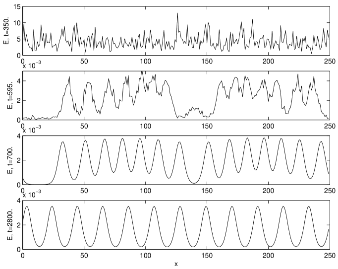
Figure 1: Energy contour for a $1D$ system at different stages of the evolution. The top plot shows the initial thermal configuration followed by a snapshot characteristic of early times after the quench to $T=0$. At later times the kink network evolves to form a stable wall lattice as shown in the bottom plot.

Our goal here is to check whether a stable kink lattice forms in one spatial dimension as an initial “hot” configuration is quenched to $T=0$. Applying the procedure detailed in the previous section to the system, we confirm that this is in fact the case. In Fig. 1 we show a series of snapshots of the energy profile of the fields for different times in a typical simulation run. The first configuration corresponds to the end of the thermalization phase, with large amplitude fluctuations and very uncorrelated fields. At this point we turn the stochastic term off and let the system evolve for a considerably long time. In this case we keep the dissipation high since we are not interested in the details of the dynamics of the system but rather in observing a stable lattice as the final outcome. As the energy is then dissipated, a recognisable pattern of “proto-kinks” starts to form, as can be seen in the second snapshot. The next energy profile shows that the field has relaxed to a fully formed network of kinks. During further evolution, neighbouring attractive kink-antikink pairs annihilate, leading to a stable lattice of equidistant domain walls. This final state is shown in the fourth plot, a succession of mutually repelling kinks and antikinks. The energy of these defects corresponds to the value predicted analytically, and direct inspection of the values of the four fields $f_{i}$ confirms that, as expected, we are in presence of a genuine domain wall lattice.

III.3 Simulation in ($2+1$)D

After having established that in one spatial dimension kink lattices can form as a consequence of a phase transition, we will now look at the evolution of the same model in the (2+1)D case. Here we expect the late time dynamics of the system to be dominated by networks of one-dimensional domain walls. As a consequence of the symmetry content of the model, these networks will be considerably more complex than the ones based on ordinary $Z_{2}$ walls. In particular, we can expect walls to intersect and kink-antikink repulsion to play a role in the evolution.

Our first task is to find a method to identify the walls starting from the field values in the simulation lattice. To this end it is convenient to convert the fields $f_{i}(x)$ back into the original $SU(5)\times Z_{2}$ matrix form, $\Phi(x)$. For any type of kink in the model, there is at least one element $\Phi_{jj}$ of the diagonal of the field matrix that changes sign as one crosses the defect core PogVac00 ; Vac01 ; PogVac01 . In the particular case of the lowest energy kinks, those described by the charge matrices $Q^{(i)}$, it is easy to see that only one of the $\Phi_{jj}$’s changes sign. For these cases, ${\rm Tr}[\Phi^{3}]$ also vanishes at the defect’s core. Since this does not happen for any of the other kink types, we have a way of distinguishing between the least energetic kinks and general unstable ones. We thus measure at each time step the total number of zero crossings between all adjacent lattice points, of both the $\Phi_{jj}$’s and of ${\rm Tr}[\Phi^{3}]$. For most of the evolution the network consists predominantly of stable kinks and the two quantities coincide, defining the total wall length in the system.

The simulations follow the same pattern as before, starting with a thermalization stage after which the stochastic term in the equation of motion is set to zero. In this case, however we are interested in studying the long time scaling behaviour of the network. Since we are mostly concerned with the relativistic limit of the theory the dissipation term must be set to zero during the scaling period. Nevertheless, since the initial thermal configuration is very energetic, we keep the dissipation high for some time after the quench, before setting $D=0$ for the scaling regime. In this way, some of the excess energy is dissipated away, allowing the fields to relax into a well formed network configuration that then can start scaling.

In all simulations, the model parameters and space and time discretization steps used were the same as in the one dimensional runs. The fields were evolved in a $N=2500^{2}$ point grid.

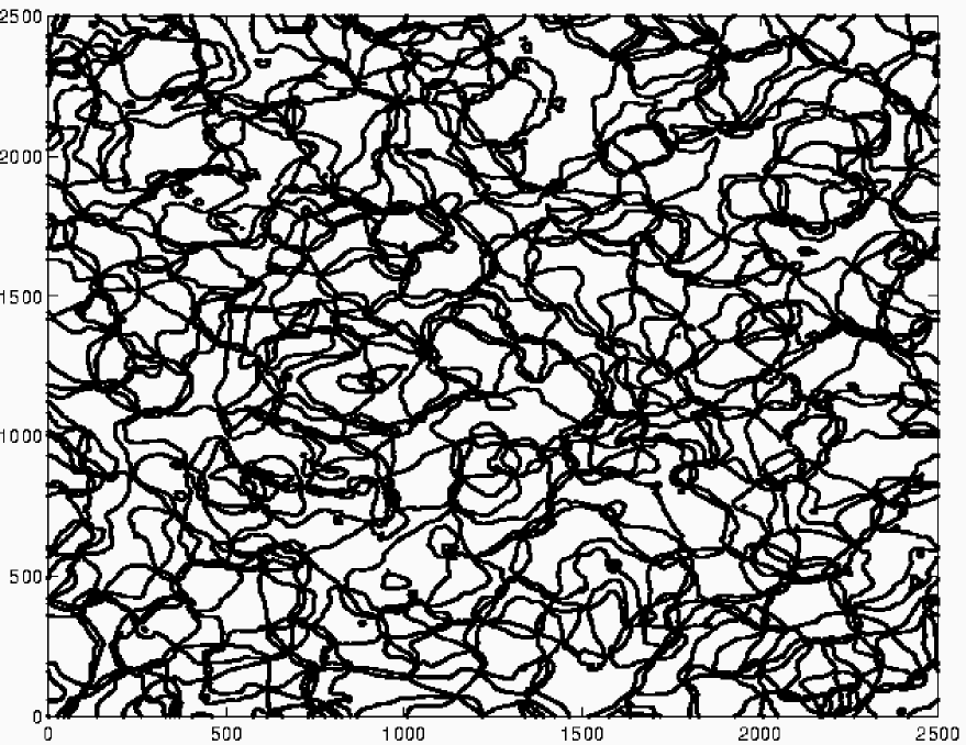
Figure 2: High density wall network for an early evolution time, $t=400$.

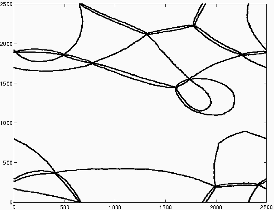
Figure 3: Late time network configuration $t=3200$.

In Fig. 2 we can see a snapshot of the wall network for an early time in the scaling period, $t=400$. The network is very dense with a very high number of intersections. The walls were identified using the method discussed above. At this time all the kinks in the network are stable and the number of zero crossings for the $\Phi_{jj}$’s and for ${\rm Tr}[\Phi^{3}]$ coincide. By direct observation of the field configurations, we confirmed that higher energy kinks do exist for earlier times which quickly decay into stable ones. A secondary consequence of such decay processes is that stable kinks forming in pairs from a single unstable kink tend to remain spatially correlated near junctions. Since the repulsive force between kinks is exponentially small, this pairing is relatively stable and can be observed for considerably late times (see Fig. 3).

For later times most walls annihilate, loops form and decay into radiation and the overall density decreases. Walls tend to get straighter as this is energetically more favourable, though the time-scale relevant for this process is clearly larger than the decay time of the network. In Fig. 3 we show the network for a later time, $t=3200$. The reduction in density is remarkable, with only a small number of intersecting walls remaining. The way these intersect to form nodes is quite interesting and we can see in particular that around each node there are always six incoming walls. This is related to the fact that the minimal periodic wall lattice is composed of six walls, as discussed in Section II. It is clear that for such a configuration to be stable for very long times, the walls around the node must repel each other. Hence the sequence of their charges must correspond to a stable wall lattice pattern. For earlier times we observe nodes with other numbers of incoming walls, though, as expected, never less than six. High index nodes are rarer because they are both less likely to form and more likely to cancel with other nodes to form a minimal six wall configuration. Eventually all nodes annihilate with anti-nodes with reversed “vacuum orientation”, and for very long times all walls disappear. In all the simulations performed in a square lattice, the final state always had zero wall content and a two dimensional wall lattice never formed. Nevertheless, we observed that by taking one of the linear dimensions of the simulation domain $L_{y}$ to be smaller than the other $L_{x}$, a regular lattice of straight parallel walls can be obtained as the outcome of the evolution. Though more careful simulations need to be performed, our preliminary results suggest that as the smaller grid dimension increases, the final density of walls in the lattice becomes smaller. When $L_{y}/L_{x}$, the ratio of the two dimensions becomes larger than roughly $1/3$, no lattice is formed. This result can be better understood by imagining the limit when one of the torus dimensions (say $L_{y}$) goes to zero and the 1D case is recovered. In this situation, the final state of the evolution should be a series of parallel walls crossing the torus in the $y$-direction. As $L_{y}$ increases, we can expected that some of these walls will be able to “explore” the torus in both the $x$ and $y$-directions. Some of these will not cross the torus, getting linked to other walls and forming a complex network. As the network evolves, wall nodes will annihilate, some of these annihilations further decreasing the number of walls that cross the box in the $y$-direction. As a result, the final state of the system will still be a set of straight repelling parallel walls in the $y$-direction, but with a lower density. It is easy to imagine that as $L_{y}$ increases and approaches $L_{x}$, the final density will decrease, up to the point where no lattice will form at all. The fact that the final state of the transition depends on the geometry of the system is unexpected and may have implications in cosmological settings in models with extra dimensions. Still, a better understanding of this phenomenon and the mechanisms behind it is needed before further conclusions can be drawn.

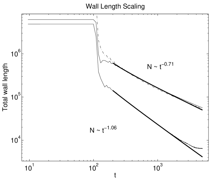
Figure 4: Wall length versus time for both the $S_{5}\times Z_{2}$ theory (top curve) and the single field $Z_{2}$ case (bottom curve). The dashed curve corresponds to the total $S_{5}\times Z_{2}$ wall length measured by counting zeros of the diagonal elements of $\Phi(x)$. Except for very early times this coincides with the number of zeros of ${\rm Tr}[\Phi^{3}]$ (solid curve). The results shown are averages of $25$ independent realizations. In all cases, for $t<100$ the system is evolved with both non-zero dissipation and thermal noise. At $t=100$ we quench the system to zero temperature but the dissipation term is kept until $t=125$ to eliminate excess energy. For $t>125$ we set $D=0$. The power-law fits (bold lines) to both curves were taken between $t=200$ and $t=1350$. For later times (larger than half the simulation box length) finite size effects become significant.

Another indication that the dynamics of this system differs fundamentaly from regular defect networks can be obtained by studying its scaling properties. In Fig. 4 we show a $log-log$ plot of the total wall length versus time. For comparison we also include a plot of the scaling of a regular $Z_{2}$ domain wall network. This was obtained by evolving a scalar $\lambda\phi^{4}$ theory in parallel with the $S_{5}\times Z_{2}$ system. In both cases after the initial thermalization and dissipation periods, the domain wall network enters a scaling regime where the time evolution of the total wall length is well described by a power-law $N\sim t^{-\alpha}$. For the $Z_{2}$ theory we find $\alpha=1.06(0.06)$ which is in reasonable agreement with both previous theoretical and numerical predictions of $\alpha=1.$ (see GarHin02 and references therein). This is to be compared with the result for the $S_{5}\times Z_{2}$ walls. In this case we find $\alpha=0.71(0.02)$, a considerably lower result. Clearly, the dynamics of the $S_{5}\times Z_{2}$ network is fundamentally different from the $Z_{2}$ case. This is not surprising, taking into account that the process of node/anti-node annihilation must play an important role in the dynamics of the system. That the overall effect is a slowdown in the scaling, could also be expected on the basis that the six-wall junctions feel a force that is predominantly isotropic. This suggests that systems allowing for stable nodes with higher number of crossing walls and hence more isotropic, would be likely to display even lower scaling powers. In the limit of infinite number of incoming walls per node the system would eventually become static.

IV Conclusions

We have numerically studied phase transitions in a model with $S_{5}\times Z_{2}$ symmetry breaking down to $S_{3}\times S_{2}$ in one and two spatial dimensions. In one dimension, as expected, we find that a stable domain wall lattice forms. In two dimension, we observed the formation of a complicated network of domain walls and domain wall junctions. At every junction six domain walls are present. With time, the junctions move and annihilate, and the network coarsens. This feature of the network dynamics leads to a slowdown of the scaling regime. We found that the total length of domain wall in the network scales as $t^{-0.71}$, in contrast to the $t^{-1.0}$ fall off expected for $Z_{2}$ domain walls in a $\lambda\phi^{4}$ model.

We have not studied the phase transition in three dimensions since the problem then becomes computationally very intensive. Even then our results can be extrapolated to three dimensions, allowing us to anticipate certain behavior. In three dimensions we expect the wall junctions to be one dimensional – somewhat like strings. The network of walls will coarsen as the strings come together and annihilate. This is very reminiscent of a system of cosmic strings in which each string then gets connected to six domain walls and the evolution of the networks should be similar KubIsiNam90 ; Kub92 ; RydPreSpe90 ; VilShe94 . The new feature in the present case is the repulsion between walls and antiwalls and this could lead to lattice formation at very late times.

Perhaps the most important application of our study is to the $SU(5)\times Z_{2}$ case as this is a realistic particle physics model. As we have noted in Sec. II, the domain walls in the $SU(5)$ model are identical to those in the $S_{5}$ model. The difference is only in their stability properties. Hence we might expect some of the features of the domain wall networks in the $S_{5}$ case to carry over to the $SU(5)$ case. Exactly how much similarity will survive is hard to predict and may depend on model parameters. This remains an important problem to explore.

- (1) L. Pogosian and T. Vachaspati, Phys. Rev. D64, 105023 (2001).
- (2) L. Pogosian and T. Vachaspati, Phys. Rev. D62, 123506 (2000).
- (3) T. Vachaspati, Phys. Rev. D63, 105010 (2001).
- (4) A. Davidson, B. F. Toner, R. R. Volkas and K. C. Wali, Phys. Rev. D65, 125013 (2002).
- (5) L. Pogosian, Phys. Rev. D65, 065023 (2002).
- (6) T. Vachaspati, hep-th/0303137.
- (7) D. Tong, Phys. Rev. D66, 025013 (2002).
- (8) B.S. Ryden, W.H. Press and D.N. Spergel, Ap. J. 357, 293 (1990).
- (9) H. Kubotani, H. Ishihara and Y. Nambu, Prepared for (IUPAP) International Conference on Primordial Nucleosynthesis and Evolution of the Early Universe, Tokyo, Japan, 4-8 Sep 1990
- (10) H. Kubotani, Prog. Theor. Phys. 87, 387 (1992).
- (11) L. Pogosian and T. Vachaspati, Phys. Rev. D67, 065012 (2003).
- (12) T. Garagounis and M. Hindmarsh, hep-ph/0212359
- (13) A. Vilenkin and E.P.S. Shellard, “Cosmic Strings and Other Topological Defects”, Cambridge University Press (1994).