CERN-TH 2003-155
DESY 03–084
hep-ph/0307346
July 2003

Hadronic Higgs Production and Decay in Supersymmetry at Next-to-Leading Order

Abstract

Supersymmetric QCD corrections to the gluonic production and decay rate of a CP-even Higgs boson are evaluated at next-to-leading order. To this aim, we derive an effective Lagrangian for the gluon-Higgs coupling. We show that a consistent calculation requires the inclusion of gluino effects, in contrast to what has been done previously. The supersymmetric corrections to the gluon-Higgs coupling lead to a modification of the next-to-leading order K-factor for the Higgs production rate at the LHC by less than 5%.

1 Introduction

It is among the main goals of the CERN Large Hadron Collider (LHC) to observe the Higgs boson and study its properties. The most important production mechanisms for a Standard Model (SM) Higgs boson have been studied in great detail and are known with fairly high theoretical precision (for a review, see Refs. [3, 4, 5]). The dominant mode is gluon fusion, where, at leading order in perturbation theory, the gluons couple to the Higgs boson preferably via a top quark loop. A light Higgs boson, $M_{H}\leq 130$ GeV, would be observed through its subsequent decay into photon pairs. For larger values of the Higgs boson mass, $H\to ZZ^{(\ast)}$ and $H\to WW^{(\ast)}$ allow for a clear identification of the Higgs signal.

The next-to-leading order (NLO) corrections to the gluon fusion process in the Standard Model are known exactly [6, 7, 4]. They were shown to be approximated extremely well by an earlier calculation which was based on the heavy-top limit [8, 9]. This is true for a large range of the Higgs mass, including even $M_{H}>2\,M_{t}{}$, provided that the mass dependence at leading order in $\alpha_{s}$ is kept exactly. Recently, the next-to-next-to-leading order (NNLO) corrections in the heavy-top limit became available [10, 11] (see also Ref. [12]). They lead to a significant stabilization of the theoretical prediction, with a remaining scale uncertainty of around 15%. The SM Higgs production rate at the LHC is thus under good theoretical control.

In the Minimal Supersymmetric Standard Model (MSSM), several aspects have to be taken into account when considering the production of a neutral scalar Higgs boson: For example, for large $\tan\beta$, the bottom quark can contribute significantly to the gluon-Higgs coupling. This effect has been studied at NLO in Refs. [6, 13, 7, 4]. A large value of $\tan\beta$ also brings in the associated production of a Higgs boson with bottom quarks as one of the main production mechanisms [14, 15, 16].

The main subject of the current paper are the contributions of MSSM particles to the gluon-Higgs coupling. At sufficiently small values of $\tan\beta$, the dominant effects are due to top-squarks and gluinos. The NLO squark contributions have been addressed in Ref. [17]. However, as we will show, these results do not correspond to a consistent supersymmetric framework. In fact, it turns out that the squark contributions can not be separated from the gluino effects. This will significantly affect the final result, most evidently in the appearance of non-decoupling logarithmic contributions from the gluino mass.

Motivated by its success in the SM case, we construct an effective Lagrangian at NLO for the gluon-Higgs interaction in the MSSM. This corresponds to integrating out the top quark and all supersymmetric particles. Within the framework of this effective Lagrangian, all calculations can be performed in standard five-flavor QCD. They can thus be taken over from the SM case.

In this paper, we restrict ourselves to the case without squark mixing, and focus on a principle study of the method. A more general analysis will be presented in a forthcoming paper.

2 The effective Lagrangian in supersymmetric QCD

2.1 General definition

It has been shown that the radiative corrections to the production rate of a SM Higgs boson are well described by an effective theory, where formally the top quark is assumed much heavier than the Higgs boson. In practice, it turns out that this approximation works very well even way beyond the formal limit $M_{t}{}>M_{H}$. We therefore assume that a similar behavior will be observed in the MSSM, and construct an effective Lagrangian where the top quark, the squarks, and the gluino are integrated out. The Higgs boson itself enters only as external particle and thus the Lagrangian describing the effective $\phi gg$ coupling at leading order in $M_{\phi}$ has the form

$${\cal L}_{Y,\rm eff} = -\frac{\phi^{0}}{v^{0}}C_{1}^{0}{\cal O}_{1}^{0}\,,\qquad{\cal O}_{1}^{0}=\frac{1}{4}G_{\mu\nu}^{0}G^{0,\mu\nu}\,,$$ (1)

where $C_{1}^{0}$ is the coefficient function containing the remnant contribution of the heavy particles and ${\cal O}_{1}^{0}$ is the effective operator. $\phi$ denotes either of the two CP-even Higgs bosons of the MSSM. $G_{\mu\nu}^{0}$ is the gluonic field strength tensor of standard, five-flavor QCD. The superscript “0” indicates bare quantities as opposed to renormalized ones. Note that the renormalization of $\phi^{0}/v^{0}$ is of higher order in the electromagnetic coupling constant.

The renormalization of $C_{1}^{0}$ and ${\cal O}_{1}^{0}$ is discussed in Ref. [18, 19] and is given by

$$\begin{split}C_{1}&=Z_{11}^{-1}\,C_{1}^{0}\,,\qquad{\cal O}_{1}=Z_{11}\,{\cal O}_{1}^{0}\,,\qquad Z_{11}=\left(1-\frac{\pi}{\alpha_{s}}\frac{\beta}{\epsilon}\right)^{-1}\,,\end{split}$$ (2)

where $\beta(\alpha_{s})$ is the $\beta$-function of standard $(n_{l}=5)$-flavor QCD:

$$\begin{split}\mu^{2}\frac{{\rm d}}{{\rm d}\mu^{2}}\frac{\alpha_{s}}{\pi}=\beta(\alpha_{s})\,,\end{split}$$ (3)

with $\beta(\alpha_{s})=-(\alpha_{s}/\pi)^{2}\beta_{0}+\ldots$ and $\beta_{0}=11/4-n_{l}/6$. Note that here and in what follows, $\alpha_{s}$ denotes the strong coupling constant in standard five-flavor QCD; it is a function of the renormalization scale $\mu$:

$$\begin{split}\alpha_{s}\equiv\alpha_{s}^{(5)}(\mu)\,.\end{split}$$ (4)

According to Eq. (1), the calculation of the gluonic Higgs production cross section or the decay rate splits into two parts: On the one hand, the coefficient function $C_{1}$ has to be determined to the desired order. This part is independent of the process considered; the result will be useful for any process to which the effective Lagrangian approach is applicable. The second part of the calculation is to evaluate the production or decay rate on the basis of the operator ${\cal O}_{1}$ within five-flavour QCD.

In the SM, the coefficient function $C_{1}$ is known to order $\alpha_{s}^{4}$. The $\alpha_{s}^{2}$-terms have been computed in Refs. [20, 9], while the contributions of order $\alpha_{s}^{3}$ were obtained in Refs. [21, 19] (see also Ref. [22]), and the terms of order $\alpha_{s}^{4}$ in Ref. [19]. For later reference, let us quote the NLO result at this point:

$$\begin{split}C_{1}^{\rm SM}(\alpha_{s})&=-\frac{\alpha_{s}}{3\pi}\left(1+\frac{11}{4}\frac{\alpha_{s}}{\pi}\right)+{\cal O}(\alpha_{s}^{3})\,.\end{split}$$ (5)

Within the SM framework, there exists an all-order low-energy theorem [19] which expresses $C_{1}^{\rm SM}$ in terms of $\beta(\alpha_{s})$ and $\gamma_{m}(\alpha_{s})$, the anomalous dimensions of $\alpha_{s}$ and $M_{t}{}$, respectively. The result of Ref. [17] for the squark-contribution to the effective theory at order $\alpha_{s}^{2}$ was derived by replacing the $\beta$-function with its pure squark contribution, and $\gamma_{m}$ with the anomalous dimension of the squark mass. The obtained expression was multiplied by a factor $\propto(M_{t}/\tilde{M}_{t})^{2}$, unaffected by renormalization.

Our explicit calculation shows that for the correct effective Higgs-gluon coupling, the top squark contribution can not be considered on its own. In fact, as soon as the proper renormalization of the Higgs-squark coupling is taken into account, the pure squark contribution receives ultra-violet divergences which are canceled by a contribution coming from top quarks and gluinos, like the ones in Fig. 2 $(c)$, $(d)$. As a consequence of this important conceptual difference, also the numerical results for hadronic Higgs production have to be re-analyzed.

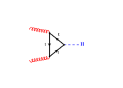
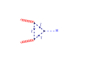
$(a)$	$(b)$

Figure 1: One-loop Feynman diagrams contributing to gluon fusion in the MSSM.

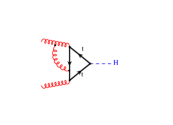
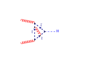
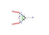
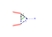
$(a)$	$(b)$	$(c)$	$(d)$

Figure 2: Sample two-loop Feynman diagrams contributing to gluon fusion in the MSSM. Apart from the pure QCD corrections to the top quark $(a)$ and top squark $(b)$ triangle, there are also corrections involving the gluino $(c)$, $(d)$.

In this paper, we follow the diagrammatic approach of Refs. [21, 19] in order to evaluate the effective Higgs-gluon interaction in the MSSM, including terms of order $\alpha_{s}^{2}$. As explained above, this involves three types of two-loop Feynman diagrams: Gluonic corrections to top quark loops, e.g. Fig. 2 $(a)$; gluonic corrections to top squark loops, e.g. Fig. 2 $(b)$; gluino-contributions, e.g. Fig. 2 $(c)$, $(d)$. The resulting effective Lagrangian can then be used to evaluate the Higgs production rate at a hadron collider to NLO.

2.2 Calculational details

It is well known that Dimensional Regularization (DREG) [23] breaks supersymmetry. This can be cured by adding finite counterterms that restore the supersymmetric Ward identities. Alternatively, one can choose a regularization procedure which preserves supersymmetry. A viable method which is very similar to DREG is Dimensional Reduction (DRED) [24] (see also [25]). The essential difference to DREG is that the tensor algebra is performed in four instead of $D=4-2\epsilon$ dimensions, whereas the loop integrals are still $D$ dimensional. We checked that the final result is the same, both in DRED and in DREG, provided the aforementioned finite counterterms are taken into account.

The generation and evaluation of the Feynman diagrams proceeds fully automatically through the chain

QGRAF	$\to$	Q2E	$\to$	EXP	$\to$	MATAD/MINCER
[26]		[27]		[28]		[29]/[30]
generation		analyzation		asymptotic expansion		calculation

Q2E translates the output of QGRAF into a format that is suitable for further manipulation. EXP applies asymptotic expansions on a diagrammatical level, according to a user-defined hierarchy of mass (possibly also momentum) scales, and produces output that can be given to the integration packages MINCER and MATAD immediately. The latter use the Integration-by-Parts algorithm [31] in order to evaluate the single-scale integrals analytically.

2.3 The effective Lagrangian at next-to-leading order

Various methods for the evaluation of $C_{1}$ are described in Refs. [19, 32]. We follow the most direct one, which means to apply the projector

$$\begin{split}P_{\mu\nu}^{ab}(p_{1},p_{2})=\delta^{ab}\,\frac{p_{1}\cdot p_{2}\,g_{\mu\nu}-p_{1\nu}p_{2\mu}-p_{1\mu}p_{2\nu}}{8\,(D-2)(p_{1}\cdot p_{2})^{2}}\end{split}$$ (6)

to the $gg\phi$ vertex diagrams (sample diagrams are shown in Figs. 1 and 2), and evaluating them at $p_{1}=p_{2}=0$. Here, $\mu$, $\nu$ and $a$, $b$ are the Lorentz and color indices of the external gluons, and $p_{1}$, $p_{2}$ are their momenta. This will result in the product $\zeta_{3}^{0}\,C_{1}^{0}$, where $\zeta_{3}^{0}$ is the bare decoupling constant of the gluon field obtained from the one-loop gluon propagator involving top quarks, top squarks, and gluinos:

$$\begin{split}\zeta_{3}^{0}&=1+\frac{\alpha_{s}}{\pi}\bigg{(}\frac{3}{4\epsilon}+L(\epsilon)\bigg{)}+{\cal O}(\alpha_{s}^{2})\,,\qquad\mbox{with}\\ L(\epsilon)&=\frac{1}{24}\left(12\,L_{g}+L_{L}+L_{R}+4\,L_{t}\right)+\frac{\epsilon}{12}\left(3\,L_{g}^{2}+\frac{1}{4}\left(L_{L}^{2}+L_{R}^{2}\right)+L_{t}^{2}+\frac{9}{2}\,\zeta_{2}\right)\,,\end{split}$$ (7)

$$\begin{split}L_{t}&=\ln\frac{\mu^{2}}{M_{t}^{2}}\,,\qquad L_{L}=\ln\frac{\mu^{2}}{\tilde{M}_{L}^{2}}\,,\qquad L_{R}=\ln\frac{\mu^{2}}{\tilde{M}_{R}^{2}}\,,\qquad L_{g}=\ln\frac{\mu^{2}}{\tilde{M}_{g}^{2}}\,,\end{split}$$ (8)

and $\zeta_{2}\equiv\pi^{2}/6$. $\tilde{M}_{L/R}$ is the mass for the supersymmetric partner of the left/right-handed top quark, $\tilde{M}_{g}$ is the gluino mass, and $M_{t}$ the top quark mass. One-loop renormalization of the strong coupling constant and the masses (see, e.g., Ref. [33]) leads to $C_{1}(\tilde{\alpha}_{s})$, where $\tilde{\alpha}_{s}$ is the renormalized coupling constant in the full theory. It is related to $\alpha_{s}$, the coupling in standard five-flavor QCD (see Eq. (4)), by

$$\begin{split}\alpha_{s}=(\zeta_{g})^{2}\,\tilde{\alpha}_{s}\,,\qquad\mbox{where}\qquad\zeta_{g}^{2}=1-\frac{\alpha_{s}}{\pi}L(\epsilon)+{\cal O}(\alpha_{s}^{2})\,.\end{split}$$ (9)

$L(\epsilon)$ is defined in Eq. (7).

For brevity, we will focus on the following two cases in this letter:

$$\begin{split}(A)\qquad&\tilde{M}_{g}{}\gg\tilde{M}_{L}=\tilde{M}_{R}\equiv\tilde{M}_{t}{}\sim M_{t}{}\,,\\ (B)\qquad&\tilde{M}_{R}\gg\tilde{M}_{g}{}\gg\tilde{M}_{L}\sim M_{t}{}\,,\end{split}$$ (10)

These cases are motivated by the fact that the supersymmetric (SUSY) contributions to the gluon-Higgs coupling are proportional to $M_{t}{}^{2}/\tilde{M}_{t}{}^{2}$. Sizable effects are thus only expected if at least one of the top squarks has a mass of the order of the top quark mass. Bottom squark contributions are suppressed by $(M_{b}/\tilde{M}_{b})^{2}\cdot\tan\beta$ and can savely be neglected for not-too-large values of $\tan\beta$, as we assume them in this paper. Furthermore, as already mentioned in the Introduction, we do not consider the mixing of the top squarks.

The one-loop calculation of $C_{1}$ involves only diagrams with a single mass scale: $\tilde{M}_{t}{}$ or $M_{t}{}$. At two-loop order, up to three different masses can appear in the loop diagrams (see, e.g., Fig. 2 $(c)$, $(d)$), which makes the calculation quite tedious. However, adopting the hierarchies of the cases $(A)$ and $(B)$ introduced above, one can apply asymptotic expansions [34] (see also Ref. [35] for pedagogic examples) in order to reduce the multi-scale to single-scale Feynman diagrams. This leads to significantly simpler integrals and final results of a handy structure (powers and logarithms of the masses).

For later convenience, we parametrize the SUSY contributions to the coefficient function in the following way:

$$\begin{split}C_{1}&=g_{t}^{\phi}\,C_{1}^{\rm SM}\,c_{0}(x_{tL},x_{tR})\left[1+\frac{\alpha_{s}}{\pi}\,c^{\rm SUSY}\right]\,,\qquad\mbox{where}\end{split}$$ (11)

$$\begin{split}c_{0}(x_{tL},x_{tR})&=1+\frac{1}{4}\left(x_{tL}+x_{tR}\right)\,,\qquad x_{tL}=\frac{M_{t}^{2}}{\tilde{M}_{L}^{2}}\,,\qquad x_{tR}=\frac{M_{t}^{2}}{\tilde{M}_{R}^{2}}\,.\end{split}$$ (12)

$g_{t}^{\phi}$ represents the coupling of the Higgs boson to top quarks which is specified below. We evaluate case $(A)$ of Eq. (10) by first considering the following subcase:

$$\begin{split}(A^{\prime})\qquad&\tilde{M}_{g}{}\gg\tilde{M}_{L}=\tilde{M}_{R}\equiv\tilde{M}_{t}{}\gg M_{t}{}\,.\end{split}$$ (13)

Expressing the top quark and squark mass in the on-shell scheme, one gets:

$$\begin{split}c^{\rm SUSY}[A^{\prime}]&=\frac{x_{ts}}{c_{0}(x_{ts},x_{ts})}\bigg{[}a^{(0)}+x_{tg}\,a^{(1)}+x_{tg}^{2}\,a^{(2)}+{\cal O}(x_{tg}^{3})\bigg{]}+{\cal O}(\alpha_{s})\,,\end{split}$$ (14)

$$\begin{split}a^{(0)}&=\frac{11}{8}+\frac{1}{3}L_{gs}+L_{tg}\,,\qquad a^{(1)}=\frac{1}{18}-\frac{3}{4}L_{gs}+\frac{11}{12}L_{tg}+x_{ts}\,\left(\frac{14}{9}+\frac{4}{3}L_{tg}\right)\,,\\ a^{(2)}&=-\frac{157}{36}+\zeta_{2}-\frac{3}{4}L_{gs}-\frac{7}{12}L_{tg}-\frac{1}{2}L_{gs}L_{tg}\\ &\quad+x_{ts}\left(-\frac{37}{9}+\zeta_{2}-\frac{13}{12}L_{gs}-\frac{7}{12}L_{tg}-\frac{1}{2}L_{gs}L_{tg}\right)+x_{ts}^{2}\,\left(\frac{25}{12}+3\,L_{tg}\right)\,,\end{split}$$ (15)

with

$$\begin{split}x_{ts}&=\frac{M_{t}^{2}}{\tilde{M}_{t}^{2}}\,,\qquad x_{tg}=\frac{\tilde{M}_{t}^{2}}{\tilde{M}_{g}^{2}}\,,\qquad L_{tg}=\ln\frac{M_{t}^{2}}{\tilde{M}_{g}^{2}}\,,\qquad L_{gs}=\ln\frac{\tilde{M}_{g}^{2}}{\tilde{M}_{t}^{2}}\,.\end{split}$$ (16)

In the numerical analysis of Section 3, the coefficients $a^{(i)}$ are included up to $i=6$. Note that the explicit $\mu$ dependence drops out which has to be the case as the anomalous dimension of $C_{1}$ has to cancel the $\mu$ dependence of $\alpha_{s}$ in the one-loop term (cf. Eq. (2)). This is a strong check for our calculation.

An observation concerning Eq. (15) is that the two-loop contribution of order $M_{t}{}^{2}/M_{\tilde{t}}^{2}$ depends logarithmically on $\tilde{M}_{g}{}$ which is a consequence of the simultaneous decoupling of all heavy particles. However, in the limit that all SUSY particles are heavy, as expected, the SM result is recovered. Let us add that the bare two-loop result even has contributions $\propto\tilde{M}_{g}{}^{2}\cdot M_{t}{}^{2}/\tilde{M}_{t}{}^{2}$, but those are canceled by the on-shell counter term of the squark mass.

Another remarkable observation concerning Eq. (15) is that higher order terms in $M_{t}{}^{2}/\tilde{M}_{t}^{2}$ identically vanish, i.e., the coefficients $a^{(i)}$, $i=0,1,2,\ldots$ are exact. This means that Eq. (15) is valid for arbitrary values of $M_{t}{}$ and $\tilde{M}_{t}{}$, provided that $\tilde{M}_{g}{}$ is sufficiently large. In particular, it covers case $(A)$ of Eq. (10):

$$\begin{split}c^{\rm SUSY}[A]\equiv c^{\rm SUSY}[A^{\prime}]\,.\end{split}$$ (17)

This equality has been checked up to order $1/\tilde{M}_{g}^{16}$, and it is suggestive that it holds to all orders in the inverse gluino mass.

In order to quantify the condition $\tilde{M}_{g}{}\gg(M_{t}{},\tilde{M}_{t}{})$, we show in Fig. 3 the expansion of Eq. (15), including successively higher orders in $x_{sg}=\tilde{M}_{t}^{2}/\tilde{M}_{g}^{2}$, for fixed values of $x_{ts}$. One clearly observes that the expansion breaks down dramatically beyond a certain value of $x_{sg}$. However, we conclude that for $\tilde{M}_{g}\gtrsim 2.5\,\tilde{M}_{t}$ and $\tilde{M}_{t}\geq M_{t}$, the expansion should be accurate to better than $1\%$. Note also that, as mentined above, the expression diverges logarithmically like $\ln(x_{sg})$ as $x_{sg}\to 0$.

As an interesting special case, let us consider the limit $\tilde{M}_{L}=\tilde{M}_{R}=M_{t}{}$ which leads to the compact formula

$$\begin{split}C_{1}[\tilde{M}_{L}=\tilde{M}_{R}=M_{t}]&=-g_{t}^{\phi}\frac{\alpha_{s}}{2\pi}\left[1+\frac{\alpha_{s}}{\pi}\left(\frac{11}{3}+\frac{4}{9}L_{tg}\right)\right]+{\cal O}(\frac{M_{t}^{2}}{\tilde{M}_{g}^{2}},\alpha_{s}^{3})\end{split}$$ (18)

It is worth noting that the coefficient $a^{(0)}$ in Eq. (15) is positive only for $\tilde{M}_{g}<e^{33/32}M_{t}\approx 2.8M_{t}$.

Considering case $(B)$ of Eq. (10), we proceed in complete analogy to case $(A)$, i.e., we first evaluate the subcase

$$\begin{split}(B^{\prime})\qquad\tilde{M}_{R}\gg\tilde{M}_{g}{}\gg\tilde{M}_{L}\gg M_{t}{}\,.\end{split}$$ (19)

Keeping only the leading term in $1/\tilde{M}_{R}$ at NLO, we find

$$\begin{split}c^{\rm SUSY}[B^{\prime}]&=\frac{x_{tL}}{c_{0}(x_{tL},x_{tR})}\,\bigg{[}b^{(0)}+x_{Lg}\,b^{(1)}+x_{Lg}^{2}\,b^{(2)}+{\cal O}(x_{tR},x_{Lg}^{3})\bigg{]}+{\cal O}(\alpha_{s})\,,\end{split}$$ (20)

$$\begin{split}b^{(0)}&=\frac{29}{48}+\frac{L_{gR}}{12}+\frac{L_{gL}}{6}+\frac{L_{tg}}{2}\,,\\ b^{(1)}&=-\frac{1}{18}-\frac{5}{24}L_{gL}+\frac{11}{24}L_{tg}+x_{tL}(\frac{13}{18}+\frac{2}{3}L_{tg})\,,\\ b^{(2)}&=-\frac{163}{72}+\frac{1}{2}\zeta_{2}-\frac{1}{8}L_{gL}-\frac{7}{24}L_{tg}-\frac{1}{4}L_{gL}L_{tg}\\ &\quad+x_{tL}\left(-\frac{85}{36}+\frac{1}{2}\zeta_{2}-\frac{3}{8}L_{gL}-\frac{7}{24}L_{tg}-\frac{1}{4}L_{gL}L_{tg}\right)+x_{tL}^{2}\left(\frac{49}{48}+\frac{3}{2}L_{tg}\right)\,,\end{split}$$ (21)

where

$$\begin{split}x_{tL}&=\frac{M_{t}^{2}}{\tilde{M}_{L}^{2}}\,,\qquad x_{tR}=\frac{M_{t}^{2}}{\tilde{M}_{R}^{2}}\,,\qquad x_{Lg}=\frac{\tilde{M}_{L}^{2}}{\tilde{M}_{g}^{2}}\,,\\ L_{tg}&=\ln\frac{M_{t}^{2}}{\tilde{M}_{g}^{2}}\,,\qquad L_{gL}=\ln\frac{\tilde{M}_{g}^{2}}{\tilde{M}_{L}^{2}}\,,\qquad L_{gR}=\ln\frac{\tilde{M}_{g}^{2}}{\tilde{M}_{R}^{2}}\,.\end{split}$$ (22)

We again evaluated the coefficients up to order $x_{tR}^{6}$ and $x_{Lg}^{6}$ and use them in the numerical analyses below. Note that this result still has a logarithmic dependence on $\tilde{M}_{R}$; this comes in addition to the logarithmic dependence on $\tilde{M}_{g}$ as $\tilde{M}_{g}\to\infty$, as it was already observed in case $(A)$.

Also in analogy to case $(A)$, the coefficients $b^{(i)}$, $i=0,1,2,\ldots$ are exact, meaning that Eq. (21) also covers case $(B)$:

$$\begin{split}c^{\rm SUSY}[B]=c^{\rm SUSY}[B^{\prime}]\,.\end{split}$$ (23)

For sufficiently large values of $\tilde{M}_{R}$, an analogous study as in case $(A)$ to quantify the condition $\tilde{M}_{g}\gg(\tilde{M}_{L},M_{t})$ leads to very similar conclusions, so that we refrain from presenting it here.

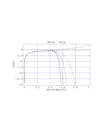
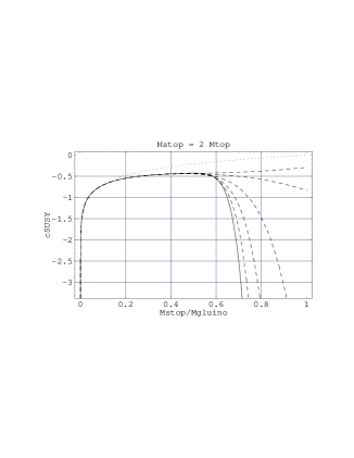
$(a)$	$(b)$

Figure 3: $c^{\rm SUSY}$ for Case $(A)$ of Eq. (10) with $(a)$ $\tilde{M}_{t}{}=M_{t}{}$ and $(b)$ $\tilde{M}_{t}{}=2M_{t}{}$, as a function of the ratio $\tilde{M}_{t}{}/\tilde{M}_{g}{}$. The individual lines correspond to different orders of the expansion in the square of this ratio. The dotted line includes only the leading term, whereas the solid line incorporates corrections up to order $(\tilde{M}_{t}/\tilde{M}_{g})^{12}$.

3 Higgs Decay Rate and Production Cross Section

3.1 Decay rate

From Eq. (1) one can derive a general expression for the inclusive $\phi\to gg$ decay width,

$$\Gamma(\phi\to gg)=\Gamma_{0}\left(1+\delta\right)\,,$$ (24)

$\Gamma_{0}$ represents the complete LO result which is given by (see, e.g., Ref. [4])

$$\begin{split}\Gamma_{0}&=\frac{G_{F}\alpha_{s}^{2}M_{\phi}^{3}}{16\sqrt{2}\pi^{3}}\left|\sum_{q\in\{b,t\}}g_{q}^{\phi}\,\left(A(\tau_{q})+\frac{M_{q}^{2}}{\tilde{M}_{qL}^{2}}\,\tilde{A}(\tilde{\tau}_{qL})+\frac{M_{q}^{2}}{\tilde{M}_{qR}^{2}}\,\tilde{A}(\tilde{\tau}_{qR})\right)\right|^{2}\,,\\ \tau_{q}&=\frac{4M_{q}^{2}}{M_{\phi}^{2}}\,,\quad\tilde{\tau}_{qL}=\frac{4\tilde{M}_{qL}^{2}}{M_{\phi}^{2}}\,,\quad\tilde{\tau}_{qR}=\frac{4\tilde{M}_{qR}^{2}}{M_{\phi}^{2}}\,,\quad\\ A(\tau)&=\tau\left[1+(1-\tau)\,f(\tau)\right]\,,\qquad\tilde{A}(\tilde{\tau})=-\frac{1}{2}\,\tilde{\tau}\left[1-\tilde{\tau}\,f(\tilde{\tau})\right]\,,\end{split}$$ (25)

with

$$\begin{split}f(\tau)&=\left\{\begin{array}[]{ll}\arcsin^{2}\left(\frac{1}{\sqrt{\tau}}\right)\,,&\tau\geq 1\,,\\ -\frac{1}{4}\left[\ln\frac{1+\sqrt{1-\tau}}{1-\sqrt{1-\tau}}-i\pi\right]^{2}\,,&\tau<1\,.\end{array}\right.\end{split}$$ (26)

Relative to the SM case, the top quark coupling reads

$$\begin{split}g_{t}^{h}=\frac{\cos\alpha}{\sin\beta}\,,\qquad g_{t}^{H}=\frac{\sin\alpha}{\sin\beta}\,,\end{split}$$ (27)

where $h,H$ denote the light and heavy neutral scalar Higgs boson, respectively, and $\alpha$ is the mixing angle between weak and mass eigenstates in the Higgs sector. Since our focus is on not-too large $\tan\beta$, we will neglect the effect of bottom quarks and bottom squarks throughout the paper. In this limit, $g_{t}^{\phi}$, and therefore also $\tan\beta$, enters our expression as an overall factor.

At NLO, the correction term can be written as

$$\begin{split}\delta&=\frac{\alpha_{s}}{\pi}\left(\delta^{\rm SM}+2\,c^{\rm SUSY}\right)\,,\end{split}$$ (28)

$$\begin{split}\mbox{with}\qquad\delta^{\rm SM}\,\,=\,\,\frac{95}{4}-\frac{7}{6}n_{l}+\left(\frac{11}{2}-\frac{1}{3}n_{l}\right)\ln\frac{\mu^{2}}{M_{\phi}^{2}}\,,\end{split}$$ (29)

where $n_{l}=5$ is the number of light quark flavors and $c^{\rm SUSY}$ is given in Eqs. (15) and (21).

The effect of the SUSY corrections is shown in Fig. 4 where the quantity $2c^{\rm SUSY}$ is plotted as a function of the squark mass for $\tilde{M}_{g}=1$ TeV. For $\alpha_{s}=0.1$, we get corrections of the order of $-5\%$.

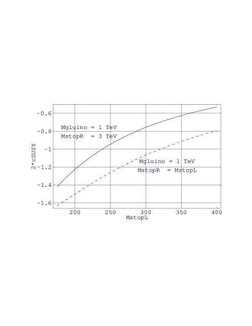
Figure 4: The quantity $2c^{\rm SUSY}$ as a function of the squark mass for $\tilde{M}_{g}=1$ TeV and $M_{t}=175$ GeV. Notice that the SUSY effects are negative.

3.2 Production cross section

3.2.1 Partonic Results

The hadronic cross section $\sigma_{hk}\equiv\sigma(hk\to\phi+X)$ for Higgs production can be written as

$$\begin{split}\sigma_{hk}(z)=\sum_{i,j}\int_{z}^{1}{\rm d}x_{1}\int_{z/x_{1}}^{1}{\rm d}x_{2}\,\,\varphi_{i/h}(x_{1})\,\varphi_{j/k}(x_{2})\,\hat{\sigma}_{ij}\left(\frac{z}{x_{1}x_{2}}\right)\,,\qquad z\equiv\frac{M_{\phi}^{2}}{s}\,,\end{split}$$ (30)

where $i$, $j$ denote any partons inside the hadrons $h$, $k$, and $\varphi(x)$ is a parton density. $\hat{\sigma}_{ij}$ is the partonic cross section, and $s$ is the hadronic c.m. energy

It is convenient to write this partonic cross section as

$$\begin{split}\hat{\sigma}_{ij}(x)=\sigma_{0}\,\Delta_{ij}(x)\,,\qquad x=\frac{M_{\phi}^{2}}{\hat{s}}\,,\qquad\sigma_{0}&=\frac{\pi^{2}}{8M_{\phi}^{3}}\Gamma_{0}\,,\end{split}$$ (31)

where $\Gamma_{0}$ is defined in Eq. (25), $\hat{s}$ is the partonic center-of-mass energy, and

$$\begin{split}\Delta_{ij}(x)=\delta_{ig}\delta_{jg}\,\delta(1-x)+\frac{\alpha_{s}}{\pi}\,\Delta_{ij}^{(1)}(x)+{\cal O}(\alpha_{s}^{2})\,.\end{split}$$ (32)

We find for the NLO terms ($q\in\{u,d,s,c\}$):

$$\begin{split}\Delta^{(1)}_{gg}&=\Delta^{(1),\rm SM}_{gg}+2\,c^{\rm SUSY}\,\delta(1-x)\,,\\[10.00002pt] \Delta^{(1),\rm SM}_{gg}&=\left(\frac{11}{2}+6\zeta_{2}\right)\delta(1-x)+12\left[\frac{\ln(1-x)}{1-x}\right]_{+}-12x(-x+x^{2}+2)\ln(1-x)\\ &\quad-\frac{6(x^{2}+1-x)^{2}}{1-x}\ln(x)-\frac{11}{2}(1-x)^{3}\,,\\ \Delta^{(1)}_{qg}&=\Delta^{(1),\rm SM}_{qg}=-\frac{2}{3}\left(1+(1-x)^{2}\right)\ln\frac{x}{(1-x)^{2}}-1+2x-\frac{1}{3}x^{2}\,,\\ \Delta^{(1)}_{q\bar{q}}&=\Delta^{(1),\rm SM}_{q\bar{q}}=\frac{32}{27}(1-x)^{3}\,,\end{split}$$ (33)

where $c^{\rm SUSY}$ is defined in Eq. (29) and the subscript “+” denotes the standard plus distribution. $\Delta^{\rm SM}_{ij}(x)$ is the NLO Standard Model expression [8, 9]. All other partonic subprocesses vanish at NLO. Note that the SUSY corrections only modify the coefficient of the $\delta(1-x)$ contribution in the gluonic channel.

3.2.2 Hadronic Results

Fig. 5 shows the NLO K-factor for hadronic Higgs production in the Standard Model and in Supersymmetry, for two different choices of squark and gluino masses, corresponding to the cases $(A)$ and $(B)$. We notice that, even though the overall normalization of the cross section in SUSY can be a multiple of the SM value, the QCD corrections are very similar in both cases, differing by less than 10%. However, in contrast to Ref. [17], we find that the SUSY effects are negative for large values of the gluino mass.

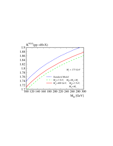
Figure 5: K-factors at NLO for Higgs production in gluon fusion in the Standard Model (dotted) and in Supersymmetry. Dashed line: $\tilde{M}_{R}=\tilde{M}_{L}=M_{t}=175$ GeV, $\tilde{M}_{g}=1$ TeV — Solid line: $\tilde{M}_{R}=1$ TeV, $\tilde{M}_{L}=M_{t}=175$ GeV, $\tilde{M}_{g}=400$ GeV. The bottom Yukawa coupling has been neglected. We use the LO and NLO parton densities of MRST2001 [37].

4 Conclusions

In this paper we considered the NLO supersymmetric corrections to the production and decay of a Higgs boson. We used the framework of an effective Lagrangian where the heavy particles enter the coefficient function, $C_{1}$, of the operator describing the gluon-Higgs coupling. The practical calculation is based on the evaluation of the gluon-Higgs vertex diagrams using asymptotic expansions. Our results are in disagreement with Ref. [17], which is due to the reasons that have been discussed above. The SUSY corrections decrease the effects from pure QCD by less than 5% in the considered parameter space. A more detailed numerical analysis and the inclusion of general squark mixing will be presented elsewhere.

Acknowledgments.

We are grateful to K. Chetyrkin, S. Heinemeyer, G. Kramer, A. Penin, and T. Plehn for discussions, T. Seidensticker for his help in the handling of q2e/exp, and G. Weiglein for discussions and useful comments to the manuscript. We would like to thank the authors of Ref. [17] for communications.

References

- [1]
- [2]
- [3] B. A. Kniehl, Phys. Rept. 240 (1994) 211.
- [4] M. Spira, Fortschr. Phys. 46 (1998) 203.
- [5] M. Carena and H.E. Haber, Prog. Part. Nucl. Phys. 50 (2003) 63.
- [6] D. Graudenz, M. Spira, and P.M. Zerwas, Phys. Rev. Lett. 70 (1993) 1372.
- [7] M. Spira, A. Djouadi, D. Graudenz, and P.M. Zerwas, Nucl. Phys. B 453 (1995) 17.
- [8] S. Dawson, Nucl. Phys. B 359 (1991) 283.
- [9] A. Djouadi, M. Spira, and P. M. Zerwas, Phys. Lett. B 264 (1991) 440.
- [10] R. V. Harlander and W. B. Kilgore, Phys. Rev. Lett. 88 (2002) 201801.
- [11] C. Anastasiou and K. Melnikov, Nucl. Phys. B 646 (2002) 220.
- [12] V. Ravindran, J. Smith, and W.L. van Neerven, hep-ph/0302135.
- [13] M. Spira, A. Djouadi, D. Graudenz, and P.M. Zerwas, Phys. Lett. B 318 (1993) 347.
-
[14]
E. Eichten, I. Hinchliffe, K. D. Lane, and C. Quigg,
Rev. Mod. Phys. 56 (1984) 579;
(E) 58 (1986) 1065. - [15] F. Maltoni, Z. Sullivan, and S. Willenbrock, Phys. Rev. D 67 (2003) 093005
- [16] R.V. Harlander and W.B. Kilgore, Phys. Rev. D 68 (2003) 013001.
- [17] S. Dawson, A. Djouadi, and M. Spira, Phys. Rev. Lett. 77 (1996) 16.
- [18] V. P. Spiridonov, IYaI-P-0378.
- [19] K. G. Chetyrkin, B. A. Kniehl, and M. Steinhauser, Nucl. Phys. B 510 (1998) 61.
- [20] T. Inami, T. Kubota, and Y. Okada, Z. Phys. C 18 (1983) 69.
- [21] K. G. Chetyrkin, B. A. Kniehl, and M. Steinhauser, Phys. Rev. Lett. 79 (1997) 353.
- [22] M. Krämer, E. Laenen, and M. Spira, Nucl. Phys. B 511 (1998) 523.
- [23] G. ’t Hooft and M. J. Veltman, Nucl. Phys. B 44 (1972) 189.
- [24] W. Siegel, Phys. Lett. B 84 (1979) 193.
- [25] I. Jack and D. R. Jones, hep-ph/9707278.
- [26] P. Nogueira, J. Comp. Phys. 105 (1993) 279.
- [27] T. Seidensticker, unpublished.
-
[28]
T. Seidensticker,
hep-ph/9905298;
R. Harlander, T. Seidensticker, and M. Steinhauser, Phys. Lett. B 426 (1998) 125. - [29] M. Steinhauser, Comp. Phys. Commun. 134 (2001) 335.
- [30] S.A. Larin, F.V. Tkachov, and J.A. Vermaseren, NIKHEF-H-91-18.
- [31] K.G. Chetyrkin and F.V. Tkachov, Nucl. Phys. B 192 (1981) 159.
- [32] M. Steinhauser, Phys. Reports 364 (2002) 247.
-
[33]
S. Kraml,
hep-ph/9903257;
H. Eberl, Dissertation, TU Wien, 1998. - [34] V. A. Smirnov, Applied Asymptotic Expansions in Momenta and Masses, (Springer-Verlag, Heidelberg, 2001).
- [35] R. Harlander and M. Steinhauser, Prog. Part. Nucl. Phys. 43 (1999) 167.
- [36] T. Appelquist and J. Carazzone, Phys. Rev. D 11 (1975) 2856.
- [37] A. D. Martin, R. G. Roberts, W. J. Stirling, and R. S. Thorne, Eur. Phys. J. C 23 (2002) 73.