hep-ph/0307344 PITHA 03/05
  LMU 16/03
  FERMILAB-Pub-03/214-T
  July 2003

CP asymmetry in flavour-specific B decays

beyond leading logarithms

Martin Beneke¹,  Gerhard Buchalla²,

Alexander Lenz³  and  Ulrich Nierste⁴

¹ Institut für Theoretische Physik E, RWTH Aachen, Sommerfeldstraße 28,
¹ D-52074 Aachen, Germany.
² Ludwig-Maximilians-Universität München, Sektion Physik, Theresienstraße 37,
¹ D-80333 München, Germany.
³ Fakultät für Physik, Universität Regensburg, D-93040 Regensburg, Germany.
⁴ Fermi National Accelerator Laboratory, Batavia, IL 60510-500, USA.

Abstract

We compute next-to-leading order QCD corrections to the CP asymmetry $a_{\rm fs}={\rm Im}(\Gamma_{12}/M_{12})$ in flavour-specific $B_{d,s}$ decays such as $B_{d}\to X\ell\overline{\nu}_{\ell}$ or $B_{s}\to D_{s}^{-}\pi^{+}$. The corrections reduce the uncertainties associated with the choice of the renormalization scheme for the quark masses significantly. In the Standard Model we predict $a^{d}_{\rm fs}=-(5.0\pm 1.1)\times 10^{-4}$. As a by-product we also obtain the width difference in the $B_{d}$ system at next-to-leading order in QCD.

PACS numbers: 11.30.Er, 12.38.Bx, 13.25.Hw, 14.40.Nd
Keywords: asymmetry, CP; B0 anti-B0, mixing angle; B/s0, semileptonic decay

1 Preliminaries

$B_{d}$ and $B_{s}$ mesons mix with their antiparticles. The time evolution of the $B_{q}\!-\!\,\overline{\!B}{}_{q}\,$ system (with $q=d$ or $s$) is characterized by two hermitian $2\times 2$ matrices, the mass matrix $M^{q}$ and the decay matrix $\Gamma^{q}$. The oscillations between the flavour eigenstates $B_{q}$ and $\,\overline{\!B}_{q}$ involve the three physical quantities $|M_{12}^{q}|$, $|\Gamma_{12}^{q}|$ and $\phi_{q}=\arg(-M_{12}^{q}/\Gamma_{12}^{q})$ (see e.g. [1]). They are related to the mass and width differences of the $B_{q}$ system as

$$\Delta M_{q} = 2\,|M_{12}^{q}|,\qquad\Delta\Gamma_{q}\;=\;\Gamma^{q}_{L}-\Gamma^{q}_{H}\;=\;2\,|\Gamma_{12}^{q}|\cos\phi_{q},$$ (1)

where $\Gamma^{q}_{L}$ and $\Gamma^{q}_{H}$ denote the widths of the lighter and heavier mass eigenstate, respectively. Here and in the following we neglect tiny corrections of order $|\Gamma_{12}^{q}/M_{12}^{q}|^{2}$.

The CP-violating phase $\phi_{q}$ can be measured through the CP asymmetry $a_{\rm fs}^{q}$ in flavour-specific $B_{q}\to f$ decays, which means that the decays $\,\overline{\!B}_{q}\to f$ and $B_{q}\to\overline{f}$ are forbidden [2]:

$$a^{q}_{\rm fs} = \frac{\Gamma(\,\overline{\!B}{}_{q}(t)\rightarrow f)-\Gamma(B_{q}(t)\rightarrow\overline{f})}{\Gamma(\,\overline{\!B}{}_{q}(t)\rightarrow f)+\Gamma(B_{q}(t)\rightarrow\overline{f})}\;=\;\mathrm{Im}\,\frac{\Gamma_{12}^{q}}{M_{12}^{q}}\;=\;\frac{\Delta\Gamma_{q}}{\Delta M_{q}}\tan\phi_{q}.$$ (2)

Here $B_{q}(t)$ and $\,\overline{\!B}{}_{q}(t)$ denote mesons which are tagged as a $B_{q}$ and $\,\overline{\!B}_{q}$ at time $t=0$, respectively. An additional requirement in Eq. (2) is the absence of direct CP violation in $B_{q}\to f$, which is equivalent to $|\langle f|B_{q}\rangle|=|\langle\overline{f}|\,\overline{\!B}_{q}\rangle|$. For example, $a_{\rm fs}^{s}$ can be obtained through $B_{s}\to D_{s}^{-}\pi^{+}$. The standard way to access $a_{\rm fs}^{q}$ uses $B_{q}\to X\ell^{-}\overline{\nu_{\ell}}$ decays, which justifies the name semileptonic CP asymmetry for $a_{\rm fs}^{q}$. The measurement of $a^{q}_{\rm fs}$ does not require tagging (see e.g. [3]). A further method to access $a^{q}_{\rm fs}$ uses the fully inclusive, tagged $B$ decay asymmetry discussed in [4].

$a_{\rm fs}^{q}$ is small because of two suppression factors: First $|\Gamma_{12}/M_{12}|=O(m_{b}^{2}/M_{W}^{2})$ suppresses $a_{\rm fs}^{q}$ to the percent level. Second there is a GIM suppression factor $m_{c}^{2}/m_{b}^{2}$ reducing $a_{\rm fs}^{q}$ by another order of magnitude. This GIM suppression is lifted if new physics contributes to $\arg M_{12}$. Therefore $a_{\rm fs}^{q}$ is very sensitive to new CP phases [1, 5]. Up to now, the Standard Model (SM) prediction for $a_{\rm fs}^{q}$ was only known in the leading-logarithmic approximation. The unknown next-to-leading order (NLO) QCD corrections were identified as the largest theoretical uncertainty in $a^{q}_{\rm fs}$ [5]. While NLO corrections were calculated long ago for $M_{12}^{q}$ [6], only certain portions of the QCD corrections to $\Gamma_{12}^{q}$ (relevant to $\Delta\Gamma_{s}$) were known so far [7]. In Sect. 2 we compute the missing pieces of the latter. Predictions for $a_{\rm fs}^{q}$ and $\Delta\Gamma_{d}$ can be found in Sect. 3.

2 $\Gamma_{12}^{q}$ at next-to-leading order in QCD

Figure 1: Leading order contribution to $\Gamma_{12}$ (left) and a sample NLO diagram (right). The crosses denote effective $\Delta B=1$ operators triggering the $b$ decay. The full set of NLO diagrams can be found in [7].

In this section we specify the discussion to the case $q=d$ and omit the index $q$. The generalization of our results to $\Gamma_{12}^{s}$ is straightforward. $\Gamma_{12}$ is an inclusive quantity stemming from decays into final states common to $B$ and $\,\overline{\!B}$. It can be computed with the help of the heavy quark expansion (HQE) [8] from diagrams like those in Figure 1. The HQE is a simultaneous expansion in $\Lambda_{\rm QCD}/m_{b}$ and $\alpha_{s}(m_{b})$. Corrections of order $\Lambda_{\rm QCD}/m_{b}$ to $\Gamma_{12}$ have been calculated in [9, 10] and applied to $a_{\rm fs}$ in [5].

We decompose $\Gamma_{12}$ as

$$\Gamma_{12} = -\left[\,\lambda_{c}^{2}\,\Gamma_{12}^{cc}\;+\;2\,\lambda_{c}\,\lambda_{u}\,\Gamma_{12}^{uc}\;+\;\lambda_{u}^{2}\,\Gamma_{12}^{uu}\,\right]$$ (3)

with the CKM factors $\lambda_{i}=V_{id}^{*}V_{ib}$ for $i=u,c,t$. The coefficients $\Gamma_{12}^{ab}$, $a,b=u,c$ in Eq. (3), which are computed from diagrams like those in Figure 1, are positive. We present the new NLO expressions for the coefficient $\Gamma_{12}^{uc}$ in the appendix. $\Gamma_{12}^{cc}$ has already been given at NLO in [7], and $\Gamma_{12}^{uu}$ can be inferred by taking the limit $z\to 0$ in $\Gamma_{12}^{cc}$. It is convenient to write

$$\frac{\Gamma_{12}}{M_{12}} = \frac{\lambda_{t}^{2}}{M_{12}}\left[-\Gamma_{12}^{cc}\;+\;\,2\,\left(\Gamma_{12}^{uc}\,-\,\Gamma_{12}^{cc}\right)\,\frac{\lambda_{u}}{\lambda_{t}}\;+\;\left(2\,\Gamma_{12}^{uc}\,-\,\Gamma_{12}^{cc}\,-\,\Gamma_{12}^{uu}\right)\,\frac{\lambda_{u}^{2}}{\lambda_{t}^{2}}\right]$$ (4)

$$=\,10^{-4}\left[\,c_{1}+c_{2}\frac{B_{S}^{\prime}}{B}+c_{m}\;+\;\left(a_{1}+a_{2}\frac{B_{S}^{\prime}}{B}+a_{m}\right)\,\frac{\lambda_{u}}{\lambda_{t}}\;+\;\left(b_{1}+b_{2}\frac{B_{S}^{\prime}}{B}+b_{m}\right)\,\frac{\lambda_{u}^{2}}{\lambda_{t}^{2}}\,\right].$$

Here $B=B(\mu_{2}=m_{b})$ and $B_{S}^{\prime}=B_{S}^{\prime}(\mu_{2}=m_{b})$ parameterize the hadronic matrix elements of the local $\Delta B\!=\!2$ operators $Q$ and $Q_{S}$:

$$Q = \overline{q}\gamma_{\mu}(1-\gamma_{5})b\,\overline{q}\gamma^{\mu}(1-\gamma_{5})b,\qquad Q_{S}\;=\;\overline{q}(1+\gamma_{5})b\,\overline{q}(1+\gamma_{5})b,$$

$$\langle B_{d}|Q(\mu_{2})|\overline{B}{}_{d}\rangle = \frac{8}{3}f_{B_{d}}^{2}M_{B_{d}}^{2}B(\mu_{2}),$$

$$\langle B_{d}|Q_{S}(\mu_{2})|\overline{B}{}_{d}\rangle = -\frac{5}{3}f_{B_{d}}^{2}M_{B_{d}}^{2}B_{S}^{\prime}(\mu_{2})\;=\;-\frac{5}{3}f_{B_{d}}^{2}M_{B_{d}}^{2}\frac{M_{B_{d}}^{2}}{\left[\overline{m}_{b}(\mu_{2})+\overline{m}_{d}(\mu_{2})\right]^{2}}B_{S}(\mu_{2}).$$ (5)

The mass $M_{B_{d}}$ and decay constant $f_{B_{d}}$ cancel from Eq. (4). $B$ and $B_{S}^{\prime}$ depend on the scale $\mu_{2}$ and the renormalization scheme used in the computation of the matrix elements in Eq. (5). When combining values for $B_{S}^{\prime}/B$ with our results for $c_{1,2}$, $a_{1,2}$ and $b_{1,2}$ below, one must verify that they correspond to the same scheme. Details on the renormalization scheme used by us can be found in [7]. Often the parameter $B_{S}$ rather than $B_{S}^{\prime}$ is chosen to parameterize $\langle Q_{S}\rangle$. As shown in Eq. (5), they differ by a factor involving $\overline{\rm MS}$ masses. $\overline{m}_{b}(\overline{m}_{b})$ is smaller than the pole mass $m_{b}$ by roughly 0.4 GeV.

For the evaluation of Eq. (4) we also need the SM prediction for $M_{12}$:

$$M_{12} = \lambda_{t}^{2}\,\frac{G_{F}^{2}}{12\pi^{2}}M_{B_{d}}\,\eta_{B}\,B(\mu_{2})b_{B}(\mu_{2})f_{B_{d}}^{2}\,M_{W}^{2}S\left(\frac{\overline{m}_{t}^{2}}{M_{W}^{2}}\right)$$ (6)

with the QCD factors $\eta_{B}=0.55$ [6] and

$$b_{B}(\mu) = \left[\alpha_{s}(\mu)\right]^{-6/23}\,\left[1+\frac{\alpha_{s}(\mu)}{4\pi}\frac{5165}{3174}\right],\qquad\quad b_{B}(m_{b})\;=\;1.52\pm 0.03.$$

Note that results from lattice gauge theory are often quoted for the scale and scheme invariant parameter $\widehat{B}=b_{B}(\mu_{2})B(\mu_{2})$ rather than $B(m_{b})$ entering Eq. (4).

We use the following input for the physical parameters (where $\overline{m}_{i}\equiv\overline{m}_{i}(\overline{m}_{i})$):

$$\overline{m}_{b} = (4.25\pm 0.08)\,\mbox{GeV},\qquad\overline{m}_{c}\;=\;(1.30\pm 0.05)\,\mbox{GeV},$$

$$\alpha_{s}(M_{Z}) = 0.118\pm 0.003,\qquad\qquad\overline{m}_{t}\;=\;(167\pm 5)\,\mbox{GeV},$$

$$B_{S}^{\prime}/B = 1.4\pm 0.2,\hskip 69.99396ptm_{b}^{\rm pow}\;=\;(4.8\pm 0.2)\,\mbox{GeV}.$$ (7)

The top mass mainly enters the result through $S(\overline{m}_{t}^{2}/M_{W}^{2})$ in Eq. (6), which evaluates to $S(\overline{m}_{t}^{2}/M_{W}^{2})=2.40\pm 0.11$. In the power corrections $a_{m}$, $b_{m}$, $c_{m}$ the renormalization scheme is not fixed, because corrections of order $\alpha_{s}/m_{b}$ are unknown. The expansion parameter of the HQE is the pole mass and we use $m_{b}^{\rm pow}=4.8\pm 0.2\,\mbox{GeV}$ (and $m_{d}=7\,{\rm MeV}$) in $a_{m}$, $b_{m}$ and $c_{m}$. For the determination of

$$a = a_{1}+a_{2}\frac{B_{S}^{\prime}}{B}+a_{m}$$ (8)

and the analogously defined quantities $b$ and $c$ we take $B_{S}^{\prime}/B=1.4\pm 0.2$, which covers the range of recent lattice computations [12]. We estimate the accuracy of our calculation by computing the coefficients in two schemes for the quark masses (pole and $\overline{\rm MS}$), as explained in the appendix. Further we vary the renormalization scale $\mu_{1}$ between one half and twice the $b$ quark mass in the corresponding scheme. The result is shown in Figure 2 for the coefficient $a$, which is most relevant to $a_{\rm fs}$: While the dependence on $\mu_{1}$ is small in both LO and NLO, the scheme dependence is huge in LO and reduced by roughly a factor of 4 in NLO. We quote our coefficients for the two schemes and add the errors from Eq. (7), and the uncertainty from the $\mu_{1}$-dependence in quadrature:

$$\begin{array}[b]{r|r@{\qquad}r@{\qquad}r@{\qquad}r@{\qquad}r}&\mbox{LO, $\overline{\rm MS}$}&\mbox{LO, pole}&\mbox{NLO, $\overline{\rm MS}$}&\mbox{NLO, pole}\\ \hline\cr\\[-5.69054pt] a_{1}&6.75\raisebox{-2.15277pt}{\shortstack[l]{$\scriptstyle+0.89$\\ $\scriptstyle-0.89$}}&13.96\raisebox{-2.15277pt}{\shortstack[l]{$\scriptstyle+1.12$\\ $\scriptstyle-1.10$}}&8.32\raisebox{-2.15277pt}{\shortstack[l]{$\scriptstyle+1.24$\\ $\scriptstyle-1.23$}}&10.45\raisebox{-2.15277pt}{\shortstack[l]{$\scriptstyle+0.93$\\ $\scriptstyle-0.91$}}\\[5.69054pt] a_{2}&0.92\raisebox{-2.15277pt}{\shortstack[l]{$\scriptstyle+0.31$\\ $\scriptstyle-0.28$}}&4.77\raisebox{-2.15277pt}{\shortstack[l]{$\scriptstyle+1.16$\\ $\scriptstyle-1.04$}}&1.36\raisebox{-2.15277pt}{\shortstack[l]{$\scriptstyle+0.41$\\ $\scriptstyle-0.37$}}&1.86\raisebox{-2.15277pt}{\shortstack[l]{$\scriptstyle+1.36$\\ $\scriptstyle-1.34$}}\\[5.69054pt] b_{1}&-0.03\raisebox{-2.15277pt}{\shortstack[l]{$\scriptstyle+0.01$\\ $\scriptstyle-0.02$}}&-0.31\raisebox{-2.15277pt}{\shortstack[l]{$\scriptstyle+0.08$\\ $\scriptstyle-0.10$}}&0.00\raisebox{-2.15277pt}{\shortstack[l]{$\scriptstyle+0.02$\\ $\scriptstyle-0.02$}}&0.10\raisebox{-2.15277pt}{\shortstack[l]{$\scriptstyle+0.17$\\ $\scriptstyle-0.17$}}\\[5.69054pt] b_{2}&0.09\raisebox{-2.15277pt}{\shortstack[l]{$\scriptstyle+0.04$\\ $\scriptstyle-0.03$}}&0.80\raisebox{-2.15277pt}{\shortstack[l]{$\scriptstyle+0.26$\\ $\scriptstyle-0.22$}}&0.08\raisebox{-2.15277pt}{\shortstack[l]{$\scriptstyle+0.05$\\ $\scriptstyle-0.04$}}&0.00\raisebox{-2.15277pt}{\shortstack[l]{$\scriptstyle+0.34$\\ $\scriptstyle-0.34$}}\\[5.69054pt] c_{1}&-6.60\raisebox{-2.15277pt}{\shortstack[l]{$\scriptstyle+2.31$\\ $\scriptstyle-2.32$}}&-2.01\raisebox{-2.15277pt}{\shortstack[l]{$\scriptstyle+3.03$\\ $\scriptstyle-3.03$}}&-3.61\raisebox{-2.15277pt}{\shortstack[l]{$\scriptstyle+1.32$\\ $\scriptstyle-1.33$}}&-1.01\raisebox{-2.15277pt}{\shortstack[l]{$\scriptstyle+1.08$\\ $\scriptstyle-1.08$}}\\[5.69054pt] c_{2}&-54.65\raisebox{-2.15277pt}{\shortstack[l]{$\scriptstyle+7.20$\\ $\scriptstyle-7.28$}}&-61.12\raisebox{-2.15277pt}{\shortstack[l]{$\scriptstyle+8.08$\\ $\scriptstyle-8.17$}}&-45.54\raisebox{-2.15277pt}{\shortstack[l]{$\scriptstyle+3.67$\\ $\scriptstyle-3.77$}}&-40.41\raisebox{-2.15277pt}{\shortstack[l]{$\scriptstyle+6.52$\\ $\scriptstyle-6.56$}}\\[5.69054pt] a_{m}&0.11\raisebox{-2.15277pt}{\shortstack[l]{$\scriptstyle+0.06$\\ $\scriptstyle-0.06$}}&0.63\raisebox{-2.15277pt}{\shortstack[l]{$\scriptstyle+0.31$\\ $\scriptstyle-0.30$}}&0.11\raisebox{-2.15277pt}{\shortstack[l]{$\scriptstyle+0.06$\\ $\scriptstyle-0.06$}}&0.65\raisebox{-2.15277pt}{\shortstack[l]{$\scriptstyle+0.32$\\ $\scriptstyle-0.31$}}\\[5.69054pt] b_{m}&0.03\raisebox{-2.15277pt}{\shortstack[l]{$\scriptstyle+0.02$\\ $\scriptstyle-0.02$}}&0.23\raisebox{-2.15277pt}{\shortstack[l]{$\scriptstyle+0.12$\\ $\scriptstyle-0.11$}}&0.03\raisebox{-2.15277pt}{\shortstack[l]{$\scriptstyle+0.02$\\ $\scriptstyle-0.02$}}&0.24\raisebox{-2.15277pt}{\shortstack[l]{$\scriptstyle+0.12$\\ $\scriptstyle-0.12$}}\\[5.69054pt] c_{m}&22.08\raisebox{-2.15277pt}{\shortstack[l]{$\scriptstyle+9.06$\\ $\scriptstyle-9.40$}}&21.93\raisebox{-2.15277pt}{\shortstack[l]{$\scriptstyle+8.95$\\ $\scriptstyle-9.29$}}&22.45\raisebox{-2.15277pt}{\shortstack[l]{$\scriptstyle+9.22$\\ $\scriptstyle-9.57$}}&22.32\raisebox{-2.15277pt}{\shortstack[l]{$\scriptstyle+9.12$\\ $\scriptstyle-9.46$}}\\ \end{array}$$ (9)

In the case of $a_{m},\ldots,c_{m}$ the difference between the LO and NLO columns stems solely from the QCD factor $\eta_{B}$. The reduction of the scheme dependence of $a_{1},\ldots,c_{2}$ is evident from the comparison of the last two columns with the first two ones.

Our final values for $a$, $b$, and $c$ are at NLO (LO results in parentheses):

$$a = {12.0\pm 2.4}\hskip 12.6152pt\qquad\quad(14.7\pm 6.7)$$

$$b = {0.2\pm 0.1}\hskip 17.13603pt\qquad\quad(0.6\pm 0.5)$$

$$c = -40.1\pm 15.8\qquad\quad(-63.3\pm 15.6)$$ (10)

They have been obtained by averaging the results in the pole scheme and the $\overline{\rm MS}$ scheme for central values of the input parameters. The error from scheme dependence was taken to be half the difference between the results in the two schemes. The errors quoted in Eq. (10) were obtained by combining in quadrature the latter error with the uncertainties in the $\overline{\rm MS}$ scheme from scale dependence ($\mu_{1}$), $\overline{m}_{c}$, $\overline{m}_{b}$, $\overline{m}_{t}$, $\alpha_{s}(M_{Z})$, $B^{\prime}_{S}/B$, and the $b$-mass in the power corrections.

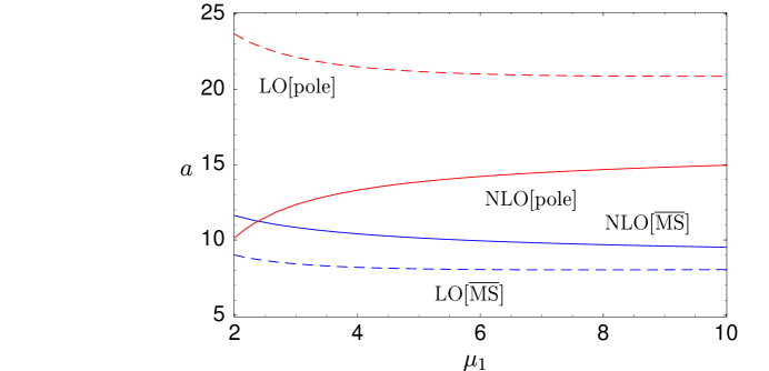
Figure 2: Dependence of $a$ on the scale $\mu_{1}$. The solid (dashed) lines show the NLO (LO) results.

In order to understand the size of the coefficients $a$, $b$, $c$ at leading and next-to-leading order and the impact of various uncertainties, it is instructive to expand in the small parameter $z=m^{2}_{c}/m^{2}_{b}\sim 0.1$. The leading terms in this expansion behave as follows:

$$\begin{array}[]{r|c|c|c|c|c|c|c}&a_{1}&a_{2}&b_{1},b_{2}&c_{1},c_{2}&a_{m}&b_{m}&c_{m}\\ \hline\cr&&&&&&&\\[-5.69054pt] {\rm LO}&z&z^{2}&z^{3}&1&z^{2}&z^{3}&1\\[5.69054pt] \hline\cr&&&&&&&\\[-5.69054pt] {\rm NLO}&\ \alpha_{s}z,\alpha_{s}z\ln z&\ \alpha_{s}z&\ \alpha_{s}z^{2}&\ \alpha_{s}&-&-&-\end{array}$$ (11)

Here we have displayed the coefficients $a_{i}$, $b_{i}$ and $c_{i}$ separately, indicating the leading order terms and the NLO corrections.

In the SM the CP asymmetry $a_{\rm fs}$ does not depend on $c_{i}$, but only on $a_{i}$ and $b_{i}$, on which we shall focus for the moment. Both $a$ and $b$ exhibit an interesting pattern of GIM suppression, which leads to a pronounced hierarchy among the different contributions. All of the coefficients of $a_{\rm fs}$ have to vanish as $z\to 0$. The dominant term is $a_{1}$, while $a_{2}$ is suppressed by one, $b_{1,2}$ even by two additional powers of $z$ at LO. This strong hierarchy is alleviated at NLO, where the $z^{2}$ and $z^{3}$ terms receive corrections of order $\alpha_{s}z$ and $\alpha_{s}z^{2}$. Hence they are still parametrically smaller than $a_{1}$, which remains the most important coefficient. As a consequence of this pattern, the coefficients $b_{1,2}$ get larger relative corrections at NLO, but remain strongly suppressed in comparison to $a_{1}$. This suppression is also not changed by the power corrections $b_{m}$. Thus $b$ has only a minor impact on $a_{\rm fs}$. An additional welcome feature is the suppression of $a_{2}$, which considerably reduces the dependence on the hadronic matrix elements $B^{\prime}_{S}/B$. We emphasize that the dominant term $a_{1}$ is free of hadronic uncertainties since the matrix element $B$ in $\Gamma_{12}$ cancels against the identical quantity in $M_{12}$. It can be seen from Eq. (11) that power corrections to $a$ are suppressed by an additional factor of $z$. As a result of all these properties, $a_{\rm fs}$ is quite accurately known in the SM, once the NLO QCD effects are taken into account. Note that the latter are important to eliminate the sizable scheme ambiguity of the leading order calculation. We remark that the $\alpha_{s}z\ln z$ term in $a_{1}$ is peculiar to the choice of pole masses $z=m^{2}_{c,pole}/m^{2}_{b,pole}$, which at one-loop order is equivalent to $z=\overline{m}^{2}_{c}(\overline{m}_{c})/\overline{m}^{2}_{b}(\overline{m}_{b})$. Expressing the results in terms of $\overline{z}=\overline{m}^{2}_{c}(\overline{m}_{b})/\overline{m}^{2}_{b}(\overline{m}_{b})$, the $z\ln z$ term is eliminated. As discussed in [11] the absence of these terms holds to all orders in $\alpha_{s}$. Finally, at NLO the overall uncertainty in $a$ and $b$ comes predominantly from $\overline{m}_{c}$ and from the residual scheme dependence.

The situation is different for $c$, which is enhanced relative to $a$, $b$. Here sizable uncertainties are still present at NLO from the dependence on $B^{\prime}_{S}/B$, power corrections and, to a lesser extent, also from residual scale and scheme dependence. The parameter $c$ enters the width difference $\Delta\Gamma_{d}$ and, in general, the expression for $a_{\rm fs}$ in the presence of new physics. In these cases one has larger theoretical uncertainties than in the SM analysis of $a_{\rm fs}$.

3 Phenomenology

In the SM the CP asymmetry for the $B_{d}$ system reads

$$a_{\rm fs}^{d}\;=\;\mathrm{Im}\,\frac{\Gamma_{12}}{M_{12}} = \left[\,a\,\mathrm{Im}\,\frac{\lambda_{u}}{\lambda_{t}}\;+\;b\,\mathrm{Im}\,\frac{\lambda_{u}^{2}}{\lambda_{t}^{2}}\,\right]\,10^{-4},$$ (12)

where $a$ and $b$ are given in Eq. (10). In terms of Wolfenstein parameters $\bar{\rho}$ and $\bar{\eta}$ the CKM quantities in Eq. (12) are

$$\frac{\lambda_{u}}{\lambda_{t}}=\frac{1-\bar{\rho}-i\bar{\eta}}{(1-\bar{\rho})^{2}+\bar{\eta}^{2}}-1=\frac{\cos\beta-i\sin\beta}{R_{t}}-1$$ (13)

$${\rm Im}\frac{\lambda_{u}}{\lambda_{t}}=-\frac{\sin\beta}{R_{t}}\,,\qquad\qquad{\rm Im}\left(\frac{\lambda_{u}}{\lambda_{t}}\right)^{2}=\frac{2\sin\beta}{R_{t}}-\frac{\sin 2\beta}{R^{2}_{t}}$$ (14)

where $\beta=\arg(-\lambda_{t}/\lambda_{c})$ and $R_{t}\equiv\sqrt{(1-\bar{\rho})^{2}+\bar{\eta}^{2}}$ are one angle and one side of the usual unitarity triangle.

A future measurement of $a^{d}_{\rm fs}$ will allow us to constrain $\bar{\rho}$ and $\bar{\eta}$ within the SM using the theoretical values for $a$ and $b$. This is illustrated in Figure 3.

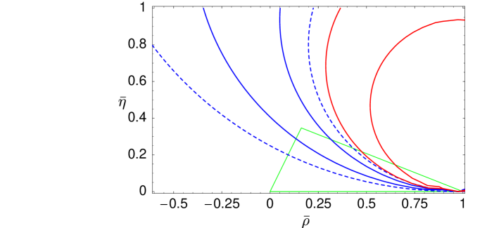
Figure 3: Constraints in the ($\bar{\rho},\bar{\eta}$) plane implied by given values of the CP asymmetry $a^{d}_{\rm fs}$. The area between the solid pair of curves on the right represents the theoretical uncertainty at NLO, assuming $a^{d}_{\rm fs}=-10^{-3}$. Similarly, the curves on the left indicate the uncertainty for $a^{d}_{\rm fs}=-5\times 10^{-4}$ both at NLO (solid) and at LO (dashed). The currently favoured solution for the unitarity triangle is also shown.

Using Eq. (10) and [13]

$$R_{t}=0.91\pm 0.05\,,\qquad\qquad\beta=(22.4\pm 1.4)^{\circ}$$ (15)

we predict for $a^{d}_{\rm fs}$ in the SM

$$a^{d}_{\rm fs}=-(5.0\pm 1.1)\times 10^{-4}$$ (16)

This result is entirely dominated by the $a$-term in Eq. (12) since the small contribution from $b$ is further suppressed by its CKM coefficient, which is small for standard CKM parameters.

Our results can also be applied to the case of $B_{s}$ mesons, where Eq. (12) holds with obvious replacements. Here the term proportional to $b$ is strongly CKM suppressed and can be neglected. $SU(3)$ breaking in $a$ is negligible as well and the result in Eq. (10) may be used. We then find ($V_{us}=0.222$)

$$a^{s}_{\rm fs}=a|V_{us}|^{2}R_{t}\sin\beta\,\times 10^{-4}={(0.21\pm 0.04)\times 10^{-4}}$$ (17)

The width difference in the $B_{d}$ system is given by $\Delta\Gamma_{d}/\Delta M_{d}=-{\rm Re}(\Gamma_{12}/M_{12})$. The real part of $\Gamma_{12}/M_{12}$ can be found using Eqs. (4), (10), (13) and (15). It turns out that for the parameters in Eq. (15) the $c$-term yields the full result to within about $2\%$. In view of the large uncertainty of $c$, the contributions from $a$ and $b$ can be safely neglected. We then obtain the SM prediction

$$\frac{\Delta\Gamma_{d}}{\Delta M_{d}}=(4.0\pm 1.6)\times 10^{-3}\,,\qquad\qquad\frac{\Delta\Gamma_{d}}{\Gamma_{d}}=(3.0\pm 1.2)\times 10^{-3}$$ (18)

where the second expression follows with the experimental value $\Delta M_{d}/\Gamma_{d}=0.755$. This result for $\Delta\Gamma_{d}/\Gamma_{d}$ is in agreement with [1, 10]. To the extent that $SU(3)$ breaking in the ratio of bag factors $B^{\prime}_{S}/B$ can be neglected, the number for $\Delta\Gamma/\Delta M$ in Eq. (18) applies to the $B_{s}$ system as well.

The effects of new physics in $M_{12}$ on $a^{d}_{\rm fs}$ have been discussed in [5]. If magnitude and phase of $M_{12}$ are parameterized as

$$M_{12}=r^{2}_{d}e^{2i\theta_{d}}M^{\rm SM}_{12}$$ (19)

one obtains [5]

$$a^{d}_{\rm fs}=-{\rm Re}\left(\frac{\Gamma_{12}}{M_{12}}\right)_{\rm SM}\frac{\sin 2\theta_{d}}{r^{2}_{d}}+{\rm Im}\left(\frac{\Gamma_{12}}{M_{12}}\right)_{\rm SM}\frac{\cos 2\theta_{d}}{r^{2}_{d}}$$ (20)

Since the real part of $\Gamma_{12}/M_{12}$ in the SM is much larger than the imaginary part, $a_{\rm fs}$ is particularly sensitive to new physics. In this more general context our results can also be used. However, it has to be kept in mind that the SM analysis leading to Eq. (15) may no longer be true in the presence of new physics and the determination of CKM quantities then needs to be modified.

To summarize, we have computed the CP violating observables $a^{q}_{\rm fs}$ at next-to-leading order in QCD. We include the effect of penguin operators in the weak Hamiltonian and the power corrections of relative order $\Lambda_{QCD}/m_{b}$. Our SM predictions are given in Eqs. (16) and (17). We emphasize that within the heavy-quark expansion the $a^{q}_{\rm fs}$ can be reliably computed in the SM as functions of CKM parameters. A crucial element is the small sensitivity to hadronic parameters, which enter only as the ratio $B^{\prime}_{S}/B$ and only with a suppression factor of $z=(m_{c}/m_{b})^{2}$. After including the NLO corrections, the theoretical error on $a^{q}_{\rm fs}$ is reduced to about $20\%$. This is largely due to a reduction of the scheme ambiguity in the definition of quark masses by a factor of 4 in comparison with the LO result. The remaining uncertainty is larger for $\Delta\Gamma_{q}$. The result at next-to-leading order in QCD is given in Eq. (18). The measurement of $a^{q}_{\rm fs}$ is possible using suitable flavour-specific decay modes of neutral $B$ mesons. If it can be performed with sufficient accuracy, it will provide a significant test of the Standard Model. The large sensitivity of $a^{q}_{\rm fs}$ to new physics is reinforced by the improved theoretical analysis presented here.

Note added

The topic of this paper has also been addressed by Ciuchini et al. [14], who pointed out an error in an earlier preprint version of this paper. Our analytical results in Eq. (25) now agree with those in Eqs. (43-45) of [14]. We thank the authors of [14] for clarifying communication.

Acknowledgement

The work of M.B. is supported in part by the Bundesministerium für Bildung und Forschung, Project 05 HT1PAB/2, and by the DFG Sonderforschungsbereich/Transregio 9 “Computer-gestützte Theoretische Teilchenphysik”.

Appendix A NLO coefficients

Here we collect more detailed results for the coefficients in Eq. (3). The HQE expresses $\Gamma_{12}^{ab}$ for the $B_{d}$ system as

$$\Gamma_{12}^{ab} = \frac{G_{F}^{2}m_{b}^{2}}{24\pi}f_{B_{d}}^{2}M_{B_{d}}\left[\left(F^{ab}(z)+P^{ab}(z)\right)\frac{8}{3}B-\left(F_{S}^{ab}(z)+P_{S}^{ab}(z)\right)\frac{5}{3}B_{S}^{\prime}\right]+\Gamma_{12,1/m_{b}}^{ab}.$$ (21)

The short-distance coefficients $F^{ab}(z)$ contain the contributions from the $\Delta B\!=\!1$ current-current operators $Q_{1}$ and $Q_{2}$. The NLO results for $F^{cc}(z)$ and $F_{S}^{cc}(z)$ have been derived in [7], where these coefficients are called $F(z)$ and $F_{S}(z)$, respectively. Further $F^{uu}=F^{cc}(0)$ and $F_{S}^{uu}=F_{S}^{cc}(0)$. The coefficients $P(z)$ and $P_{S}(z)$ contain the contributions from penguin operators. They come with small coefficients, which simplifies the NLO calculation [7].

Our new calculation concerns $F^{uc}$, $F_{S}^{uc}$, $P^{uc}$ and $P_{S}^{uc}$. We decompose $F^{uc}$ and $F_{S}^{uc}$ as in [7, 11]:

$$F^{uc}(z) = C_{1}^{2}F_{11}^{uc}(z)+C_{1}C_{2}F_{12}^{uc}(z)+C_{2}^{2}F_{22}^{uc}(z),$$

$$F_{ij}^{uc}(z) = F_{ij}^{uc,(0)}(z)+\frac{\alpha_{s}(\mu_{1})}{4\pi}F_{ij}^{uc,(1)}(z,x_{\mu_{1}},x_{\mu_{2}})+{\cal O}(\alpha_{s}^{2})$$ (22)

with $x_{\mu}=\mu/m_{b}$ and an analogous notation for $F_{S,ij}^{uc}$. The $\Delta B\!=\!n$ operators, $n=1,2$, are defined at the scale $\mu_{n}={\cal O}(m_{b})$. The dependence of $F_{ij}^{uc}$ on $\mu_{1}$ diminishes order-by-order in $\alpha_{s}$.

Throughout this paper we use the same operator definitions and renormalization schemes as in [7], with one important addition: In $a_{\rm fs}$ the renormalization scheme of the quark masses is an important issue and we choose two different schemes for the computation of the $a_{i}$, $b_{i}$, $c_{i}$ in Eq. (4). For both schemes we take the $\overline{\rm MS}$ masses $\overline{m}_{c}(\overline{m}_{c})$ and $\overline{m}_{b}(\overline{m}_{b})$ as the basic input. In the first scheme (pole scheme) we express the observables in terms of $m_{b}=m_{b,pole}=\overline{m}_{b}(1+4\alpha_{s}(\overline{m}_{b})/3\pi)$, using the one-loop relation between pole- and $\overline{\rm MS}$-quark mass. In this scheme we define the variable $z$ as $z=(\overline{m}_{c}(\overline{m}_{c})/\overline{m}_{b}(\overline{m}_{b}))^{2}$, which to one-loop order is equivalent to the ratio of pole masses squared. In the second scheme ($\overline{\rm MS}$ scheme) we take $m_{b}=\overline{m}_{b}(\overline{m}_{b})$ and replace $z$ by $\overline{z}=(\overline{m}_{c}(\overline{m}_{b})/\overline{m}_{b}(\overline{m}_{b}))^{2}$, where both running masses are defined at the scale $\overline{m}_{b}$. The results below for the functions $F^{uc,(1)}_{ij}(z)$ are valid in the pole scheme. The corresponding functions $\overline{F}{}^{ab,(1)}_{ij}(\overline{z})$ in the $\overline{\rm MS}$ scheme are obtained via the relation

$$\overline{F}{}^{ab,(1)}_{ij}(\overline{z})=F^{ab,(1)}_{ij}(\overline{z})+\frac{32}{3}F^{ab,(0)}_{ij}(\overline{z})-8\overline{z}\ln\overline{z}\,\frac{\partial F^{ab,(0)}_{ij}(\overline{z})}{\partial\overline{z}}\,.$$ (23)

The coefficients read:

$$F^{uc,(0)}_{11}(z) = 3(1-z)^{2}(1+\frac{z}{2})$$

$$F^{uc,(0)}_{12}(z) = 2(1-z)^{2}(1+\frac{z}{2})$$

$$F^{uc,(0)}_{22}(z) = \frac{1}{2}(1-z)^{3}$$

$$F^{uc,(0)}_{S,11}(z) = 3(1-z)^{2}(1+2z)$$

$$F^{uc,(0)}_{S,12}(z) = 2(1-z)^{2}(1+2z)$$

$$F^{uc,(0)}_{S,22}(z) = -(1-z)^{2}(1+2z)$$ (24)

$$F^{uc,(1)}_{11}(z,x_{\mu_{1}},x_{\mu_{2}})=\left[16\,{\left(1-z\right)}^{2}\,\left(2+z\right)\right]\;\displaystyle\left[\mathrm{Li}_{2}(z)+\frac{\ln(1-z)\,\ln(z)}{2}\right]\;+$$

$$\displaystyle\left[-4\,{\left(1-z\right)}^{2}\,\left(5+7\,z\right)\right]\;\displaystyle\ln(1-z)\;+\;\displaystyle\left[-2\,z\,\left(10+14\,z-15\,z^{2}\right)\right]\;\displaystyle\ln(z)\;+$$

$$\displaystyle\left[2\,{\left(1-z\right)}^{2}\,\left(5+z\right)\right]\;\displaystyle\ln(x_{\mu_{2}})\;+\;\displaystyle\frac{\left(1-z\right)\,\left(109-113\,z-104\,z^{2}\right)}{6}$$

$$F^{uc,(1)}_{12}(z,x_{\mu_{1}},x_{\mu_{2}})=\left[\frac{32\,{\left(1-z\right)}^{2}\,\left(2+z\right)}{3}\right]\;\displaystyle\left[\mathrm{Li}_{2}(z)+\frac{\ln(1-z)\,\ln(z)}{2}\right]\;+$$

$$\displaystyle\left[\frac{-\left({\left(1-z\right)}^{2}\,\left(2+33\,z+94\,z^{2}\right)\right)}{6\,z}\right]\;\displaystyle\ln(1-z)\;+\;\displaystyle\left[\frac{-\left(z\,\left(80+69\,z-126\,z^{2}\right)\right)}{6}\right]\;\displaystyle\ln(z)\;+$$

$$\displaystyle\left[-2\,{\left(1-z\right)}^{2}\,\left(17+4\,z\right)\right]\;\displaystyle\ln(x_{\mu_{1}})\;+\;\displaystyle\left[\frac{4\,{\left(1-z\right)}^{2}\,\left(5+z\right)}{3}\right]\;\displaystyle\ln(x_{\mu_{2}})\;+$$

$$\displaystyle\frac{\left(1-z\right)\,\left(-502+410\,z+23\,z^{2}\right)}{18}$$

$$F^{uc,(1)}_{22}(z,x_{\mu_{1}},x_{\mu_{2}})=\left[\frac{2\,\left(5-8\,z\right)\,\left(1-z\right)\,\left(1+2\,z\right)}{3}\right]\;\displaystyle\left[\mathrm{Li}_{2}(z)+\frac{\ln(1-z)\,\ln(z)}{2}\right]\;+$$

$$\displaystyle\left[\frac{{\left(1-z\right)}^{2}\,\left(7+32\,z^{2}+3\,z^{3}\right)}{6\,z}\right]\;\displaystyle\ln(1-z)\;+\;\displaystyle\left[\frac{-\left(z\,\left(62-39\,z-30\,z^{2}+3\,z^{3}\right)\right)}{6}\right]\;\displaystyle\ln(z)\;+$$

$$\displaystyle\left[-2\,{\left(1-z\right)}^{2}\,\left(5+4\,z\right)\right]\;\displaystyle\ln(x_{\mu_{1}})\;+\;\displaystyle\left[\frac{2\,{\left(1-z\right)}^{2}\,\left(4-z\right)}{3}\right]\;\displaystyle\ln(x_{\mu_{2}})\;+$$

$$\displaystyle\left[\frac{\left(1-z\right)\,\left(-1+4\,z\right)}{3}\right]\;\displaystyle{\pi}^{2}\;+\;\displaystyle\frac{\left(1-z\right)\,\left(-136-295\,z+443\,z^{2}\right)}{18}$$

$$F^{uc,(1)}_{S,11}(z,x_{\mu_{1}},x_{\mu_{2}})=\left[32\,{\left(1-z\right)}^{2}\,\left(1+2\,z\right)\right]\;\displaystyle\left[\mathrm{Li}_{2}(z)+\frac{\ln(1-z)\,\ln(z)}{2}\right]\;+$$

$$\displaystyle\left[-8\,{\left(1-z\right)}^{2}\,\left(4+14\,z-3\,z^{2}\right)\right]\;\displaystyle\ln(1-z)\;+\;\displaystyle\left[-8\,z\,\left(-2+23\,z-21\,z^{2}+3\,z^{3}\right)\right]\;\displaystyle\ln(z)\;+$$

$$\displaystyle\left[-32\,{\left(1-z\right)}^{2}\,\left(1+2\,z\right)\right]\;\displaystyle\ln(x_{\mu_{2}})\;+\;\displaystyle\frac{-4\,\left(1-z\right)\,\left(10-23\,z+31\,z^{2}\right)}{3}$$

$$F^{uc,(1)}_{S,12}(z,x_{\mu_{1}},x_{\mu_{2}})=\left[\frac{64\,{\left(1-z\right)}^{2}\,\left(1+2\,z\right)}{3}\right]\;\displaystyle\left[\mathrm{Li}_{2}(z)+\frac{\ln(1-z)\,\ln(z)}{2}\right]\;+$$

$$\displaystyle\left[\frac{-4\,{\left(1-z\right)}^{2}\,\left(1+15\,z+47\,z^{2}-12\,z^{3}\right)}{3\,z}\right]\;\displaystyle\ln(1-z)\;+$$

$$\displaystyle\left[\frac{-4\,z\,\left(-8+93\,z-87\,z^{2}+12\,z^{3}\right)}{3}\right]\;\displaystyle\ln(z)\;+$$

$$\displaystyle\left[-16\,{\left(1-z\right)}^{2}\,\left(1+2\,z\right)\right]\;\displaystyle\ln(x_{\mu_{1}})\;+\;\displaystyle\left[\frac{-64\,{\left(1-z\right)}^{2}\,\left(1+2\,z\right)}{3}\right]\;\displaystyle\ln(x_{\mu_{2}})\;+$$

$$\displaystyle\frac{2\,\left(1-z\right)\,\left(-130-37\,z+107\,z^{2}\right)}{9}$$

$$F^{uc,(1)}_{S,22}(z,x_{\mu_{1}},x_{\mu_{2}})=\left[\frac{16\,\left(1-4\,z\right)\,\left(1-z\right)\,\left(1+2\,z\right)}{3}\right]\;\displaystyle\left[\mathrm{Li}_{2}(z)+\frac{\ln(1-z)\,\ln(z)}{2}\right]\;+$$ (25)

$$\displaystyle\left[\frac{4\,{\left(1-z\right)}^{2}\,\left(1+z\right)\,\left(-1+13\,z+3\,z^{2}\right)}{3\,z}\right]\;\displaystyle\ln(1-z)\;+\;\displaystyle\left[\frac{4\,z\,\left(2-3\,z+18\,z^{2}-3\,z^{3}\right)}{3}\right]\;\displaystyle\ln(z)\;+$$

$$\displaystyle\left[-16\,{\left(1-z\right)}^{2}\,\left(1+2\,z\right)\right]\;\displaystyle\ln(x_{\mu_{1}})\;+\;\displaystyle\left[\frac{32\,{\left(1-z\right)}^{2}\,\left(1+2\,z\right)}{3}\right]\;\displaystyle\ln(x_{\mu_{2}})\;+$$

$$\displaystyle\left[\frac{8\,\left(1-z\right)\,\left(1+2\,z\right)}{3}\right]\;\displaystyle{\pi}^{2}\;+\;\displaystyle\frac{28\,\left(1-z\right)\,\left(-5-8\,z+19\,z^{2}\right)}{9}$$

In terms of the function $P(z)$ used in [7] the penguin coefficients in Eq. (21) read $P^{cc}(z)=P(z)$, $P^{uu}=P(0)$ and

$$P^{uc}(z)\;=\;\frac{P(z)+P(0)}{2}\,+\,\Delta P^{uc},\qquad P_{S}^{uc}(z)\;=\;\frac{P_{S}(z)+P_{S}(0)}{2}\,-\,8\Delta P^{uc}$$ (26)

with

$$\Delta P^{uc}\;=\;\frac{\alpha_{s}(\mu_{1})}{4\pi}\,C_{2}^{2}(\mu_{1})\,\frac{1-(1+2z)\sqrt{1-4z}}{18}\,\left[\ln z\,-\,(1+2z)\sqrt{1-4z}\ln\sigma\,-\,4z\right]$$ (27)

and $\sigma=(1-\sqrt{1-4z})/(1+\sqrt{1-4z})$. $\Delta P^{uc}$ is of order $z^{3}$ and numerically negligible.

The power corrections $\Gamma^{ab}_{12,1/m_{b}}$ were first obtained for $ab=cc,uu$ in [9] and for $ab=uc$ in [10]. We have re-computed the case $ab=uc$ here, confirming the results of [10]. In the notation of [9] we find ($\langle\ldots\rangle\equiv\langle\bar{B}|\ldots|B\rangle$)

$$\Gamma^{uc}_{12,1/m_{b}} = \frac{G^{2}_{F}m^{2}_{b}}{24\pi M_{B}}(1-z)^{2}\Biggl{[}(1+2z)K_{2}\langle R_{0}\rangle-2(1+2z)(K_{1}\langle R_{1}\rangle+K_{2}\langle\tilde{R}_{1}\rangle)$$ (28)

$$-2\frac{1+z+z^{2}}{1-z}(K_{1}\langle R_{2}\rangle+K_{2}\langle\tilde{R}_{2}\rangle)-\frac{12z^{2}}{1-z}(K_{1}\langle R_{3}\rangle+K_{2}\langle\tilde{R}_{3}\rangle)\Biggr{]}\,.$$

References

[1]
K. Anikeev et al.,
physics at the Tevatron: Run II and beyond,
[hep-ph/0201071], Chapters 1.3 and 8.3.
[2]
J. S. Hagelin and M. B. Wise,
Nucl. Phys. B 189 (1981) 87;
J. S. Hagelin,
Nucl. Phys. B 193 (1981) 123;
A. J. Buras, W. Slominski and H. Steger,
Nucl. Phys. B 245 (1984) 369.
[3]
I. Dunietz, R. Fleischer and U. Nierste,
Phys. Rev. D 63 (2001) 114015.
[4]
M. Beneke, G. Buchalla and I. Dunietz,
Phys. Lett. B 393 (1997) 132.
[5]
S. Laplace, Z. Ligeti, Y. Nir and G. Perez,
Phys. Rev. D 65 (2002) 094040.
[6]
A. J. Buras, M. Jamin and P. H. Weisz,
Nucl. Phys. B 347 (1990) 491.
[7]
M. Beneke, G. Buchalla, C. Greub, A. Lenz and U. Nierste,
Phys. Lett. B 459 (1999) 631.
[8]
M. A. Shifman and M. B. Voloshin, in: Heavy Quarks ed. V. A. Khoze and M. A. Shifman,
Sov. Phys. Usp. 26 (1983) 387;
M. A. Shifman and M. B. Voloshin,
Sov. J. Nucl. Phys. 41 (1985) 120
[Yad. Fiz. 41 (1985) 187];
M. A. Shifman and M. B. Voloshin,
Sov. Phys. JETP 64 (1986) 698
[Zh. Eksp. Teor. Fiz. 91 (1986) 1180];
I. I. Bigi, N. G. Uraltsev and A. I. Vainshtein,
Phys. Lett. B 293 (1992) 430
[Erratum-ibid. B 297 (1992) 477].
[9]
M. Beneke, G. Buchalla and I. Dunietz,
Phys. Rev. D 54 (1996) 4419.
[10]
A. S. Dighe, T. Hurth, C. S. Kim and T. Yoshikawa,
Nucl. Phys. B 624 (2002) 377.
[11]
M. Beneke, G. Buchalla, C. Greub, A. Lenz and U. Nierste,
Nucl. Phys. B 639 (2002) 389.
[12]
S. Aoki et al. [JLQCD Collaboration],
Phys. Rev. D 67 (2003) 014506, [hep-lat/0208038];
D. Becirevic, V. Gimenez, G. Martinelli, M. Papinutto and J. Reyes,
Nucl. Phys. Proc. Suppl. 106 (2002) 385,
[hep-lat/0110117].
[13]
M. Battaglia et al.,
The CKM matrix and the unitarity triangle,
[hep-ph/0304132].
[14]
M. Ciuchini, E. Franco, V. Lubicz, F. Mescia and C. Tarantino,
[hep-ph/0308029].