SUSY Signatures in ATLAS at LHC

Abstract

This talk summarizes work by the ATLAS Collaboration at the CERN Large Hadron Collider on the search SUSY particles and Higgs bosons and on possible measurements of their properties.

1 Introduction

It has been twenty years since Richard Arnowitt, Ali Chamseddine, and Pran Nath introduced minimal supergravity (mSUGRA) as a phenomenologically viable model of SUSY breaking[1]. This talk summarizes results from the ATLAS Detector and Physics Performance TDR[2] and more recent work by the ATLAS Collaboration on the search for and possible measurements of SUSY particles at the LHC. It also discusses measurements of Higgs bosons, which are a necessary part of SUSY. Much of the ATLAS work continues to be based on the mSUGRA model commemorated at this meeting.

If SUSY exists at the TeV scale, then gluinos and squarks will be copiously produced at the LHC. Their production cross sections are comparable to the jet cross section as the same $Q^{2}$; if $R$ parity is conserved, they have distinctive decays into jets, leptons, and the invisible lightest SUSY particle (LSP) ${\tilde{\chi}_{1}^{0}}$, which gives $\hbox to0.0pt{\hbox to7.95831pt{\hfil/\hfil}\hss}E_{T}$. Since ATLAS (and CMS) are designed to detect all of these, simple cuts can separate SUSY events from the Standard Model (SM) background. The main problem at the LHC is not to discover SUSY but to make precise measurements to determine the masses and other properties of SUSY particles. This will help to understand how SUSY is broken. SUSY models in which $R$ parity is violated have also been studied,[2] but they will not be discussed here.

Since the main background for SUSY is SUSY, ATLAS has emphasized studies of specific SUSY model points. Most of these studies start by generating the signal and the potential SM backgrounds using a parton shower Monte Carlo (Herwig[3], Isajet[4], or Pythia[5]). The detector response is simulated using parameterized resolutions and acceptances derived from GEANT[6], and an analysis is developed to isolate specific SUSY channels. Recently some work has been done using full GEANT simulation and reconstruction directly.

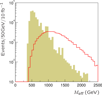
Figure 1: $M_{\rm eff}$ distribution for a typical mSUGRA point and SM backgrounds after cuts.

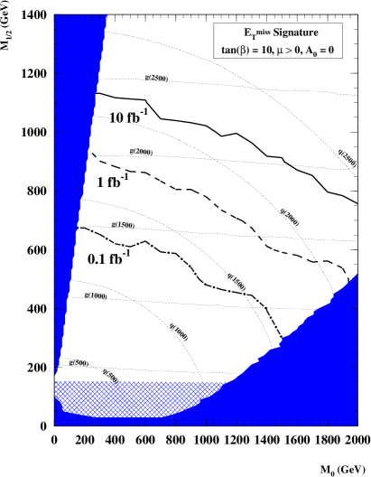
Figure 2: Search limits for the mSUGRA model in various channels for $10\,{\rm fb^{-1}}$ (left) and overall for various luminosities (right).[7]

2 Search for SUSY Particles at LHC

For masses in the TeV range SUSY production at the LHC is dominated by ${\tilde{g}}$ and ${\tilde{q}}$. Leptonic decays may or may not be large, but jets and $\hbox to0.0pt{\hbox to7.95831pt{\hfil/\hfil}\hss}E_{T}$ are always produced, and these generally give the best reach. Consider an mSUGRA with $m_{0}=100\,{\rm GeV}$, ${m_{1/2}}=300\,{\rm GeV}$, $A_{0}=0$, $\tan\beta=10$, $\mathop{\rm sgn}\mu=+$. Require $\hbox to0.0pt{\hbox to7.95831pt{\hfil/\hfil}\hss}E_{T}>100\,{\rm GeV}$, at least four jets with $E_{T}>100,50,50,50\,{\rm GeV}$, and plot as a measure of the hardness of the collision $M_{\rm eff}=\hbox to0.0pt{\hbox to7.95831pt{\hfil/\hfil}\hss}E_{T}+\sum_{j}E_{T,j}$. Then as Figure 1 shows the SUSY signal dominates for large $M_{\rm eff}$. The search limits from this sort of analysis for mSUGRA requiring $S>10$ and $S/\sqrt{B}>5$ reach more than $1\,{\rm TeV}$ for only $0.1\,{\rm fb^{-1}}$ and $2\,{\rm TeV}$ for $10\,{\rm fb^{-1}}$; see Figure 2.

While the AMSB model[8] is quite different, the reach in $M_{\tilde{g}},M_{\tilde{q}}$ is similar: above $2\,{\rm TeV}$ for $100\,{\rm fb^{-1}}$. Overall reach depends mainly on $\sigma(M_{\tilde{g}},M_{\tilde{q}})$ provided that $M_{\tilde{\chi}_{1}^{0}}\ll M_{\tilde{g}},M_{\tilde{q}}$, so one expects similar reach in most $R$-conserving models. This should be sufficient if SUSY is related to the naturalness of the electroweak scale.

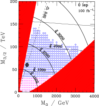
Figure 3: Search limits for the AMSB model.[9]

3 SUSY Particle Measurements

If $R$ parity is conserved, all SUSY particles decay to an invisible LSP ${\tilde{\chi}_{1}^{0}}$, so there are no mass peaks. But it is possible to identify particular decays and to measure their kinematic endpoints, determining combinations of masses.[10, 2] The three-body decay ${\tilde{\chi}}_{2}^{0}\to{\tilde{\chi}_{1}^{0}}\ell^{+}\ell^{-}$ gives a dilepton endpoint at $M_{\ell\ell}=M_{{\tilde{\chi}}_{2}^{0}}-M_{{\tilde{\chi}_{1}^{0}}}$, while ${\tilde{\chi}}_{2}^{0}\to{\tilde{\ell}}^{\pm}\ell^{\mp}\to{\tilde{\chi}_{1}^{0}}\ell^{+}\ell^{-}$ gives a triangular distribution with an endpoint at

$$M_{\ell\ell}=\sqrt{(M_{{\tilde{\chi}}_{2}^{0}}^{2}-M_{{\tilde{\ell}}}^{2})(M_{{\tilde{\ell}}}^{2}-M_{\tilde{\chi}_{1}^{0}}^{2})}/M_{\tilde{\ell}}\,.$$

These endpoints can be measured by requiring two isolated leptons in addition to multijet and $\hbox to0.0pt{\hbox to7.95831pt{\hfil/\hfil}\hss}E_{T}$ cuts like those described above. If lepton flavors are separately conserved, then contributions from two independent decays cancel in the combination $e^{+}e^{-}+\mu^{+}\mu^{-}-e^{\pm}\mu^{\mp}$ after acceptance corrections. The resulting distributions after cuts, Figure 4, are very clean and allow a precise measurement of the endpoint. The shape allows one to distinguish two-body and three-body decays.

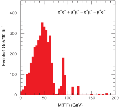
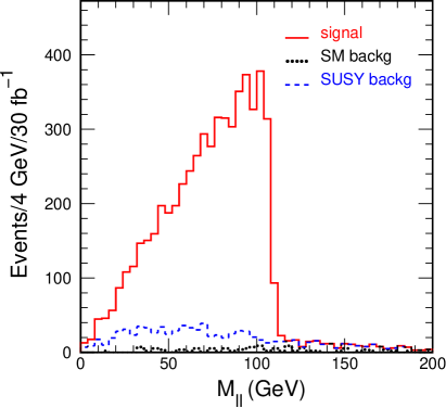
Figure 4: Examples of $M_{\ell\ell}$ for SUGRA points with ${\tilde{\chi}}_{2}^{0}\to{\tilde{\chi}_{1}^{0}}\ell^{+}\ell^{-},{\tilde{\chi}_{1}^{0}}Z$ (left) and for ${\tilde{\chi}}_{2}^{0}\to{\tilde{\ell}}_{R}^{\pm}\ell^{\mp}$ (right).[2]

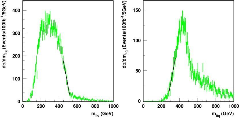
Figure 5: Distributions of the smaller $M(\ell\ell j)$ (left) and the larger $M(\ell\ell j)$ for $M_{\ell\ell}>M_{\ell\ell}^{\rm max}/\sqrt{2}$ (right) mSUGRA “Point 5.”[11]

Long decay chains allow more endpoint measurements. The dominant source of ${\tilde{\chi}}_{2}^{0}$ at mSUGRA “Point 5”[2] and similar points is ${\tilde{q}}_{L}\to{\tilde{\chi}}_{2}^{0}q\to{\tilde{\ell}}_{R}^{\pm}\ell^{\mp}q\to{\tilde{\chi}_{1}^{0}}\ell^{+}\ell^{-}q$. Assume the two hardest jets in the event are those from the squarks and for each calculate $M(\ell\ell j)$, $M^{<}(\ell j)$, and $M^{>}(\ell j)$. Then the smaller of each of these should be less than the endpoint $M_{\ell\ell q}$, $M_{\ell q}^{(>)}$, $M_{\ell q}^{(<)}$ for squark decay, while the larger $M(\ell\ell j)$ should be greater than the threshold $T_{\ell\ell q}$ requiring $M_{\ell\ell}>M_{\ell\ell}^{\rm max}/\sqrt{2}$. These endpoints are smeared by jet reconstruction, hadronic resolution, and mis-assignment of the jets that come from squark decays. Nevertheless, the distributions show clear structure at about the right positions.

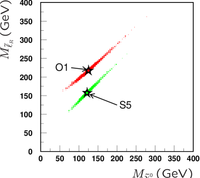
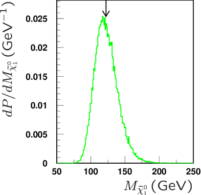
Figure 6: left: Scatter plot of $M_{{\tilde{\ell}}_{R}}$ vs. $M_{{\tilde{\chi}_{1}^{0}}}$ for two models consistent with measurements described in the text. Right: Projection of $M_{{\tilde{\chi}_{1}^{0}}}$.[11]

After accumulating high statistics and careful study, it should be possible to measure the endpoints to the expected hadronic scale accuracy, $\sim 1\%$. The $\ell\ell q$ threshold is more sensitive to hard gluon radiation, so it is assigned a larger error, $\sim 2\%$. Some distributions of the resulting masses derived assuming these errors are shown in Figure 6 for two models, mSUGRA Point 5 (S5) and an Optimized String Model (O1) with similar similar masses. Relations among the masses are determined to $\sim 1\%$ and are clearly sufficient to distinguish these models. The LSP mass is determined to $\sim 10\%$ by this analysis; since it is determined only by its effect on the kinematics of the decay, the fractional error on $M_{\tilde{\chi}_{1}^{0}}$ clearly diverges as $M_{\tilde{\chi}_{1}^{0}}^{2}/M_{\tilde{q}}^{2}\to 0$.

4 $h\to b\bar{b}$ Signatures

If ${\tilde{\chi}}_{2}^{0}\to{\tilde{\chi}_{1}^{0}}h$ is allowed, it may dominate over ${\tilde{\chi}}_{2}^{0}\to{\tilde{\chi}_{1}^{0}}\ell\ell$. This signal can be reconstructed using two $b$ jets measured in the calorimeter and tagged as $b$’s with the vertex detector. A typical signal using the expected $b$-tagging efficiency and light-quark rejection and the reach for such signals are shown in Figure 7. Such a Higgs signal in SUSY events might well be observed with less luminosity than $h\to\gamma\gamma$ or $h\to ZZ^{*}$ and so be the discovery channel for the light Higgs.

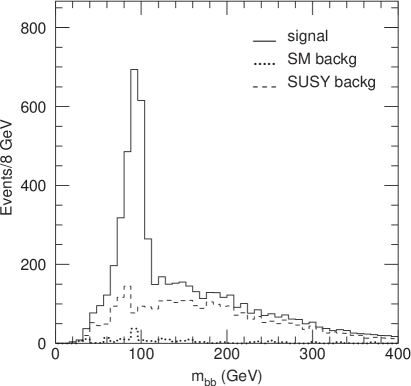
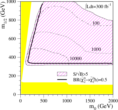
Figure 7: Left: Typical signal for $h\to b\bar{b}$ in SUSY event sample (“Point 5”). Right: Reach for this signal in mSUGRA.[2]

If a signal for $h\to b\bar{b}$ is observed in SUSY events, the $h$ can be combined with the two hardest jets in the event to measure the ${\tilde{q}}\to{\tilde{\chi}_{1}^{0}}hq$ endpoint in a way similar to the measurement of the $\ell\ell q$ endpoint. The resulting distribution is shown in Figure 8; the endpoint is consistent with what is expected. While the errors are worse than for the $\ell\ell q$ endpoint, the measurement is still useful.

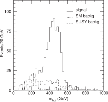
Figure 8: $M_{hj}$ distribution for events with $h\to b\bar{b}$.[2]

5 Heavy Gaugino Signatures

In mSUGRA and other typical SUSY models, the light charginos and neutralinos are mainly gaugino and so dominate the cascade decays, so that

$$B({\tilde{q}}_{L}\to{\tilde{\chi}}_{2}^{0}q)\sim 1/3,\quad B({\tilde{q}}_{L}\to{\tilde{\chi}}_{1}^{\pm}q^{\prime})\sim 2/3,\quad B({\tilde{q}}_{R}\to{\tilde{\chi}}_{1}^{0}q)\sim 1\,.$$

But even in the simplest mSUGRA model, ${\tilde{\chi}}_{4}^{0}$ and ${\tilde{\chi}}_{2}^{\pm}$ have a significant admixture of gaugino and so contribute in light-quark decays of squarks and gluinos.

Four ${\tilde{\chi}}_{4}^{0}/{\tilde{\chi}}_{2}^{\pm}$ decay chains can give OS, SF dileptons: ${\tilde{q}}_{L}\to{\tilde{\chi}}^{0}_{4}q\to{\tilde{\ell}}_{R}^{\pm}\ell^{\mp}q\to\tilde{\chi}^{0}_{2}\ell^{+}\ell^{-}q$ [D1]; ${\tilde{q}}_{L}{\tilde{\chi}}^{0}_{4}q\to{\tilde{\ell}}_{L}^{\pm}\ell^{\mp}q\to{\tilde{\chi}_{1}^{0}}\ell^{+}\ell^{-}q$ [D2]; ${\tilde{q}}_{L}{\tilde{\chi}}^{0}_{4}q\to{\tilde{\ell}}_{L}^{\pm}\ell^{\mp}q\to{\tilde{\chi}}_{2}^{0}\ell^{+}\ell^{-}q$ [D3]; and ${\tilde{q}}_{L}\to{\tilde{\chi}}_{2}^{\pm}q^{\prime}\to{\tilde{\nu}}_{\ell}\ell^{\pm}q^{\prime}\to{\tilde{\chi}}^{\pm}_{1}\ell^{\mp}q^{\prime}$ [D4]. In principle these four decay chains give four distinct $\ell^{+}\ell^{-}$ endpoints, but it seems impossible to resolve these even with $100\,{\rm fb^{-1}}$ of integrated luminosity. Nevertheless, there are $>10^{3}$ $\ell^{+}\ell^{-}$ events from heavy gauginos over substantial range of mSUGRA parameters; ${\tilde{\chi}}_{4}^{0}$ decays dominate for low $m_{0}$, while ${\tilde{\chi}}_{2}^{\pm}$ dominates for the region $m_{0}\sim{m_{1/2}}$.

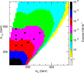
Figure 9: Event rates for heavy gaugino decays in mSUGRA. The dots show the 10 points studied in this analysis.[12]

Figure 10: $M_{\ell\ell}$ distributions for heavy chargino and neutralino decays at $m_{0},{m_{1/2}}=100,250\,{\rm GeV}$ (left) and $150,250\,{\rm GeV}$ right.[12]

Figure 11: Reach in mSUGRA for heavy gaugino signals.[12]

Event samples were generated and simulated for each of the ten points indicated in Figure 9. Events were required to have an $\ell^{+}\ell^{-}$ dilepton pair, $M_{\ell\ell}>100\,{\rm GeV}$, $\hbox to0.0pt{\hbox to7.95831pt{\hfil/\hfil}\hss}E_{T}>100\,{\rm GeV}$, $\geq 4$ jets, and $M_{\rm eff}>600\,{\rm GeV}$. To suppress SM backgrounds a cut $M_{T2}>80\,{\rm GeV}$ was also made, where[13]

$$M_{T2}^{2}\equiv\min_{\hbox to0.0pt{\hbox to3.52188pt{\hfil/\hfil}\hss}p_{1}+\hbox to0.0pt{\hbox to3.52188pt{\hfil/\hfil}\hss}p_{2}=\hbox to0.0pt{\hbox to3.52188pt{\hfil/\hfil}\hss}p_{T}}\left[\max{\left\{m_{T}(p_{T,\ell_{1}},\hbox to0.0pt{\hbox to5.03125pt{\hfil/\hfil}\hss}p_{1}),m_{T}(p_{T,\ell_{2}},\hbox to0.0pt{\hbox to5.03125pt{\hfil/\hfil}\hss}p_{2})\right\}}\right]$$

is the minimum transverse mass obtained by partitioning the observed $\hbox to0.0pt{\hbox to7.95831pt{\hfil/\hfil}\hss}E_{T}$ between two massless particles. Note that $M_{T2}<M_{W}$ for $t$ and $W$ backgrounds.

Results for $m_{0},{m_{1/2}}=100,250\,{\rm GeV}$ and $150,250\,{\rm GeV}$ are shown in Figure 10. Evidently the signal is observable over the SUSY and SM background in both cases. The estimated statistical error on the endpoint is about $\pm 4\,{\rm GeV}$ in both cases. The $5\sigma$ reach for such signals in mSUGRA is indicated by the dark curve in Figure 11. Heavy gaugino signals are rather model dependent, so the ability to study them is important for understanding the SUSY model.

6 Third-Generation Squark Signatures

The properties of the third-generation squarks $\tilde{b}_{1,2}$ and $\tilde{t}_{1,2}$ are important for understanding the SUSY model, but their signatures are typically complex. The main production mechanism is ${\tilde{g}}$ production and decay. Consider for mSUGRA with $m_{0}=100\,{\rm GeV}$, ${m_{1/2}}=300\,{\rm GeV}$, $A_{0}=-300\,{\rm GeV}$, $\tan\beta=10$, $\mathop{\rm sgn}\mu=+$ the processes

$${\tilde{g}}\to t\tilde{t}_{1}^{*}\to t\bar{b}{\tilde{\chi}}_{1}^{-},\qquad{\tilde{g}}\to\bar{b}\tilde{t}_{1}\to t\bar{b}{\tilde{\chi}}_{1}^{-}$$

Then the $M(t\bar{b})$ endpoint can be used to measure a combination of masses of the squark masses.

The analysis[14] requires as usual multiple hard jets and large $\hbox to0.0pt{\hbox to7.95831pt{\hfil/\hfil}\hss}E_{T}$ plus two jets tagged as $b$’s and two other jets $j$ not tagged as $b$’s and consistent with $t\bar{b}\to jjb\bar{b}$. The resulting $M_{t\bar{b}}$ distribution is still dominated by combinatorial background. The next step is to select sidebands around $M_{jj}=M_{W}$, rescale the jet momenta to $M_{W}$, and subtract to determine $t\bar{b}$ signal. The $M(t\bar{b})$ mass distributions for one point before and after subtraction are shown in Figure 12. The fitted endpoint for this case is $443.2\pm 7.4\,{\rm GeV}$ compared to expected $459\,{\rm GeV}$. A similar agreement between reconstructed and expected endpoints was found for all twelve points studied. Heavy squark signatures are clearly difficult, but it appears possible to use a sideband analysis such as this to study them with the ATLAS detector.

Figure 12: Reconstructed $M_{tb}$ distribution before sideband subtraction (left) and after subtraction (right).[14]

7 $\tau$ Signatures

The mSUGRA model assumes $\tilde{e}$-$\tilde{\mu}$ universality, and this is certainly suggested by the stringent limits on $\mu\to e\gamma$. Even in the simplest mSUGRA model, however, the ${\tilde{\tau}}$ behave differently than $\tilde{e}$ and $\tilde{\mu}$ because of Yukawa contributions to the RGE’s, gaugino-Higgino mixing, and ${\tilde{\tau}}_{L}$-${\tilde{\tau}}_{R}$ mixing, which is $\propto m_{\tau}$. Hence $\tau$’s provide unique information and might even be dominant in SUSY decays.

Figure 13: $\tau$ identification in ATLAS.[2]

The ATLAS (and CMS) vertex detectors cannot cleanly identify $\tau\to\ell\nu\bar{\nu}$, so it is necessary to rely on hadronic $\tau$ decays. The background for such decays is much larger than that for electrons and muons. The $\tau$ efficiency vs. jet rejection shown in Figure 13 should be compared with the $>10^{4}$ rejection for 90% efficiency expected for electrons and muons. Furthermore, all $\tau$ decays contain missing neutrinos. For $H,A\to\tau\tau$ one can project $\hbox to0.0pt{\hbox to7.95831pt{\hfil/\hfil}\hss}E_{T}$ on the measured $\tau$ directions to reconstruct the $\tau\tau$ mass, but this is not possible for SUSY because of the dominant $\hbox to0.0pt{\hbox to7.95831pt{\hfil/\hfil}\hss}E_{T}$ from the ${\tilde{\chi}_{1}^{0}}$’s.

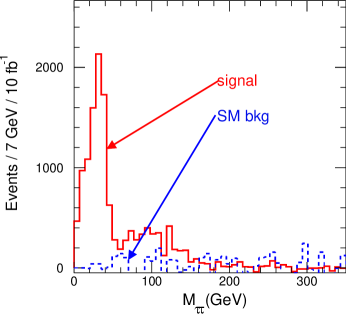
Figure 14: Reconstructed visible $\tau\tau$ mass in a mSUGRA event sample.[2]

Decays into $\tau$’s are generally enhanced for $\tan\beta\gg 1$. A mSUGRA model with $m_{0}={m_{1/2}}=200\,{\rm GeV}$, $A_{0}=0$, $\tan\beta=45$ gives ${\tilde{\chi}}_{2}^{0}\to{\tilde{\tau}}_{1}\tau$ and ${\tilde{\chi}}_{1}^{\pm}\to{\tilde{\tau}}_{1}\nu_{\tau}$ with branching ratios close to unity. For events from this point, a simple model for the detector response turns a sharp edge at $M_{\tau\tau}=59.64\,{\rm GeV}$ into the distribution shown in Figure 14. The visible momentum or mass depends both on the momentum and on the polarization of the $\tau$. Measuring the $\tau$ polarization requires separating different $\tau$ decay modes; the visible energy depends strongly on polarization for $\tau\to\pi\nu$ but weakly for $\tau\to a_{1}\nu$. Such a separation of decay appears to be possible, albeit difficult: for example $\tau\to\pi\nu$ has a single track with $p=E$ and low electromagnetic energy. Recent work based on full GEANT simulation has given an encouraging indication that the $\tau\tau$ endpoint can be inferred from the visible $\tau\tau$ mass.

8 GMSB Signatures

While the mSUGRA model remains after 20 years perhaps the most attractive paradigm for SUSY breaking, it may not be correct. In the GMSB model SUSY breaking is communicated via gauge interactions at a scale much less than the Planck scale, so the gravitino ${\tilde{G}}$ is very light. GMSB phenomenology[15] depends on the nature and lifetime of NLSP (${\tilde{\chi}_{1}^{0}}$ or ${\tilde{\ell}}$) to decay into the ${\tilde{G}}$. In general the GMSB model produces longer decay chains with more precisely measured decay products,[2] so reconstructing masses is considerably easier than in mSUGRA.

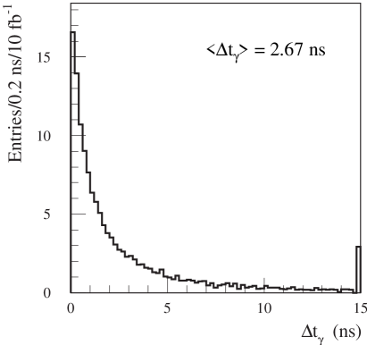
Figure 15: Angular (left) and time (right) distributions for photons from ${\tilde{\chi}_{1}^{0}}\to{\tilde{G}}\gamma$ in ATLAS.[2]

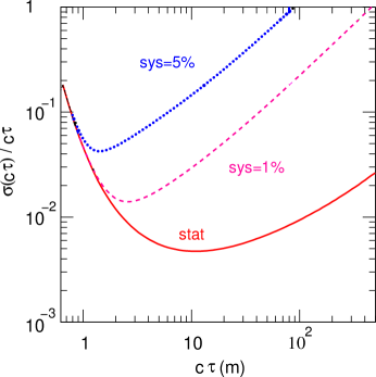
Figure 16: Error on slepton lifetime for various assumptions on the systematic error on the acceptance.[16]

The GMSB model can give a number of special signatures related to NLSP decay. If the NLSP is a ${\tilde{\chi}_{1}^{0}}$, its lifetime for ${\tilde{\chi}_{1}^{0}}\to{\tilde{G}}\gamma$ can range from very short to very long. Short lifetimes can be detected by using the Dalitz decays ${\tilde{\chi}_{1}^{0}}\to{\tilde{G}}\ell^{+}ell^{-}$ with branching ratios of a few percent. Long lifetimes can be detected by looking for (rare) non-pointing photons in SUSY events. The ATLAS electromagnetic calorimeter has both good angular resolution in the polar angle, $\Delta\theta\approx{60\,{\rm mr}\over\sqrt{E/1\,{\rm GeV}}}$, and good timing resolution, $\Delta t\approx 100\,{\rm ps}$. Both can be used to detect non-prompt photons from long-lived particles like ${\tilde{\chi}_{1}^{0}}$ produced with $\beta<1$. Such signals give a sensitivity up to $c\tau\sim 100\,{\rm km}$, much greater than what is expected in the GMSB model.

For other choices of the parameters the GMSB model might give long-lived sleptons, which look like muons with $\beta<1$ in a detector. The ATLAS muons chambers give a time-of-flight resolution in the $1\,{\rm ns}$ range over a distance of about $10\,{\rm m}$, making it possible to reconstruct both the momentum and the mass of the slepton. The slepton lifetime can be determined by comparing the rates for events with one and two reconstructed sleptons as shown in Figure 16. The statistical error is small; the dominant systematic error is difficult to estimate without real data. Another approach would be to look for sleptons decaying into non-pointing tracks in the central detector. This should be more sensitive for long lifetimes, but estimating the sensitivity requires studying the pattern recognition for such non-pointing tracks.

9 Full Simulation of SUSY Events

Most studies of SUSY signatures in ATLAS have been based on fast simulation such as ATLFAST. While this should represent the ultimate performance of the detector, it does not necessarily represent the effort needed to achieve that performance. Therefore, a sample of 100k SUSY events has recently been simulated with full GEANT for an mSUGRA point with

$$m_{0}=100\,{\rm GeV},\ {m_{1/2}}=300\,{\rm GeV},\ A_{0}=-300\,{\rm GeV},\ \tan\beta=6,\ \mathop{\rm sgn}\mu=+$$

The simulation of each event takes about $10^{3}\,{\rm s}$, compared with about $1\,{\rm s}$ for event generation and fast simulation. Thus, such a study represents a large effort.

Most of the effort so far has been devoted to debugging the reconstruction software, so the results are not yet useful for assessing the performance of the ATLAS detector for SUSY. However, a few physics plots have been produced using cuts based on previous fast simulation studies like those described above. As an example, Figure 17 shows the $e^{+}e^{-}+\mu^{+}\mu^{-}-e^{\pm}\mu^{\mp}$ mass distribution from full simulation of SUSY events after corrections for the average $e$ and $\mu$ acceptance and for the $e$ energy scale. It is encouraging that the distribution is quite similar to that obtained from fast simulation.

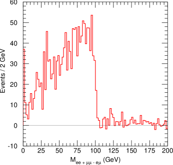
Figure 17: $e^{+}e^{-}+\mu^{+}\mu^{-}-e^{\pm}\mu^{\mp}$ mass distribution from full GEANT simulation after corrections for average acceptance and electron energy scale.[17]

10 Higgs Signatures

SUSY requires Higgs bosons. In the Minimal Supersymmetric Standard Model (MSSM) there are two Higgs doubles and hence after electroweak symmetry breaking five Higgs bosons, $h$, $H$, $A$, and $H^{\pm}$. The light, $CP$-even, $h$ satisfies $M_{h}<M_{Z}$ at tree level $M_{h}\mathrel{\hbox to0.0pt{\raise 2.20013pt\hbox{$<$}\hss}{\lower 2.20013pt\hbox{$\sim$}}}130\,{\rm GeV}$ after loop corrections. In many although not all SUSY models the $h$ is very similar to a SM Higgs of the same mass.

The search for SM-like Higgs bosons has been a principle design goal of both ATLAS and CMS, and a large amount of effort has been devoted to studies of how to search for such particles. The global summary of these studies is shown in Figure 18: for each SM Higgs mass there is at least one channel giving a significance of more than $5\sigma$ for an integrated luminosity of $100\,{\rm fb^{-1}}$, and the combined significance of all channels is greater than about $10\sigma$.

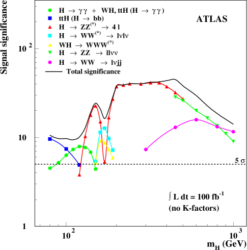
Figure 18: Significance of SM Higgs modes in ATLAS for $100\,{\rm fb^{-1}}$.[2]

Recently, more effort has been devoted to studies of how to measure the properties of Higgs bosons once they are discovered. The key for doing this is to observe the Higgs boson in more than one production and/or decay channel.[18] While $gg\to h$ is the dominant production process at the LHC, $WW\to h$ is also significant and plays a crucial role in the analysis. These events can be identified by requiring hard forward jets resulting from the radiation of the $W$’s from incoming quarks, $q\to Wq^{\prime}$, and no additional central jets.

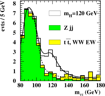
Figure 19: Reconstructed $M_{\tau\tau}$ distribution from $WW\to h\to\tau\tau$ after cuts.[19]

A typical result from such a study is shown in Figure 19. Events were selected using a combination of $e\mu$, $ee+\mu\mu$, and $\ell h$ modes requiring a double forward jet tag and a central jet veto; $M_{\tau\tau}$ was reconstructed by projecting $\hbox to0.0pt{\hbox to7.95831pt{\hfil/\hfil}\hss}E_{T}$ on the measured $\tau$ directions. The accepted cross section is about $1.0\,{\rm fb}$ on a total SM background of $0.5\,{\rm fb}$. Thus this channel can be used to measure the product of $\Gamma_{h,WW}$ and $\Gamma_{h,\tau\tau}$. Combining a number of such measurements can give a good determination of the properties of the $h$, although a linear collider with sufficient energy and luminosity could do better.

Figure 20: Transverse mass distribution for $gb\to tH^{-}$ with $t\to q\bar{q}b$ and $H^{-}\to\tau^{-}\bar{\nu}$.[20]

It may also be possible to reconstruct heavy Higgs bosons, especially for $\tan\beta\gg 1$. An example of the reconstruction of $gb\to H^{-}t$ with $H^{-}\to\tau^{-}\nu$ is shown in Figure 20. Since the signature is a narrow hadronic $\tau$ plus reconstructed $t$, events were selected requiring an identified hadronic $\tau$ jet plus two non-$b$ jets and a $b$ jet consistent with $t$ kinematics. This analysis relies on the fact that in $H^{-}\to\tau_{R}\nu\to\pi^{-}\nu\nu$ the $\pi^{-}$ is hard and so is well separated from SM backgrounds.

11 Outlook

If SUSY exists at the TeV mass scale, ATLAS should find signatures for it quite easily at the LHC. If $R$ parity is conserved, no mass peaks for SUSY particles can be reconstructed, but several techniques have been developed to measure combinations of SUSY masses using kinematic distributions of observable decay products.

While the details of SUSY analyses at the LHC certainly depend on the details of the SUSY model, it is possible to sketch a general outline of how ATLAS could proceed first to search for and then to study SUSY with $R$-parity conservation:

1. Search for an excess of multijet + $\hbox to0.0pt{\hbox to7.95831pt{\hfil/\hfil}\hss}E_{T}$ events over the SM expectation, and observe the $M_{\rm eff}$ at which this emerges from the background.

2. If such an excess is found, select a SUSY-dominated sample using simple kinematic cuts.

3. Look in this sample for special features such as prompt $\gamma$’s or long-lived ${\tilde{\ell}}$; either of these may occur in GMSB.

4. Look in the SUSY-dominated sample for $\ell^{\pm}$, $\ell^{+}\ell^{-}$, $\ell^{\pm}\ell^{\pm}$, $b$ jets, hadronic $\tau$’s, etc.

5. Try simple endpoint-type analyses.

Carrying out such an initial study seems quite feasible. Its results would of course guide further more detailed and more model dependent analyses.

I thank my many ATLAS collaborators who have contributed to the work presented here. This work was supported in part by the United States Department of Energy under Contract DE-AC02-98CH10886.

References

- [1] A.H. Chamseddine, R. Arnowitt, and P. Nath Phys. Rev. Lett. 49, 970 (1982).
- [2] ATLAS Collaboration, ATLAS Detector and Physics Performance Technical Design Report, CERN/LHCC/99-14 (1999).
- [3] G. Corcella, et al., hep-ph/0210213.
- [4] H. Baer, et al., hep-ph/0001086.
- [5] T. Sjostrand, et al., hep-ph/0010017
- [6] http://wwwasdoc.web.cern.ch/wwwasdoc/geant/geantall.html
- [7] D. Tovey, Eur. Phys. J. bf C4, N4 (2002)
- [8] L. Randall and R. Sundrum, hep-th/9810155, Nucl. Phys. B557, 79 (1999); G.F. Giddice, M.A. Luty, H. Murayama, and R. Rattazzi, hep-ph/9810422, JHEP 12, 27 (1998),
- [9] A.J. Barr, et al., hep-ph/0208214, JHEP 0303, 045 (2003).
- [10] I. Hinchliffe, et al., hep-ph/9610544, Phys. Rev. D55, 5520 (1997).
- [11] B.C. Allanach, et al., hep-ph/0007009, JHEP 0009, 004 (2000).
-
[12]
G. Polesello,
http://agenda.cern.ch/askArchive.php?base=agenda&categ=a03395&id=a03395s0t4/transparencies. - [13] A. Barr, et al., hep-ph/0304226.
- [14] J. Hisano, et al., hep-ph/0304214.
- [15] S. Ambrosanio, et al., hep-ph/9605398, Phys. Rev. D54, 5395 (1996). For a review see G.F. Giudice and R. Rattazzi, hep-ph/9801271, Phys. Rept. 322, 419 (1999).
- [16] S. Ambrosanio, et al., hep-ph/0010081, JHEP 0101 014 (2001).
-
[17]
http://agenda.cern.ch/askArchive.php?base=agenda&categ=a031081&id=a031081s10t4/transparencies. - [18] D. Rainwater and D. Zeppenfeld, hep-ph/9712271, JHEP 9712, 005 (1997); D. Zeppenfeld, et al., hep-ph/0002036, Phys. Rev. D62, 013009 (2000).
-
[19]
S. Asai, et al.,
http://cdsweb.cern.ch/search.py?recid=8912. - [20] K. Assamagan, et al., hep-ph/0203121, Eur. Phys. J. direct C4, 9 (2002).