Higgs-Boson Mass Limits and Precise Measurements
beyond the Standard Model

Abstract

The triviality and vacuum stability bounds on the Higgs-boson mass ($m_{h}$) were revisited in presence of weakly-coupled new interactions parameterized in a model-independent way by effective operators of dimension 6. The constraints from precision tests of the Standard Model were taken into account. It was shown that for the scale of new physics in the region $\Lambda\simeq 2\div 50\;\hbox{TeV}$ the Standard Model triviality upper bound remains unmodified whereas it is natural to expect that the lower bound derived from the requirement of vacuum stability is substantially modified depending on the scale $\Lambda$ and strength of coefficients of effective operators. A natural generalization of the standard triviality condition leads also to a substantial reduction of the allowed region in the ($\Lambda,m_{h}$) space.

I Introduction

In spite of a huge experimental effort, the Higgs particle, the last missing ingredient of the Standard Model (SM) of electroweak interactions has not been yet discovered. For a Higgs-boson mass $\lower 2.15277pt\hbox{$\>\buildrel<\over{\sim}\>$}115\;\hbox{GeV}$ the most promising production channel at LEP2 is through radiation off a $Z$-boson: $e^{+}e^{-}\to Zh$; using this reaction the LEP experiments obtained the limit higgs_limit $m_{h}>113.2\;\hbox{GeV}$ on the SM Higgs-boson mass. The Higgs particle also contributes radiatively to several well measured quantities, which has been used to derive the complementary upper bound prec_data $m_{h}\lower 2.15277pt\hbox{$\>\buildrel<\over{\sim}\>$}212\;\hbox{GeV}$ at 95 % C.L.. The data then leave a rather narrow range for $m_{h}$, however it must be emphasized that these constraints are highly model-dependent and are significantly weakened in most extensions of the SM .

There also exist theoretical, restrictions of $m_{h}$ based on the so-called triviality and vacuum stability arguments. As it is well know triviality the renormalized $\phi^{4}$ theory cannot contain an interaction term ($\lambda\phi^{4}$) for any non-zero scalar mass: the theory must be trivial. Within a perturbative approach the statement corresponds to the fact that for any non-zero scalar mass  there exists a finite energy scale at which $\lambda$ diverges (the Landau pole). Consequently this theory is consistent for all energy scales only when it describes non-interacting scalars. An analogous effect occurs in the scalar sector of the SM, though modified to some extent by presence of gauge and Yukawa interactions. This, however, does not necessarily imply a trivial scalar sector, since we do not demand the validity of the SM at arbitrarily high energy scales. For example, it is often assumed that the SM represents the low energy limit of some underlying more fundamental theory whose heavy excitations decouple at low energy, but become manifest at a scale $\Lambda$. Within this scenario the SM is an effective theory containing the dominant terms in a $1/\Lambda$ expansion; any process occurring at a typical energy $E$ will then receive corrections suppressed by powers of $E/\Lambda$ generated by the sub-leading interactions.

If the SM is to be accurate for energies below $\Lambda$ the Landau pole should occur at scale $\Lambda$ or above, and this condition gives a ($\Lambda$-dependent) upper bound on $m_{h}$ triv_bounds . On the other hand, for sufficiently small $m_{h}$ radiative corrections can destabilize the ground state. This occurs if the running scalar self-coupling constant $\lambda$ becomes negative at some scale, that can be again identified with the scale of new physics $\Lambda$. Alternatively requiring the SM vacuum to be stable for scales below $\Lambda$ implies a ($\Lambda$-dependent) lower bound on $m_{h}$ vacuum_bounds .

The consequences of the above arguments (triviality and vacuum stability) are usually discussed assuming pure SM interactions. However, if the scale of new physics is sufficiently low (of the order of a few TeV) one would expect for the sub-dominant effects to significantly influence both the renormalization group evolution and the scalar effective potential, and thus modify the corresponding bounds on the Higgs-boson mass.

It then becomes interesting to determine the manner in which heavy physics with scales in the $10\;\hbox{TeV}$ region can modify the stability and triviality bounds on the Higgs-boson mass. In this paper we address this question in a model-independent way by parameterizing the heavy physics effects using an effective Lagrangian satisfying the SM gauge symmetries. This issue was investigated in previous publications Grzadkowski:2001vb , but without taking into account the restrictions generated by the precision tests of the SM. The analysis presented here remedies this deficiency by including these constraints (to the one-loop approximation in the SM and at tree level in the effective dim 6 operators); for other works discussing vacuum stability including some effective operators see Refs. Datta:1996ni ; Casas:2000mn ; Burgess:2002tj .

The paper is organized as follows. In Sec. II, we define the Lagrangian relevant for our discussion. Sec. III presents the relevant renormalization group running equations including effects of non-standard interactions. In Sec. IV we calculate the effective potential with one insertion of an effective operator. Sec. V contains the methodology that we have applied and our numerical results. Concluding remarks are given in Sec. VI.

II Non-Standard Interactions

Our study of the stability and triviality constraints on the Higgs-boson mass will be based on the SM Lagrangian modified by the addition of a series of effective operators whose coefficients parameterize the low-energy effects of the heavy physics leff.refs . Assuming that these non-standard effects decouple implies decoupling that all physical effects disappear in the $\Lambda\to\infty$ limit and, in particular, that the effective operators of dimension $>4$ appear multiplied by appropriate inverse powers of $\Lambda$. Leading effects are then generated by operators of mass-dimension 6 (dimension 5 operators necessarily violate lepton number effe_oper and are presumably associated with new physics at very large scales since they lead to very small effects; accordingly they can be safely ignored hereafter). Given our emphasis on Higgs-boson physics the effects of all fermions excepting the top-quark can also be ignored . We then have

$${\cal L}_{\rm tree} = -\frac{1}{4}F_{\mu\nu}^{i}F^{i\mu\nu}-\frac{1}{4}B_{\mu\nu}B^{\mu\nu}+\left|D\phi\right|^{2}-\lambda\left(|\phi|^{2}-\frac{1}{2}v^{2}\right)^{2}+$$ (1)

$$i\bar{q}\not\!\!Dq+i\bar{t}\not\!\!Dt+f\left(\bar{q}\tilde{\phi}t+\hbox{h.c.}\right)+\sum_{i}\frac{\alpha_{i}}{\Lambda^{2}}{\cal O}_{i},$$

where $\phi$ ($\tilde{\phi}=-i\tau_{2}\phi^{*}$), $q$ and $t$ denote the scalar doublet, third generation left-handed quark doublet and the right-handed top singlet, respectively. $D$ represents a covariant derivative, and $F_{\mu\nu}^{i}$ and $B_{\mu\nu}$ the $SU(2)$, $U(1)$ field strengths whose corresponding gauge couplings we denote by $g$ and $g^{\prime}$. The factors $\alpha_{i}$ are unknown coefficients that parameterize the low-energy effects of the non-standard interactions and we have neglected contributions $\propto 1/\Lambda^{4}$.

For weakly coupled theories, the $\alpha_{i}$ that can be generated only through loop effects are sub-dominant as they are suppressed by numerical factors $\sim 1/(4\pi)^{2}$ tree_oper ; hence we will consider only those operators that can be generated at tree-level by the heavy physics. Even with all the above restrictions there remain 16 operators that involve exclusively the fields in (1). Of these only 5 contribute directly to the effective potential, the remaining 11 would affect our results only through their RG mixing which, being suppressed by a factor $\sim G_{F}\Lambda^{2}$ (where $G_{F}$ denotes the Fermi constant) are expected to play a sub-dominant role. In the calculations below we will include only one of these operators for illustration purposes; our results justify the claim that the corresponding effects are small.

Specifically we include the following set of operators:

$$\begin{array}[]{lll}{{\cal O}_{\phi}}=\frac{1}{3}|\phi|^{6}&{{\cal O}_{\partial\phi}}=\frac{1}{2}\left(\partial|\phi|^{2}\right)^{2}&{{\cal O}_{\phi}^{(1)}}=|\phi|^{2}\left|D\phi\right|^{2}\cr{{\cal O}_{\phi}^{(3)}}=\left|\phi^{\dagger}D\phi\right|^{2}&{{\cal O}_{t\phi}}=|\phi|^{2}\left(\bar{q}\tilde{\phi}t+\hbox{h.c.}\right)&{{\cal O}_{qt}^{(1)}}=\frac{1}{2}\left|\bar{q}t\right|^{2}\end{array}$$ (2)

where ${{\cal O}_{\phi}}$, ${{\cal O}_{\partial\phi}}$, ${{\cal O}_{\phi}^{(1)}}$, ${{\cal O}_{\phi}^{(3)}}$, ${{\cal O}_{t\phi}}$ are the 5 operators contributing to the effective potential, while ${{\cal O}_{qt}^{(1)}}$ is included to estimate the effects of RG mixing.

Of the first five operators only ${{\cal O}_{\phi}}=\frac{1}{3}|\phi|^{6}$ contributes at the tree level to the scalar potential:

$$V^{(\rm tree)}=-\eta\Lambda^{2}|\phi|^{2}+\lambda|\phi|^{4}-{\alpha_{\phi}\over 3\Lambda^{2}}|\phi|^{6}$$ (3)

where we have used the notation: $\eta\equiv\lambda v^{2}/\Lambda^{2}$.

III The renormalization group equations

In order to test the high energy behavior of the scalar potential one has to derive the RG running equations for $\lambda$, $\eta$ and $\alpha_{\phi}$. The $\beta$ functions for these parameters are influenced by all the operators in (2) and by the gauge and Yukawa interactions, so the full RG evolution also require the $\beta$ function for the corresponding couplings. In the following calculations we will adopt dimensional regularization and $\overline{\rm MS}$ renormalization scheme. We will restrict ourselves to the one-loop approximation keeping all SM contributions as well as those linear in the effective operators (2).

Defining $\bar{\alpha}=\alpha_{\partial\phi}+2\alpha_{\phi}^{(1)}+\alpha_{\phi}^{(3)}$, the resulting evolution equations are:

$${d\lambda\over dt} = 12\lambda^{2}-3f^{4}+6\lambda f^{2}-{3\over 2}\lambda\left(3g^{2}+g^{\prime}{}^{2}\right)+{3\over 16}\left(g^{\prime}{}^{4}+2g^{2}g^{\prime}{}^{2}+3g^{4}\right)$$ (5)

$$+2\eta\left[2\alpha_{\phi}+\lambda\left(3\alpha_{\partial\phi}+4\bar{\alpha}+\alpha_{\phi}^{(3)}\right)\right]$$

$${d\eta\over dt} = 3\eta\left[2\lambda+f^{2}-{1\over 4}\left(3g^{2}+g^{\prime}{}^{2}\right)\right]+2\eta^{2}\bar{\alpha}$$ (6)

$${df\over dt} = {9\over 4}f^{3}-f\left(4g_{s}^{2}+{9\over 8}g^{2}+{17\over 24}g^{\prime}{}^{2}\right)-3\eta\alpha_{t\phi}+{f\eta\over 2}\left(\bar{\alpha}+3\alpha_{qt}^{(1)}\right)$$ (7)

$${d\alpha_{\phi}\over dt} = 9\alpha_{\phi}\left(6\lambda+f^{2}\right)+12\lambda^{2}(9\alpha_{\partial\phi}+6\alpha_{\phi}^{(1)}+5\alpha_{\phi}^{(3)})+36\alpha_{t\phi}f^{3}-{9\over 4}\left(3g^{2}+g^{\prime}{}^{2}\right)\alpha_{\phi}$$ (9)

$$-{9\over 8}\left[2\alpha_{\phi}^{(1)}g^{4}+\left(\alpha_{\phi}^{(1)}+\alpha_{\phi}^{(3)}\right)\left(g^{2}+g^{\prime}{}^{2}\right)^{2}\right]$$

$${d\alpha_{\partial\phi}\over dt} = 2\lambda\left(7\alpha_{\partial\phi}-\alpha_{\phi}^{(1)}+\alpha_{\phi}^{(3)}\right)+6f\left(f\alpha_{\partial\phi}-\alpha_{t\phi}\right)$$ (10)

$${d\alpha_{\phi}^{(1)}\over dt} = 2\lambda\left(\bar{\alpha}+3\alpha_{\phi}^{(1)}\right)+6f\left(f\alpha_{\phi}^{(1)}-\alpha_{t\phi}\right)$$ (11)

$${d\alpha_{\phi}^{(3)}\over dt} = 6(\lambda+f^{2})\alpha_{\phi}^{(3)}$$ (12)

$${d\alpha_{t\phi}\over dt} = -3f(f^{2}+\lambda)\alpha_{qt}^{(1)}+\left({15\over 4}f^{2}-12\lambda\right)\alpha_{t\phi}-{1\over 2}f^{3}\left(2\alpha_{\partial\phi}+\alpha_{\phi}^{(1)}+\alpha_{\phi}^{(3)}\right)$$ (13)

$${d\alpha_{qt}^{(1)}\over dt} = {3\over 2}\alpha_{qt}^{(1)}f^{2}$$ (14)

where $8\pi^{2}t\equiv\log(\kappa/m_{Z})$, $\kappa$ denotes the renormalization scale and $g_{s}$ is the QCD coupling constant. The RG equations for $g$, $g^{\prime}$, and $g_{s}$; $dg/dt=-19g^{3}/12$, $dg^{\prime}/dt=+41g^{\prime}{}^{3}/12$, and $dg_{s}/dt=-7/2g_{s}^{3}$ are not modified by the $\alpha_{i}$.

From this set of equations it is straightforward to obtain the traditional triviality constraints on $m_{h}$ as a function of $\Lambda$ by requiring that the position of the Landau pole in the evolution of $\lambda(t)$ lies beyond the scale $\Lambda$. At this point it is important to note that within perturbation theory the triviality constraint is not obtained from the requirement that the Higgs mass diverges at scale $\Lambda$, but form the condition that the theory remains perturbative at all scales below $\Lambda$. The triviality bound on $m_{h}$ will be obtained then by requiring $\lambda$ and $|\alpha_{i}|$ to remain below certain specified values (chosen so as to insure perturbative consistency) up to the scale $\Lambda$; the details are presented in Sect.V

In order to solve the equations (14) we have to specify appropriate boundary conditions. For the SM parameters these are determined by requiring that the correct physical parameters (such as the Higgs-boson mass, top-quark masses, etc.) are obtained at the electroweak scale, and that the correct SM ground state is realized; the details of the implementation of these low scale initial conditions are also described in Sect.V. In contrast, the boundary conditions for the $\alpha_{i}$ are naturally specified at the scale $\kappa=\Lambda$ since it is below this scale that (1) is expected to describe the effects of the heavy excitations; following Ref. tree_oper we will use the (natural) choices $\alpha_{i}|_{\kappa=\Lambda}=\pm 1$.

The triviality bound is obtained by solving the equations (14) with the mixed (defined partly at the electroweak scale $m_{Z}$ and partly at the new-physics scale $\Lambda$) boundary conditions described above and requiring that triviality constraints (see Sec.V) are saturated, and this provides a relationship between $m_{h}$ and $\Lambda$. For example, if we require only $\lambda(\kappa)<\pi/2$ for $m_{Z}\leq\kappa\leq\Lambda$, we obtain the plot in Fig.2; imposing also the additional conditions $|\alpha_{i}(\kappa)|<3/2$ yields a much richer structure discussed in Sec.V and illustrated by the plots in Fig.3.

IV The effective potential

In order to investigate the vacuum structure of the effective theory we first calculate the effective potential:

$$V_{\rm eff}=-\sum_{N}\frac{1}{N!}\Gamma^{(N)}(0)\bar{\varphi}^{n},$$ (15)

where $\Gamma^{(N)}(0)$ are N-point one-particle-irreducible Green‘s functions with zero external momenta and $\bar{\varphi}$ is the classical scalar field. Adopting the Landau gauge  we find:

$$V_{\rm eff}(\bar{\varphi}) = -\eta\Lambda^{2}|\bar{\varphi}|^{2}+\lambda|\bar{\varphi}|^{4}-{\alpha_{\phi}|\bar{\varphi}|^{6}\over 3\Lambda^{2}}$$

$$+{1\over 64\pi^{2}}\Biggl{[}H^{2}\left(\ln{H\over\kappa^{2}}-{3\over 2}\right)+3G^{2}\left(\ln{G\over\kappa^{2}}-{3\over 2}\right)+6W^{2}\left(\ln{W\over\kappa^{2}}-{5\over 6}\right)$$

$$+3Z^{2}\left(\ln{Z\over\kappa^{2}}-{5\over 6}\right)-12T^{2}\left(\ln{T\over\kappa^{2}}-{3\over 2}\right)-4\eta^{2}\Lambda^{4}\left(\ln{\eta\Lambda^{2}\over\kappa^{2}}-{3\over 2}\right)\Biggr{]},$$

for

$$H = (6\lambda|\bar{\varphi}|^{2}-\eta\Lambda^{2})-\left[(6\lambda|\bar{\varphi}|^{2}-\eta\Lambda^{2})(2\alpha_{\partial\phi}+\alpha_{\phi}^{(1)}+\alpha_{\phi}^{(3)})+5\alpha_{\phi}|\bar{\varphi}|^{2}\right]{|\bar{\varphi}|^{2}\over\Lambda^{2}}$$ (18)

$$G = (2\lambda|\bar{\varphi}|^{2}-\eta\Lambda^{2})-\left[(2\lambda|\bar{\varphi}|^{2}-\eta\Lambda^{2})\left(\alpha_{\phi}^{(1)}+\frac{1}{3}\alpha_{\phi}^{(3)}\right)+\alpha_{\phi}|\bar{\varphi}|^{2}\right]{|\bar{\varphi}|^{2}\over\Lambda^{2}}$$ (19)

$$W = {g^{2}\over 2}|\bar{\varphi}|^{2}\left(1+{|\bar{\varphi}|^{2}\alpha_{\phi}^{(1)}\over\Lambda^{2}}\right)$$ (20)

$$Z = {g^{2}+g^{\prime}{}^{2}\over 2}|\bar{\varphi}|^{2}\left(1+{|\bar{\varphi}|^{2}(\alpha_{\phi}^{(1)}+\alpha_{\phi}^{(3)})\over\Lambda^{2}}\right)$$ (21)

$$T = f^{2}|\bar{\varphi}|^{2}\left(1+{2\alpha_{t\phi}|\bar{\varphi}|^{2}\over f\Lambda^{2}}\right),$$ (22)

where, as mentioned above, $g$ and $g^{\prime}$ denote respectively the $SU(2)$ and $U(1)$ running gauge coupling constants. The form of the effective potential is precisely the same as the one in the pure SM, the whole effect of the effective operators can be absorbed in a re-definition of the quantities $H$, $G$, etc.  It should be noticed here that the last ($\bar{\varphi}$-independent) term in (IV) is needed to insure that $V_{\rm eff}$ is scale invariant (for details see cosm_const ). This, however, does not determine this contribution uniquely; our choice also insures $V_{\rm eff}(\bar{\varphi}=0)=0$ as implied by the diagrammatic definition (15).

Since we will consider values of $\bar{\varphi}$ substantially larger than the electroweak scale $v_{0}$, we shall chose an appropriate renormalization scale $\kappa\sim\bar{\varphi}$ in order to moderate the logarithms that appear in the effective potential. As in the previous section we shall use the RG running equations to relate the coupling constants renormalized at the scale $\kappa=\bar{\varphi}$ to the various input parameters.

Finally (and unlike the pure $\phi^{4}$ theory), it is worth noting that the interaction of the scalars with the fermions and gauge bosons, generate a non-trivial scalar field anomalous dimension $\gamma$ at the one-loop level. We therefore also include the corresponding scale dependence of $\bar{\varphi}$ (for details see Grzadkowski:2001vb ). Hereafter we will consider the RG improved effective potential $V_{\rm eff}(\bar{\varphi}(t))$ that includes all these effects.

V Strategy and numerical results

In considering stability and triviality limits we studied models characterized by having $|\alpha_{i}(\Lambda)|=1$ and $\lambda,~{}f,~{}\eta,~{}g$ and $g^{\prime}$ at $\kappa=m_{Z}$ consistent with a choice of $m_{h}$ and $\Lambda$ and with the experimental values of $m_{t},~{}m_{W},~{}m_{Z},$ and $\rho$ (the relative strength of neutral and charged currents). For this we used the expressions effe_oper ; stu_effective_1

$$m_{h}^{2} = 2\lambda v_{0}^{2}\left[1-{v_{0}^{2}\over 4\Lambda^{2}}\left(4\alpha_{\partial\phi}+2\alpha_{\phi}^{(1)}+2\alpha_{\phi}^{(3)}+{~{}\alpha_{\phi}\over\lambda}\right)\right]+\delta^{(1)}m_{h}^{2},$$ (23)

$$m_{t} = {v_{0}\over\sqrt{2}}\left(f-\alpha_{t\phi}{v_{0}^{2}\over\Lambda^{2}}\right)+\delta^{(1)}m_{t},$$ (24)

$$m_{W} = \frac{1}{2}gv_{0}\left[1+{\eta\alpha_{\phi}^{(1)}\over 4\lambda}\right]+\delta^{(1)}m_{W}$$ (25)

$$m_{Z} = \frac{1}{2}\sqrt{g^{2}+g^{\prime}{}^{2}}v_{0}\left[1+{\eta\left(\alpha_{\phi}^{(1)}+\alpha_{\phi}^{(3)}\right)\over 4\lambda}\right]+\delta^{(1)}m_{Z}$$ (26)

$$\rho = 1-{g^{\prime}{}^{2}\eta\alpha_{\phi}^{(3)}\over 2g^{2}\lambda}+\delta^{(1)}\rho$$

where $\delta^{(1)}m_{t},~{}\delta^{(1)}m_{h}^{2},$ etc. denote the one-loop SM radiative corrections Aoki:ed ; Hollik:1988ii ; quiros .

We started by choosing a set of signs for the $\alpha_{i}(\Lambda)$, taking $f,~{}\eta,~{}g$ and $g^{\prime}$ at $\kappa=m_{Z}$ equal to their tree-level values, and making a choice of $m_{h}$ and $\Lambda$ in the region $2\;\hbox{TeV}\leq\Lambda\leq 50\;\hbox{TeV},~{}65\;\hbox{GeV}\leq m_{h}\leq 1\;\hbox{TeV}$. Having thus specified the initial conditions, we numerically solved the RG evolutions equations and checked the numerical stability. If satisfactory, these solutions were used to evaluate $m_{t},~{}m_{W},~{}m_{Z},$ and $\rho$ in (25). Taking then the experimental values and uncertainties we constructed the combined $\chi^{2}$ function for these 4 observables . If $\chi^{2}>25$ was obtained, then the initial values of $f,~{}\eta,~{}g$ and $g^{\prime}$ were adjusted until the results yielded $\chi^{2}<25$. Once this was achieved the solution was deemed consistent with the precision measurements and was used to determine the triviality and stability conditions given the choices of $\alpha_{i},~{}m_{h}$ and $\Lambda$.

We found that the above procedure for determining $f,~{}\eta,~{}g$ and $g^{\prime}$ at $\kappa=m_{Z}$ failed only when $\Lambda\lower 2.15277pt\hbox{$\>\buildrel<\over{\sim}\>$}5\;\hbox{TeV}$ and $\lambda>\pi/2$, so that these cases are already disallowed by the triviality constraints (see below).

The requirements we use to implement the triviality constraint are the following

1. $\lambda<\frac{\pi}{2}$,

2. $|\alpha_{i}|<1.5$ for all $i$,

3. logical product of the following 3 conditions:

   1. $|\eta\alpha_{i}|<\frac{\lambda}{4}$,

   2. $|\frac{\alpha_{\phi}}{\lambda}|<\frac{3}{4}|\frac{\Lambda}{\kappa}|^{2}$,

   3. $|\eta(4\alpha_{\partial\phi}+2\alpha_{\phi}^{(1)}+2\alpha_{\phi}^{(3)}+\alpha_{\phi}/\lambda)|<|\lambda|$.

for all scales $m_{Z}\leq\kappa\leq\kappa_{\rm max}=(3/4)\Lambda$ (all quantities represent the running expressions obtained by solving (14)). We do not allow $\kappa$ to reach $\Lambda$ since the Lagrangian (1) is valid only below this scale; the specific choice of $\kappa_{\rm max}$ is arbitrary and the results are not sensitive to it.

T1 and T2 are standard triviality conditions insuring that the coupling constants remain small enough for perturbation theory to remain valid. The condition T3 contains three parts: T3a,T3b and T3c that ensure that corrections from 6-dim operators remain small. T3a guarantees that the non-standard corrections to the SM $\beta$-functions are below 25% level (and is satisfied if T2 is fulfiled). T3b keeps the $\phi^{6}$ effective contribution to the tree level potential (3) small ($<$25%) in comparison to the SM $\phi^{4}$ quartic term. Lastly, T3c, requires for the effective operator corrections to the Higgs boson to be below 25% (see eq. 25). T3 then implement the condition that the leading $1/\Lambda$ effects remain small compared to the SM contributions.

The vacuum stability requirement is implemented by the following 2 conditions:

1. For $\bar{\varphi}\leq\frac{3}{4}\Lambda$, $V_{\rm eff}(\bar{\varphi})$ has a unique minimum at $\bar{\varphi}=v_{0}$ within 20% of the SM tree-level value $v\simeq 246$GeV,

2. The potential at $\bar{\varphi}=\frac{3}{4}\Lambda$ lies above its value at the minimum.

S1 implements the condition that the underlying theory is weakly coupled while S2 insures that the minimum at $\bar{\varphi}=v_{0}$ is stable for all field strengths below $\frac{3}{4}\Lambda$.

V.1 Lower bound on the Higgs boson mass

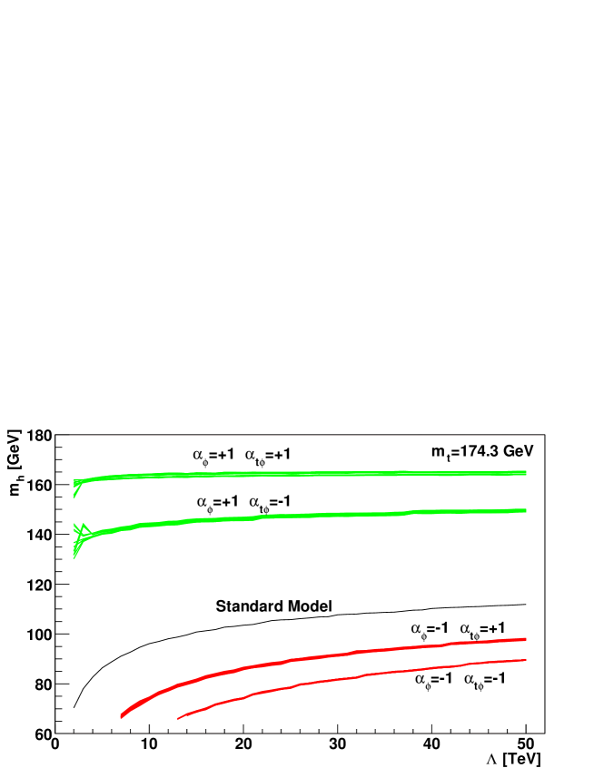
Figure 1: Lower bounds on the Higgs boson mass (all S’s conditions satisfied), the black curve represents the SM limit, the upper (green) curves are for $\alpha_{\phi}>0$, and the lower (red) ones for $\alpha_{\phi}<0$. For each color the higher branches correspond to $\alpha_{t\phi}<0$ while lower for $\alpha_{t\phi}>0$.

Due to its appearance in the tree-level potential (3), $\alpha_{\phi}$ has a strong impact on the vacuum stability bound. For $\alpha_{\phi}(\Lambda)>0$ the corresponding term decreases the value of $V_{\rm eff}$ at $\bar{\varphi}\sim\Lambda$ and a larger value of $\lambda$ is required to stabilize the minimum at $v_{0}$ (thereby insuring condition S2 is satisfied). In this case we then obtain that the vacuum stability constraints are satisfied for values of $m_{h}$ larger than those obtained in the pure SM (for the same choice of $\Lambda$).

When $\alpha_{\phi}(\Lambda)<0$ the effect of the corresponding term in (3) tends to stabilize the minimum at $v_{0}$, but it also shifts it away from the tree-level SM value. Therefore in this case $m_{h}$ is not limited by the stability of $v_{0}$ but by the requirement that its value is near the electroweak scale (condition S1).

We present our stability results in Fig. 1 where we show the 64 curves corresponding to all possible signs of $\alpha_{i}(\Lambda)$ and the SM curve. The black middle curve describes the SM limit, while the non-standard bounds consist of 4 tight groups of 16 curves each: the two upper (green) curves provide the limit for $\alpha_{\phi}(\Lambda)=+1$ while the lower (red) ones for $\alpha_{\phi}(\Lambda)=-1$. The graphs show that $\alpha_{t\phi}>0$ tends to destabilize the electroweak vacuum, and that the limits obtained for fixed $\alpha_{\phi}(\Lambda)$ and $\alpha_{t\phi}(\Lambda)$ are almost independent of the signs of the other $\alpha_{i}(\Lambda)$ (their influence is illustrated by the width of the curves).

In spite of the complicated nature of the analysis performed here, it is worth to trace the way in which $\alpha_{t\phi}$ could influence the lower limit on the Higgs-boson mass. The key point is the fact that ${\cal O}_{t\phi}$ modify the relation (25) between the top-quark mass and its Yukawa coupling. Expressing the Yukawa coupling $f$ through $m_{t}$ one obtains the following form of the fermionic contribution, $T$, to the effective potential (IV):

$$T=\left(\sqrt{2}\frac{m_{t}}{v_{0}}\right)^{2}\bar{\varphi}^{2}\left[1+\sqrt{2}\alpha_{t\phi}\frac{v_{0}}{m_{t}}\frac{\bar{\varphi}^{2}-v_{0}^{2}}{\Lambda^{2}}+{\cal O}\left(\alpha_{t\phi}\frac{v_{0}^{2}}{\Lambda^{2}}\right)\right]\,.$$ (27)

Since the instability (where the effective potential is bending down) takes place for $\bar{\varphi}\gg v_{0}$ therefore effectively we obtain substantial enhancement or suppression (depending on the sign of $\alpha_{t\phi}$) factor of top-quark contribution. Another mechanism of enhancing the contribution from ${\cal O}_{t\phi}$ is the very large numerical factor in front of $\alpha_{t\phi}$ in the evolution equation of $\alpha_{\phi}$. Because of this a larger $\alpha_{t\phi}$ drives $\alpha_{\phi}$ to larger values thereby again requiring a larger $m_{h}$. Both effects combine leading to the dependence on $\alpha_{t\phi}$ illustrated in Fig.1.

It is worth noticing that $\alpha_{\phi}>0$ whenever the effective operator ${\cal O}_{\phi}$ is generated through the tree-level exchange of a heavy scalar isodoublet in the fundamental high-scale theory. This scenario allows for a Higgs boson mass below the SM stability limit, and if this happens to be the case experimentally, the result would not only indicate the presence of new physics, but would also suggest the type of new physics and provide an upper bound on its scale.

V.2 Triviality bounds and combined limits

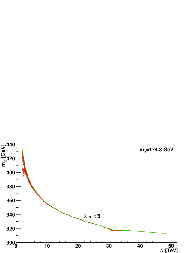
Figure 2: The upper bound on the Higgs boson mass from the standard triviality condition: $\lambda<\pi/2$ (the small-scale structure is due to numerical inaccuracies).

Turning now to the triviality bounds we first note that the restrictions imposed by T1 alone, presented in Fig. 2 remain unchanged in the presence of the effective operators. We include in this plot the SM result together with the 64 curves obtained by taking $\alpha_{i}(\Lambda)=\pm 1$. It is seen that all 65 lines are nearly identical illustrating the fact that the SM upper limit stay approximately unchanged in presence of the effective operators.

To qualitatively understand this lack of sensitivity it is useful to consider the special case where $\alpha_{i\not=\phi}=0$. In this case it follows form (14) that $\alpha_{\phi}(t)$ is a monotonically increasing function of $t$ ; and the numerical coefficients insure a rapid change from $|\alpha_{\phi}(\Lambda)|=1$ to $|\alpha_{\phi}(m_{Z})|\lower 2.15277pt\hbox{$\>\buildrel<\over{\sim}\>$}0.1$. Since $\alpha_{\phi}$ below $\Lambda$ is small, its presence does not significantly affect the evolution of $\lambda$. This is reinforced by the fact that the $\alpha_{i}$-effects are always suppressed by small $\eta\equiv\lambda(v/\Lambda)^{2}$ (a consequence of decoupling). Therefore the corrections to the SM triviality bound from the non-standard physics (embedded in the coefficients $\alpha_{i}$) are negligible . Only for a very small scale $\Lambda\mathrel{\raise 1.29167pt\hbox{$<$\kern-7.5pt\lower 4.30554pt\hbox{$\sim$}}}3\;\hbox{TeV}$ we observe slight deviations from the SM limit.

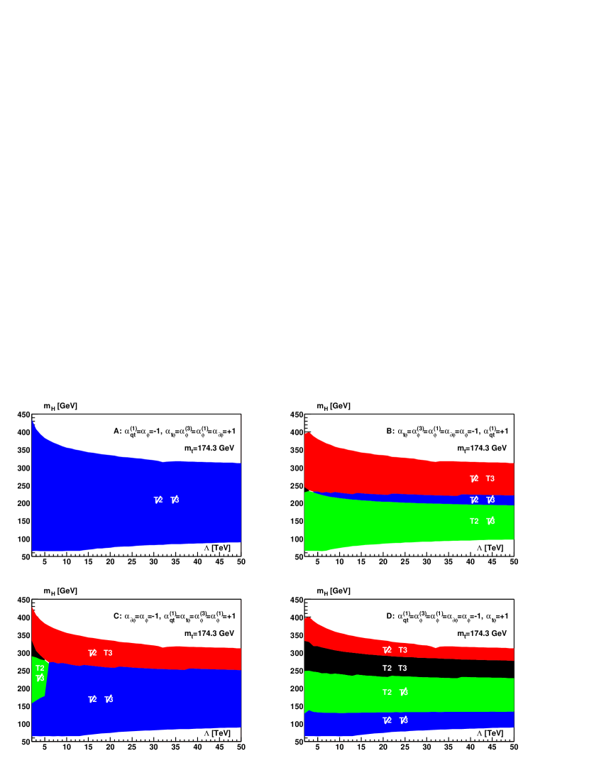
Figure 3: The regions allowed and disallowed by the triviality conditions T2 and T3 for 4 selected combinations of $\alpha_{i}$ specified in the main text as models A, B, C, and D. The black color regions, labeled T2 T3, are such that both conditions are satisfied; red areas, labeled $\not\!\!\hbox{T2}$ T3, represent the regions where T3 is satisfied but T2 is not; green areas, labeled T2 $\not\!\!\hbox{T3}$, represent the regions where T2 is satisfied but T3 is not; and blue areas, labeled $\not\!\!\hbox{T2}$ $\not\!\!\hbox{T3}$, represent the regions where neither T2 nor T3 are satisfied.

The full triviality conditions for this model, however, also requires the imposition of the conditions T2 and T3 and this leads to a rich structure and manifold possibilities. We have picked 4 illustrative cases  with the following parameters:

Case $$-1$$

A

B

C

D

(28)

We have restricted our analysis only to values of $\Lambda$ and $m_{h}$ satisfying all the stability conditions and the triviality condition T1 as presented on Figs. 1 and Fig. 2 respectively. The combined plots (containing both the lower and the upper bounds) corresponding to the models defined above are presented in Fig. 3 where we specify the additional regions excluded by conditions T2 and T3.

The violation of condition T2 is always due to $\alpha_{\phi}$ or $\alpha_{t\phi}$. For large $\lambda$ (corresponding to large $m_{h}$) T2 is similar but stronger than condition T3b, while the opposite is true for small $\lambda$ (i.e. small $m_{h}$). As a result the $\not\!\!\hbox{T2}\hbox{T3}$ region (red) is always next to the upper edge of the region allowed by the triviality condition ($\lambda=\pi/2)$.

The fact that $\hbox{T2}\not\!\!\hbox{T3}$ region (green) or $\not\!\!\hbox{T2}\not\!\!\hbox{T3}$ region (blue) appears always adjoint to the lower edge (where $\lambda$ is relatively small) is also easy to understand, for in this case T3 is stronger, and therefore easier to violate.

Note that there exist models (e.g. the model A) such that either of the requirements T2 and T3 exclude the whole region between the SM-like upper limit ($\lambda<\pi/2$) and the lower (stability) bound, which is due to large contributions to the $\beta$-functions, the tree-level potential and to the Higgs-boson mass from the effective operators. This illustrates the importance of conditions T2 and T3 that can completely eliminate certain models, and severly limt the allowed values of $\Lambda$ and $m_{h}$ in others. These restrictions cannot be obtained using only the standard triviality conditions T1.

As we have already discussed, for the vacuum stability limits only $\alpha_{\phi}$ and $\alpha_{t\phi}$ were relevant. in contrast, the generalized (caused by T2 and/or T3) triviality limits depend on all the $\alpha_{i}$ since none of them plays a preferred role in the RG equations, which leads to the observed rich texture. Note for instance the difference between plots corresponding to models A and C for which $\alpha_{\phi}$ and $\alpha_{t\phi}$ are identical.

It is also worth emphasizing that condition T3 is equivalent to the requirement that the effective operators generate small changes in the $\beta$-functions, the tree-level potential and the Higgs mass. This however, is not relevant for models where there is no relation between the SM and the effective couplings (this would be similar to the top contributions within the SM that need not be small compared to those generated by the gauge fields or the scalars). For such models the regions in Fig. 3 labeled $\not\!\!\hbox{T3}$ are no longer forbidden. It should also be mentioned that the actual strength of the triviality conditions T1, T2 and T3 is to certain extent arbitrary (e.g we could demand deviations below 20% insted of the 25% we used), and therefore shape of the allowed regions showed in Fig.3 could be slightly modified if other conditions were specified.

VI Summary and Conclusions

We have considered restrictions on the Higgs-boson mass that emerge form requirement of perturbative behavior of coupling constants (the triviality bound) and from the condition of stable electroweak vacuum, taking into account possible non-standard interactions (of a typical scale $\Lambda$) described by effective operators of dimension $\leq\;6$. The allowed regions in the ($\Lambda,m_{h}$) space resulting from the stability and triviality requirements has been determined and discussed in detail, taking into account all the necessary constraints from precision tests of the Standard Model. It was shown that for the scale of new physics in the region $2\;\hbox{TeV}\lower 2.15277pt\hbox{$\>\buildrel<\over{\sim}\>$}\Lambda\lower 2.15277pt\hbox{$\>\buildrel<\over{\sim}\>$}50\;\hbox{TeV}$ the Standard Model triviality upper bound (defined as an upper limit for the quartic coupling constant $\lambda$) remains unchanged, whereas the lower bound from the requirement of vacuum stability could be substantially modified, depending on values of the coefficients of two dim 6 operators: ${\cal O}_{\phi}=\frac{1}{3}|\phi|^{6}$ and ${\cal O}_{t\phi}=|\phi|^{2}\left(\bar{q}\tilde{\phi}t+\hbox{h.c.}\right)$. A natural generalization of the triviality condition leads also to a substantial reduction of the allowed region in the ($\Lambda,m_{h}$) space.

All the above considerations are applicable for the case where the heavy physics is weakly coupled and decoupling, and has a particle content that naturally generates the various operators considered, especially ${\cal O}_{\phi}$ and ${\cal O}_{t\phi}$. However, there are models where these operators are not generated  in which case the stability and triviality bounds relax to those of the SM.

Finally we would like to mention that several discrepancies between the results presented here and those of Grzadkowski:2001vb . This is due to a series of typographical errors in Grzadkowski:2001vb : the signs of the $\alpha_{i}$ in the Lagrangian and effective potential (equations 1,3 and 5 of that reference) should be changed. Then the sign convention for $\alpha_{i}$ used in the present paper is opposite to the one used in Grzadkowski:2001vb ; correspondingly the sign of $\alpha_{\phi}$ induced in a 2-higgs doublet model is positive. In addition the triviality graph presented in Grzadkowski:2001vb refers only to the usual SM condition, labeled T1 above; the claims made in Grzadkowski:2001vb concerning the requirement T2 are incorrect.

ACKNOWLEDGMENTS

This work is supported in part by the State Committee for Scientific Research (Poland) under grant 5 P03B 121 20 and funds provided by the U.S. Department of Energy under grant No. DE-FG03-94ER40837. BG and JP are indebted to U.C. Riverside for the warm hospitality extended to them while this work was being performed.

APPENDIX

The issue of the vacuum stability in presence of non-standard physics has been recently addressed by the authors of Ref. Burgess:2002tj . They conjectured that if the ground state of the underlying theory has flat directions (no quartic interactions for certain field configurations), then the effective theory will be non-polynomial and an expansion in powers of light fields is not justified. However, in the absence of fine tuning there will be no flat directions, and these complications do not arise. This is the situation considered in the present paper where the effective potential is by its construction polynomial in light degrees of freedom.

As an illustration of their statement the authors of  Burgess:2002tj provide an model containing two real scalar fields, $\phi$ and $\Phi$, with the following potential

$$V(\phi,\Phi)=-{1\over 2}m^{2}\phi^{2}+{1\over 8}\lambda\phi^{4}+{1\over 2}M^{2}\Phi^{2}+\xi\phi^{3}\Phi+\kappa\phi^{2}\Phi^{2}\ .$$ (29)

Assuming $M^{2}\gg m^{2}>0$, $V$ will have a minimum at $\phi^{2}\simeq 2m^{2}/\lambda$ and $\Phi\simeq 0$ which will be stable provided

$$\kappa>0\ ,\;\;\;\;{\rm and}\;\;\;\;\lambda\geq 2\frac{\xi^{2}}{\kappa}\,.$$ (30)

On the other hand in the effective theory obtained by integrating out the heavy field $\Phi$ one obtains the following low-energy potential:

$$V(\phi)=-{1\over 2}m^{2}\phi^{2}+{1\over 8}\lambda\phi^{4}-{1\over 2}\xi^{2}{\phi^{6}\over M^{2}+2\kappa\phi^{2}}\,.$$ (31)

The authors of Ref. Burgess:2002tj then claim that expanding in powers of $\phi^{2}/M^{2}$ leads to the result that the potential (31) is unstable for parameters that at the same time satisfy the positivity constraints (30) for the underlying theory (29). Their conclusion is then that stability requirements obtained using the low-energy effective theory are inaccurate and can generate much stronger bounds than those obtained using the full Lagrangian.

In order to investigate the effective Lagrangian derived from (31) we note that the large $M$ expansion is justified provided $\kappa\phi^{2}/M^{2}\ll 1$. Adopting this restriction, one can easily find that the effective theory is stable when

$$\lambda\geq 2\frac{\xi^{2}}{|\kappa|}\,.$$ (32)

We thus reproduce the second stability condition in (30); it is clear, however, that to the lowest order in $\kappa\phi^{2}/M^{2}$ we cannot recover the constraint $\kappa>0$. This is so because (32) is the result of physics at or below the cutoff $\Lambda=M/\sqrt{|\kappa|}$. In contrast, the condition on $\kappa$ results from of some physics (or fine tuning) above the cutoff, and cannot be obtained using the effective theory. It should also be emphasized here that the effective Lagrangian approach presupposes that all terms allowed by the symmetries of the model are present in the original Lagrangian, which is not the case for (29); accordingly, the constraint on $\kappa$ is significantly modified if we allow a term $\propto\Phi^{4}$. Though one cannot draw any general conclusions experimenting with a fine tuned potential such as (29), this example does provide a useful illustration of the implications of the naturality assumption in effective theories.

References

- (1) T. Junk, The LEP Higgs Working Group, at LEP Fest October 10th 2000, http://lephiggs.web.cern.ch/LEPHIGGS/talks/index.html.
- (2) E. Tournefier, The LEP Electroweak Working Group, talk presented at the 36th Rencontres De Moriond On Electroweak Interactions And Unified Theories, 2001, Les Arcs, France, hep-ex/0105091.
- (3) K. G. Wilson, Phys. Rev. B 4, 3184 (1971).
- (4) L. Maiani, G. Parisi and R. Petronzio, Nucl. Phys. B 136, 115 (1978); M. Lindner, Z. Phys. C 31, 295 (1986).
- (5) N. Cabibbo et al., Nucl. Phys. B 158, 295 (1979); for a review see M. Sher, Phys. Rep. 179, 273 (1989) and references therein.
- (6) J. A. Casas et al. Nucl. Phys. B 436, 3 (1995) [Erratum-ibid. B 439, 466 (1995)] [hep-ph/9407389]; M. Quiros, IEM-FT-153-97, hep-ph/9703412.
- (7) B. Grzadkowski and J. Wudka, Phys. Rev. Lett. 88, 041802 (2002), hep-ph/0106233; Acta Phys. Polon. B 32, 3769 (2001), hep-ph/0110151.
- (8) A. Datta, B. L. Young and X. Zhang, Phys. Lett. B 385, 225 (1996), hep-ph/9604312.
- (9) J. A. Casas, V. Di Clemente and M. Quiros, Nucl. Phys. B 581, 61 (2000), hep-ph/0002205.
- (10) C. P. Burgess, V. Di Clemente and J. R. Espinosa, JHEP 0201, 041 (2002), hep-ph/0201160.
- (11) S. Weinberg, hep-th/9702027. H. Georgi, Ann. Rev. Nucl. Part. Sci. 43, 209 (1993).
- (12) T. Appelquist and J. Carazzone, Phys. Rev. D 11, 2856 (1975). J. Collins, F. Wilczek and A. Zee, Phys. Rev. D 18, 242 (1978).
- (13) W. Buchmüeller and D. Wyler, Nucl. Phys. B 268, 621 (1986).
- (14) G. ’t Hooft, Lecture given at Cargese Summer Inst., Cargese, France, Aug 26 - Sep 8, 1979, in C79-08-26.4 PRINT-80-0083 (UTRECHT).
- (15) C. Arzt, M.B. Einhorn and J. Wudka, Nucl. Phys. B 433, 41 (1995), hep-ph/9405214.
- (16) L. Dolan and R. Jackiw, Phys. Rev. D 9, 2904 (1974).
- (17) W. Loinaz and R.S. Willey, Phys. Rev. D 56, 7416 (1997), hep-ph/9702321.
- (18) R. Jackiw, Phys. Rev. D 9, 1686 (1974).
- (19) C. Ford et al., Nucl. Phys. B 395, 17 (1993), hep-lat/9210033.
- (20) G. Sanchez-Colon and J. Wudka, Phys. Lett. B 432, 383 (1998), hep-ph/9805366; R. Barbieri and A. Strumia, Phys. Lett. B 462, 144 (1999), hep-ph/9905281; L. Hall and C. Kolda, Phys. Lett. B 459, 213 (1999), hep-ph/9904236; J.A. Bagger, A.F. Falk and M. Swartz, Phys. Rev. D 84, 1385, (2000), hep-ph/9908327.
- (21) W. F. Hollik, Fortsch. Phys. 38, 165 (1990); W. Hollik, MPI-PH-93-21
- (22) K. I. Aoki, Z. Hioki, M. Konuma, R. Kawabe and T. Muta, Prog. Theor. Phys. Suppl. 73, 1 (1982).
- (23) M. Chanowitz, Phys. Rev. D 63, 076002 (2001), hep-ph/0010310.